Abstract
Ski jump spillways are frequently implemented to dissipate energy from high-speed flows. The general feature of this structure is to transform the spillway flow into a free jet up to a location where the impact of the jet creates a plunge pool, representing an area for potential erosion phenomena. In the present investigation, several tests with different ski jump bucket angles are executed numerically by means of the OpenFOAM® digital library, taking advantage of the Reynolds-averaged Navier–Stokes equations (RANS) approach. The results are compared to those obtained experimentally by other authors as related to the jet length and shape, obtaining physical insights into the jet characteristics. Particular attention is given to the maximum pressure head at the tailwater. Simple equations are proposed to predict the maximum dynamic pressure head acting on the tailwater, as dependent upon the Froude number, and the maximum pressure head on the bucket. Results of this study provide useful suggestions for the design of ski jump spillways in dam construction.
1. Introduction
In the field of dam construction, ski jump spillways have been studied for several decades, through the application of simple techniques in earlier investigations. In Ref. [1,2,3], one can obtain a summary of recommended characteristic parameters for the realization of ski jumps (see also [4] for a critical review of formulas for the prediction of scour depth beneath jets from flip buckets).
In this field, some experimental studies have been published. For example, Ref. [5] describes a hydraulic study on a 2-D sectional model at a scale of 1:55 for the design of a two-tier spillway and energy dissipater arrangement. In Ref. [6], a test program on a hydraulic model was conducted aiming to explore how flaring piers and slit bucket structures perform the process of energy dissipation in order to mitigate the erosive effects of effluent jets from spillways. Results indicate that a correlation exists between the deflection angle and the downstream scour hole. In Ref. [7], a new type of streamwise-lateral spillway is suggested against the conventional spillway design methodology. In this approach, a leak-floor flip bucket is presented so that the central portion of the flow is lifted into the atmosphere and then deflected transversally. The optimum free jet flow diffusion was observed at a range of inclination floor angles of 30 to 45°. In Ref. [8], laboratory experiments were performed utilizing a ski jump type energy dissipator in flows with different sediment concentrations. Experimental results were analyzed to study the hydraulic properties of energy dissipation in terms of flow discharge, jet characteristics, and hydrodynamic pressure. The results indicate that the effect of sediment concentration is constant in comparison with the fresh water. The authors of Ref. [9] reported the results of experiments of high-velocity air–water flows on two stepped spillways to explore the scale effects relating to air–water properties: findings emphasized that any notation of scale effects must be considered accurately in terms of a specific set of air–water flow characteristics. In Ref. [10], a study on pressure and aeration in stepped-chute flows was conducted. It was suggested that an aerator should be employed at the end of the step surface in order to avoid cavitation. In Ref. [11], a theoretical and experimental study of the flaring gate piers on the surface of a dam was carried out to investigate flow pattern, discharge capacity, and pressure distribution in the channel. Data analysis depicts a good agreement between theoretical and experimental results. In Ref. [12], effects of geometric parameters of the slit-type dissipater (STED) on energy dissipation were analyzed and the authors of that study concluded that, in a slit type energy dissipater, the behavior of the structure is influenced by the contraction angle.
In Ref. [13], a study on aeration of a jet above the spillway using a dimensional analysis is reported, concluding that the similitude of the air entrainment phenomenon is not possible, and an analytical solution of the upper nappe entrainment is proposed.
In Ref. [14,15,16], an extensive and systematic study of ski jumps is provided: the authors executed a number of experiments on a simplified ski jump configuration downstream of a horizontal approaching channel. The study involved systematic variation of the main effective parameters, namely relative bucket curvature, bucket deflection angle, and approaching Froude number.
In the numerical field, Ref. [17] simulated the ski jump flows of the streamwise-lateral discharge spillway, taking advantage of the Reynolds-averaged Navier–Stokes equations (RANS). A comparison between the numerical and experimental results showed that the optimum range of the lateral spillway inclination angle is 30 to 45°. In Ref. [18,19], a numerical procedure was conducted to analyze different aspects of this subject: the hydraulic behavior of ski jumps was investigated by means of the OpenFOAM® digital library and by following formulations of a RANS approach. Results were compared to those obtained experimentally by Ref. [15], depicting good agreement. Particular attention was given to the issues of the falling jet length and to the visualization of the dynamic pressure head distribution in the impact area of the jet.
It is to be noted that the majority of these investigations are actually case studies and may not be adopted to be generalized. Furthermore, the magnitude and location of maximum pressure head acting on the tailwater have not been adequately studied. The numerical model used in this study is calibrated by means of the results of laboratory experiments of other authors ([15,18]). Afterwards, several simulations are executed, with particular attention paid to the maximum value and distribution of pressure heads at critical zones where the jet impacts.
2. Materials and Methods
The Reynolds-averaged Navier–Stokes equations are solved numerically for the simulation of the jet flow cases reported in Table 1, taken from Ref. [15]. The equations are as follows:

Table 1.
Characteristic parameters of numerical simulations.
Herein, is fluid density, the dynamic water viscosity, the mean fluid pressure, are the mean velocity components, are the mean strain-rate tensor:
and represent the Reynolds stress tensor.
Following the Boussinesq approximation [20,21], the eddy viscosity is set as a function of the turbulent kinetic energy and the energy dissipation rate. In order to establish a relation between the Reynolds stress and the mean-flow quantities, the k-omega SST model [22] is utilized as follows (see also [23,24]):
In order to prevent the build-up of turbulence in stagnation regions, the production limiter is embedded in the model. in the above equation denotes a blending function, expressed as
in which and y stands for the distance to the nearest wall.
The turbulent eddy viscosity is , where , S is the second invariant of the deviatoric stress tensor, and represents a second blending function and is computed as
The constants of the above formulations are computed with a blend from; for example, . The closure coefficients of the selected model are , , , , , , . The k-ω SST model generally performs well in complex flow cases (see, e.g., [21,22,25]).
The interFoam solver (embedded in the OpenFoam® C++ libraries) is used to solve numerically the governing Equations (1) and (2), together with the equations of the turbulence model. The solver takes into account the VoF (volume of fluid) [26] phase-fraction interface capturing approach. This technique allows us to locate and track the free surface, providing satisfactory results [27,28,29,30].
To each fluid phase (i.e., air and water), an individual fraction of the volume is associated (see [26]), so that the indicator function is defined as
The two-phase flow is considered a mixed fluid. Therefore, the density and the dynamic viscosity are expressed as
in which subscripts 1 and 2 represent the two fluids [31], and the volume-fraction function is predicted by solving an advection equation:
For the discretization of the governing equations, the finite volumes technique is utilized (FVM, see [31], among others). An unstructured mesh in a co-located arrangement and the PISO method (pressure implicit with split operator [32]) are utilized to couple the pressure and velocity in transient computations. The PISO technique is developed on the basis of a segregated methodology, and the equations are solved sequentially (details can be obtained from [31]). An adaptive time step having an initial value of 1 × 10⁻⁶ s and a mean Courant–Friedrichs–Lewy (CFL) number limit of 0.5 is considered to ensure the stability of the solution procedure.
The laboratory channel used for the numerical simulations has the same characteristics of that described in Ref. [15]: an approach flow channel having a width b = 0.50 m, height of 0.70 m and a total length of 7 m, along with bucket radius R and bucket angle β (Figure 1). With an approaching flow depth h0 and the discharge Q, the bulk flow velocity is calculated as V0 = Q/(bh0). The approaching flow characteristics can be defined in terms of the approaching flow Froude number F0 = V0/(gh0)1/2, and the relative bucket radius h0/R, while the magnitude of the bucket height w = R(1 − cosβ) is related to the free-bucket flows. g represents acceleration due to the gravity. Note that Figure 1 is a definition sketch to show geometric parameters of a ski jump jet. In general, air entrainment occurs in such a phenomenon that is not shown in the simplified Figure 1. However, this paper includes photos of laboratory experiments that illustrate real jet flows.
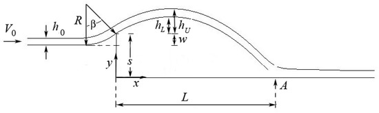
Figure 1.
Definition sketch and geometric parameters of a ski jump flow.
Figure 1 also shows hU and hL that represent the upper and lower levels reached by the jet, respectively. In Figure 1, s−w denote the difference between the elevation of the approaching flow and the tailwater elevation, A is the point where the maximum dynamic pressure head verifies, and L is the length of the jet measured from the origin of the reference system along the x direction.
The imposed boundary conditions at the channel bed (tailwater), the sidewalls and the bucket are no-slip and zero wall-normal velocity. At the inlet section, the flow depth ho and bulk flow velocity V0 as reported in Table 1 were assigned; at the outlet cross-section, the gradient of flow velocity was set to zero in the direction perpendicular to the boundary and the free-surface condition was enforced at the flow free surface. The numerical channel was initially empty and the simulations were run until the jet reached its final configuration (i.e., no variation was observed in jet characteristics).
Concerning the grid resolution, the computational mesh was refined through ascending the grid points in the stream-normal direction (Nx = 335, 340, 345, 350, Ny = 100, Nz = 50), up to the point at which no difference was observed in the characteristics of the maximum dynamic pressure head acting on the bucket centerline compared with the previous configuration. The ultimate configuration of the computational domain consists of a total number of grid points Ntot = 1,750,000 (Nx = 350, Ny = 100, Nz = 50, see Ref. [18], Figure 2). For the numerical simulations, a CPU-based computational system was employed that included 1 worker node with 4 E5-2640 CPUs, 128 GB RAM at 1899 MHz, and 1 TB disk space. The simulations were conducted taking advantage of the public domain OpenMPI implementation of the standard message passing interface (MPI). Moreover, the “simple geometric decomposition” technique was utilized. In this method, the domain is divided into segments by direction.
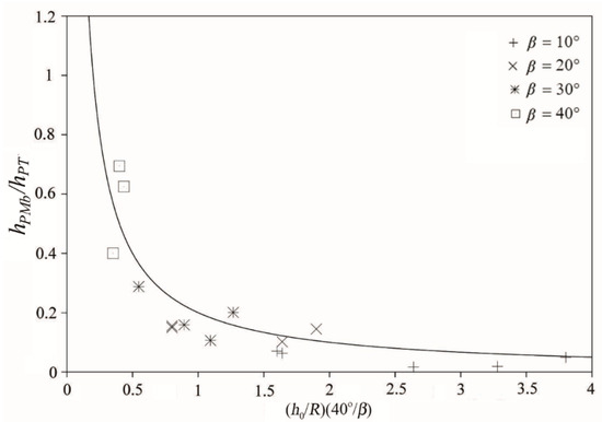
Figure 2.
Behavior of the dynamic pressure head on bucket centerline: (―) ratio between the maximum calculated and the theoretical pressure heads from Equation (12) versus the ratio between the maximum calculated and the theoretical pressure head from the present study (symbols).
3. Results and Discussion
Table 1 reports the characteristic parameters of numerical simulations of ski jump flow in the present study. The simulated cases are compared to those obtained from the laboratory tests [15], in terms of pressure magnitudes on the bucket and behavior of jet trajectories.
Figure 2 provides a comparison between the computed nondimensional maximum dynamic pressure heads on the bucket centerline at different bucket deflection angles β and the calculated results from the empirical Equation (12) for ([15]):
whereas for , the theoretical value is obtained from Equation (13):
in which is the approach bend number, i.e., the square root of relative bucket radius multiplied by the approach Froude number. hPMb and hPT are maximum dynamic pressure head on the bucket centerline and theoretical dynamic pressure head, respectively. This figure shows how smaller bucket angles produce smaller maximum pressure heads. Figure 3 shows a comparison between the computed nondimensional dynamic pressure heads along the bucket centerline hP for different magnitudes of β and the computed results from Equation (14) [15].
where XPM=x/xPM stands for relative location of the maximum pressure head and P = hPT/hPMb is the relative pressure head [15].
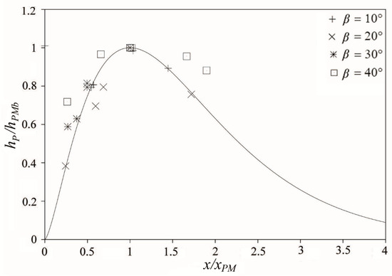
Figure 3.
Local pressure head distribution along the bucket centerline: (―) calculated values with Equation (5) in [15] versus the computed values from the present study (symbols).
This figure implies that satisfactory agreements are achieved for the selected bucket angles except for β = 40°, for which the predicted values are slightly above the trend line calculated by the mentioned empirical equation. From Figure 3, it is also evident that the computed results agree well with the peak of the trend line.
Figure 4 illustrates the computed values of nondimensional upper (a) and lower (b) jet trajectories for different Froude numbers against the calculated values with Equation (15) [15]:
where , and αj is the jet takeoff angle. It is clear that the computed results are properly in accordance with the obtained results from the empirical formula. In Figure 4, and denote takeoff angles of the lower and the upper jet trajectories with respect to a horizontal plane. Accordingly, and represent the upper and lower jet trajectories.
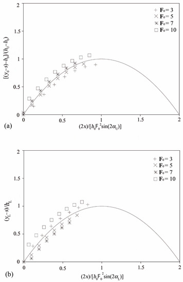
Figure 4.
(a) Upper jet trajectory: (―) calculated by Equation (7) in [18] versus the computed values in the present study (symbols); (b) lower jet trajectory: (―) calculated with Equation (7) in [15] versus the computed values in the present study (symbols).
Previous studies [15,18,19] indicated that the takeoff angles of the lower and upper boundaries vary with the relative bucket curvature and the bucket deflection angle and that the takeoff angles are almost identical to the deflection angles only for the case of small relative curvature. Overall, the comparison between the data of previous studies and those resulting from the present study is satisfactory, showing that the numerical scheme of this investigation is able to solve the considered flow cases accurately.
In Figure 5 and Figure 6, some visual comparisons of jets from ski jumps (R = 0.10 m, β = 40°, h0 = 0.05 m) at two significantly different Froude numbers (F0 = 5 and 10, respectively, Tests 27 and 29 in Table 1) are shown (side view). In these figures, a picture of the experimental jets in Ref. [15] is compared with those obtained in the present work in terms of velocity fields. The reddish colors represent the highest values of the fluid velocities, while the bluish colors are attributable to the lowest values. High values of the fluid velocity can be observed in the jet core and the largest values are located immediately upstream to the impact zone of the falling jet. A recirculation zone can be observed between the end of the bucket and the point at which the jet impinges the tailwater channel. Both the upper and lower jet trajectories follow a parabolic path. The fluid velocity increases along the jet trajectory and the lower free surface properly detaches from the bucket.
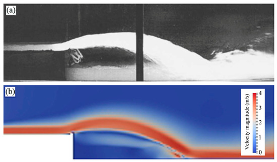
Figure 5.
Visual comparison between the ski jump jets for R = 0.10 m, β = 40°, h0 = 0.05 m, F0 = 5 (test no. 27 in Table 1: (a) physical experiment [15] (reproduced with permission from ASCE); (b) numerical results of the present study (note: the darkest red color represents velocity magnitudes of 4 m/s and larger).
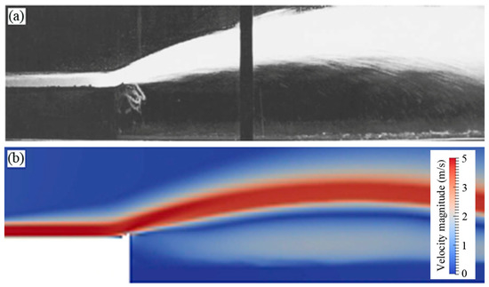
Figure 6.
Visual comparison between the ski jump jets for R = 0.10 m, β = 40°, h0 = 0.05 m, F0 = 10 (test no. 29 in Table 1: (a) physical experiment [15] (reproduced with permission from ASCE); (b) numerical results of the present study (note: the darkest red color represents velocity magnitudes of 5 m/s and larger).
Dynamic pressure-head surface for F0 = 5 and 10 and its projection onto the x-z plane in the impact zone the jet (i.e., on the tailwater channel) is illustrated in Figure 7. In this figure, the pressure head hP is normalized with the maximum pressure head value acting on tailwater region hPMt. The reddish colors in Figure 7a represent the largest head magnitudes, while the bluish colors mirror the smallest values. In fact, the reddish area within the quasi-rectangular sub-region (i.e., the zone of the largest heads) is related to the impact region of the jet onto the tailwater channel. Figure 7b exhibits the distribution of nondimensional dynamic pressure head along the z-axis, where the maximum magnitude of the pressure head occurs. The distribution is not fully symmetric and depicts only one value of the absolute maximum pressure head (points with label B).
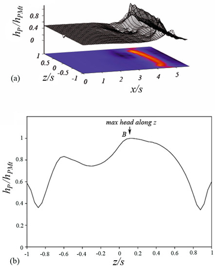
Figure 7.
Behavior of the dynamic pressure head on the tailwater channel for F0 = 5 and R = 0.10 m, β = 40°, h0 = 0.05 m, test no. 27 in Table 1: (a) three-dimensional depiction of the nondimensional dynamic pressure head; (b) distribution of nondimensional dynamic pressure head along the z-axis.
Figure 8a shows the three-dimensional depiction of the nondimensional dynamic pressure-head for test no. 29 with a much larger Froude number. This figure also shows that the maximum dynamic pressure head occurs within the tailwater channel. Figure 8b shows the nondimensional dynamic pressure head distribution along the z-axis, where the maximum magnitudes of the pressure head are located. In contrast to test no. 27, with a smaller Froude number, the distribution is almost symmetric and exhibits three maxima, noting that the pressure at point B on the right portion of the figure is slightly larger than the other two peaks.
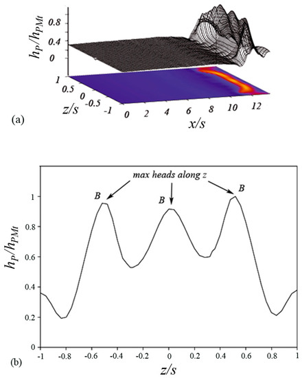
Figure 8.
Behavior of the dynamic pressure head on the tailwater channel for F0 = 10 and R = 0.10 m, β = 40°, h0 = 0.05 m, test no. 27 in Table 1: (a) three-dimensional depiction of nondimensional dynamic pressure head; (b) distribution of nondimensional dynamic pressure head along the z-axis.
Figure 7 and Figure 8 imply that the dynamic pressure head of the F0 = 5 case is distributed in a larger area with respect to what happens at F0 = 10, where the maximum dynamic pressure heads exhibit as three clearly distinguishable peaks.
Figure 9 presents correlating lines between F0 values and nondimensional maximum dynamic pressure heads acting on the tailwater zone of the ski jump flow with R = 0.10 m. Note that the maximum pressure head value acting on tailwater region hPMt is normalized with the approaching flow depth h0. From Figure 9, the following formulas are derived:
valid for R = 0.10 m, β = 10°, 3 ≤ F0 ≤ 10 and 1.27 ≤ hPMt/h0 ≤ 24.48, with a coefficient of determination r2 = 0.916;
valid for R = 0.10 m, β = 20°, 3 ≤ F0 ≤ 10 and 5.455 ≤ hPMt/h0 ≤ 25.35, with a coefficient of determination r2 = 0.971;
valid for R = 0.10 m, β = 30°, 3 ≤ F0 ≤ 10 and 3.71 ≤ hPMt/h0 ≤ 24.68, with a coefficient of determination r2 = 0.981; and
valid for R = 0.10 m, β = 40°, 3 ≤ F0 ≤ 10 and 4.71 ≤ hPMt/h0 ≤ 14.31, with a coefficient of determination r2 = 0.976.
F0 = 0.275(hPMt/h0) + 3.384
F0 = 0.326(hPMt/h0) + 1.854
F0 = 0.339(hPMt/h0) + 1.746
F0 = 0.760(hPMt/h0) − 1.023
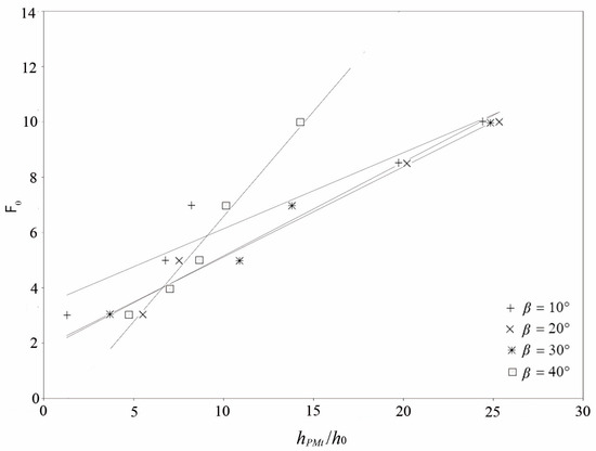
Figure 9.
Correlations between the approach Froude numbers F0 and the maxima dynamic pressure heads hPMt/h0 acting on tailwater zone for the simulations with R = 0.10 m.
The resulting large r2 values confirm that simple linear regression properly correlates the selected parameters. One may observe that the hPMt/h0 magnitude varies in the range of 1.27 to 25.35 and increases with F0. Figure 9 also clarifies that the correlation lines for β = 10°, 20°, and 30° (Equations (16)–(18)) have a similar behavior in a very wide range of hPMt/h0, while as for the remaining case, i.e., β = 40° (Equation (19)), a considerable large variation of F0 occurs in a small range of hPMt/h0. This finding may suggest that for bucket angles β < 30° and for a certain value of F0, the bucket angle itself may induce a greater dynamic pressure head.
Figure 10 presents correlating lines between nondimensional maximum dynamic pressure heads on the bucket and nondimensional maximum dynamic pressure heads acting on tailwater region for the ski jump flow with R = 0.10 m. The maximum pressure head acting on the bucket hPMb is normalized with the approaching flow depth h0. From the chart of Figure 10, the following equations are derived:
valid for R = 0.10 m, β = 10°, 0.42 ≤ hPMb/h0 ≤ 2.6 and 1.27 ≤ hPMt/h0 ≤ 24.48, with a coefficient of determination r2 = 0.93;
valid for R = 0.10 m, β = 20°, 1.24 ≤ hPMb/h0 ≤ 5.98 and 5.45 ≤ hPMt/h0 ≤ 25.35, with a coefficient of determination r2 = 0.99;
valid for R = 0.10 m, β = 30°, 1.72 ≤ hPMb/h0 ≤ 11.79 and 3.71 ≤ hPMt/h0 ≤ 24.68, with a coefficient of determination r2 = 0.93;
valid for R = 0.10 m, β = 40°, 2 ≤ hPMb/h0 ≤ 13.58 and 4.71 ≤ hPMt/h0 ≤ 14.31, with a coefficient of determination r2 = 0.96.
hPMb/h0 = 0.104(hPMt/h0) − 0.066
hPMb/h0 = 0.224(hPMt/h0) + 0.164
hPMb/h0 = 0.503(hPMt/h0) − 1.33
hPMb/h0 = 1.256(hPMt/h0) − 4.985
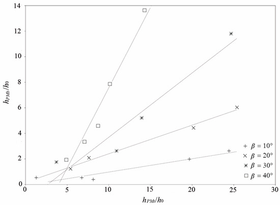
Figure 10.
Chart of correlation lines between values of the nondimensional maximum dynamic pressure head acting on tailwater hPMt/h0 and nondimensional maximum dynamic pressure head acting on bucket hPMb/h0 for the simulations with R = 0.10 m.
The obtained charts from the application of three-dimensional RANS equations (Figure 9 and Figure 10) may be considered a useful tool to estimate the maximum dynamic pressure heads acting on tailwaters and buckets of the ski jump spillways. It should be noted that, by definition, the RANS equations are averaged. In fact, this kind of turbulence model does not predict pressure fluctuations and maximum instantaneous pressure magnitudes. Even though the use of RANS may provide adequate information about the pressure head for practical purposes and engineering applications, a more accurate estimation of maximum pressure heads may be obtained by means of the models that predict velocity and pressure fluctuations (e.g., use of large-eddy simulation approach).
4. Conclusions
A numerical study on the hydraulics of ski jump flow has been executed. The issue of the dynamic pressure head acting on the tailwater and the bucket of a ski jump jet has been particularly investigated in detail. Both the maximum value and the distribution of dynamic pressure head acting on the zone affected by the falling jet have been analyzed. This study may also provide useful information for researchers who are trying to find solutions to protect this area from erosion. One may conclude that, in order to avoid the complexities of performing laboratory experiments, numerical simulations could be considered as alternative and effective tools.
This study clarifies that approaching flow Froude number and the maximum dynamic pressure head acting on tailwater are correlated. This is a useful technique for prediction of the latter quantity from the approaching flow Froude number and the selected bucket angle β. The second chart indicates that there is a correlation between the maximum dynamic pressure head acting on tailwater and the maximum dynamic pressure head acting on the bucket. Therefore, engineers are able to predict maximum dynamic pressure head acting on critical locations of a ski jump flow (i.e., tailwater regions and buckets) from the approaching flow Froude number and the selected bucket angle.
Author Contributions
Conceptualization, A.L. and G.A.; methodology, A.L., G.A. and A.T.; software, A.L.; validation, A.T., G.A. and A.T.; data curation, A.L. and G.A.; writing—original draft preparation, A.L., G.A. and A.L.; supervision, A.L. All authors have read and agreed to the published version of the manuscript.
Funding
This research received no external funding.
Conflicts of Interest
The authors declare no conflict of interest.
References
- Rajan, B.H.; Rao, K.N. Design of trajectory buckets. Water Energy Int. 1980, 37, 63–76. [Google Scholar]
- Rao, K.N.S. Design of Energy Dissipators for Large Capacity Spillways. In Proceedings of the International Congress on Large Dams, Rio de Janeiro, Brazil, 3–7 May 1982; Volume 1, pp. 311–328. [Google Scholar]
- Mason, P.J. Practical guidelines for the design of flip buckets and plunge pools. Int. Water Power Dam Constr. 1993, 45, 40–45. [Google Scholar]
- Mason, P.J.; Arumugam, K. Free jet scour below dams and flip buckets. J. Hydraul. Eng. 1985, 111, 220–235. [Google Scholar] [CrossRef]
- Bhate, R.R.; More, K.T.; Bhajantri, M.R.; Bhosekar, V.V. Hydraulic model studies for optimizing the design of two tier spillway—A case study. ISH J. Hydraul. Eng. 2019, 25, 28–37. [Google Scholar]
- De Lara, R.; Ota, J.J.; Fabiani, A.L.T. Reduction of the erosive effects of effluent jets from spillways by contractions in the flow. RBRH 2018, 23, e11. [Google Scholar] [CrossRef]
- Deng, J.; Wei, W.; Tian, Z.; Zhang, F. Ski Jump Hydraulics of Leak-Floor Flip Bucket. In Proceedings of the 7th International Symposium on Hydraulic Structures, Aachen, Germany, 15–18 May 2018. [Google Scholar]
- Gou, W.; Li, H.; Du, Y.; Yin, H.; Liu, F.; Lian, J. Effect of Sediment Concentration on Hydraulic Characteristics of Energy Dissipation in a Falling Turbulent Jet. Appl. Sci. 2018, 8, 1672. [Google Scholar] [CrossRef]
- Felder, S.; Chanson, H. Scale effects in microscopic air-water flow properties in high-velocity free-surface flows. Exp. Therm. Fluid Sci. 2017, 83, 19–36. [Google Scholar] [CrossRef]
- Xu, W.; Luo, S.; Zheng, Q.; Luo, J. Experimental study on pressure and aeration characteristics in stepped chute flows. Sci. China Technol. Sci. 2015, 58, 720–726. [Google Scholar] [CrossRef]
- Li, N.-W.; Liu, C.; Deng, J.; Zhang, X.-Z. Theoretical and Experimental Studies of the Flaring Gate Pier on the Surface Spillway in a High-Arch Dam. J. Hydrodyn. 2012, 24, 496–505. [Google Scholar] [CrossRef]
- Wu, J.-H.; Ma, F.; Yao, L. Hydraulic Characteristics of Slit-Type Energy Dissipaters. J. Hydrodyn. 2012, 24, 883–887. [Google Scholar] [CrossRef]
- Chanson, H. Aeration of a free jet above a spillway. J. Hydraul. Res. 1991, 29, 655–667. [Google Scholar] [CrossRef]
- Juon, R.; Hager, W.H. Flip Bucket without and with Deflectors. J. Hydraul. Eng. 2000, 126, 837–845. [Google Scholar] [CrossRef]
- Heller, V.; Hager, W.H.; Minor, H.-E. Ski Jump Hydraulics. J. Hydraul. Eng. 2005, 131, 347–355. [Google Scholar] [CrossRef]
- Hager, W.H.; Boes, R.M. Hydraulic structures: A positive outlook into the future. J. Hydraul. Res. 2014, 52, 299–310. [Google Scholar] [CrossRef]
- Deng, J.; Wei, W.; Tian, Z.; Zhang, F. Design of A Streamwise-Lateral Ski-Jump Flow Discharge Spillway. Water 2018, 10, 1585. [Google Scholar] [CrossRef]
- Lauria, A.; Alfonsi, G. Numerical Investigation of Ski Jump Hydraulics. J. Hydraul. Eng. 2020, 146, 04020012. [Google Scholar] [CrossRef]
- Lauria, A.; Alfonsi, G. Numerical Simulation of Ski-Jump Hydraulic Behavior. In Numerical Computations: Theory and Algorithms, Proceedings of the Third International Conference, NUMTA 2019, Crotone, Italy, 15–21 June, 2019; Revised Selected Papers, Part II; Springer International Publishing: Rende, Italy, 2019; Volume 11974, pp. 422–429. ISBN 978-3-030-40616-5. [Google Scholar] [CrossRef]
- Wilcox, D.C. Turbulence Modeling for CFD; DCW Industries: La Cañada, CA, USA, 1998. [Google Scholar]
- D’Ippolito, A.; Lauria, A.; Alfonsi, G.; Calomino, F. Investigation of flow resistance exerted by rigid emergent vegetation in open channel. Acta Geophys. 2019, 67, 971–986. [Google Scholar] [CrossRef]
- Menter, F.R.; Kuntz, M.; Langtry, R. Ten Years of Industrial Experience with the SST Turbulence Model. In Proceedings of the 4th International Symposium on Turbulence, Heat and Mass Transfer, Antalya, Turkey, 12–17 October 2003; pp. 625–632. [Google Scholar]
- Menter, F.R. Zonal Two-Equation k-ω Turbulence Model for Aerodynamic Flows. In Proceedings of the 23rd Fluid Dynamics, Plasma Dynamics and Lasers Conference, Orlando, FL, USA, 6–9 July 1993; pp. 2906–2916. [Google Scholar]
- Menter, F.R. Two-equation eddy-viscosity turbulence models for engineering applications. AIAA J. 1994, 32, 1598–1605. [Google Scholar] [CrossRef]
- Calomino, F.; Alfonsi, G.; Gaudio, R.; D’Ippolito, A.; Lauria, A.; Tafarojnoruz, A.; Artese, S. Experimental and Numerical Study of Free-Surface Flows in a Corrugated Pipe. Water 2018, 10, 638. [Google Scholar] [CrossRef]
- Hirt, C.; Nichols, B. Volume of fluid (VOF) method for the dynamics of free boundaries. J. Comput. Phys. 1981, 39, 201–225. [Google Scholar] [CrossRef]
- Rusche, H. Computational Fluid Dynamics of Dispersed Two-Phase Flows at High Phase Fractions. Ph.D. Thesis, University of London, London, UK, 2002. [Google Scholar]
- Alfonsi, G.; Ferraro, D.; Lauria, A.; Gaudio, R. Large-eddy simulation of turbulent natural-bed flow. Phys. Fluids 2019, 31, 085105. [Google Scholar] [CrossRef]
- Alfonsi, G.; Lauria, A.; Primavera, L. Structures of a Viscous-Wave Flow around a Large-Diameter Circular Cylinder. J. Flow Vis. Image Process. 2012, 19, 323–354. [Google Scholar] [CrossRef]
- Alfonsi, G.; Lauria, A.; Primavera, L. The Field of Flow Structures Generated by a Wave of Viscous Fluid Around Vertical Circular Cylinder Piercing the Free Surface. Procedia Eng. 2015, 116, 103–110. [Google Scholar] [CrossRef][Green Version]
- Jasak, H. Error Analysis and Estimation for the Finite Volume Method with Applications to Fluid Flows. Ph.D. Thesis, Imperial College, London, UK, 1996. [Google Scholar]
- Issa, R.I. Solution of the implicitly discretized fluid flow equations by operator-splitting. J. Comput. Phys. 1986, 62, 40–65. [Google Scholar]


© 2020 by the authors. Licensee MDPI, Basel, Switzerland. This article is an open access article distributed under the terms and conditions of the Creative Commons Attribution (CC BY) license (http://creativecommons.org/licenses/by/4.0/).