CFD Julia: A Learning Module Structuring an Introductory Course on Computational Fluid Dynamics

Abstract

CFD Julia is a programming module developed for senior undergraduate or graduate-level coursework which teaches the foundations of computational fluid dynamics (CFD). The module comprises several programs written in general-purpose programming language Julia designed for high-performance numerical analysis and computational science. The paper explains various concepts related to spatial and temporal discretization, explicit and implicit numerical schemes, multi-step numerical schemes, higher-order shock-capturing numerical methods, and iterative solvers in CFD. These concepts are illustrated using the linear convection equation, the inviscid Burgers equation, and the two-dimensional Poisson equation. The paper covers finite difference implementation for equations in both conservative and non-conservative form. The paper also includes the development of one-dimensional solver for Euler equations and demonstrate it for the Sod shock tube problem. We show the application of finite difference schemes for developing two-dimensional incompressible Navier-Stokes solvers with different boundary conditions applied to the lid-driven cavity and vortex-merger problems. At the end of this paper, we develop hybrid Arakawa-spectral solver and pseudo-spectral solver for two-dimensional incompressible Navier-Stokes equations. Additionally, we compare the computational performance of these minimalist fashion Navier-Stokes solvers written in Julia and Python.

1. Introduction

Coursework in computational fluid dynamics (CFD) usually starts with an introduction to discretization techniques of partial differential equations (PDEs), stability analysis of numerical methods, the order of convergence, iterative methods for elliptic equations, shock-capturing methods for compressible flows, and development of incompressible flow solver. A lot of emphases is put on the theory of discretization, stability analysis, and different formulations of governing equations for compressible and incompressible flows. Students can gain a better understanding of CFD subject with actual hands-on programming of numerical solutions to mathematical models that present different fluid behavior. To develop a flow solver from scratch is a fairly complex task. Therefore, almost all developmental CFD courses begin with one-dimensional problems to explain theory and fundamentals and then build on to complicated problems like compressible or incompressible flow solvers.

CFD Julia is a programming module that contains several codes for problems ranging from one-dimensional heat equation to two-dimensional Navier-Stokes incompressible flow solver. Some of these problems can be included as part of programming assignments or coursework projects. We include different types of problems, different techniques to solve the same problem and try to introduce CFD using a practical approach. There are a couple of programming modules available online related to CFD. CFD Python learning module is a set of Jupyter notebooks that tries to teach CFD in twelve steps [1]. This module also contains bonus modules for numerical stability analysis, and advanced programming in Python using Numpy [2]. It starts with an introduction to Python and ends with the development of incompressible flow solver for lid-driven cavity problem and channel flow. There is an online module available for a course on numerical methods covering finite difference methods [3]. The material for this coursework was created using IPython notebooks. HyperPython is a set of IPython notebooks created to teach hyperbolic conservation laws [4]. HyperPython module covers high-resolution methods for compressible flows and also teaches how one can use the PyClaw package to solve compressible flow problems. PyClaw is a hyperbolic PDE solver in 1D, 2D, and 3D and it has several features like parallel implementation and choice of higher-order accurate numerical methods [5].

In this work, we use Julia programming language [6] as a tool to develop codes for fundamental CFD problems. Julia is a new programming language which first appeared in the year 2012 and it has gained popularity in the scientific community in recent years. There is a number of programming languages that are already available such as Fortran [7], Python [8], C/C++ [9], Matlab [10], etc. Many of the state of the art CFD codes are written in Fortran and C/C++ because of their high-performance characteristics. Python and Matlab programming languages have simple syntax and students usually use these languages with ease in their coursework. Since the developer’s language is different from the user’s language, there will always be a hindrance to developing numerical codes. Many times a user has to resort to developer’s language like C/C++ for getting the fast performance or have to use other packages to exchange information between codes written in different languages. Julia tries to solve this two-language problem. Julia language was designed to have the syntax that is easy to understand and will also have fast computational performance. Julia shows that one can have machine performance without sacrificing human convenience. Julia tries to achieve the Fortran performance through the automatic translation of formulas into efficient executable code. It allows the user to write clear, high-level, generic code that resembles mathematical formulas. Julia’s ability to combine high-performance with productivity makes it the perfect choice for scientists working in different scientific domains.

In this paper, we use finite difference discretization for different types of PDEs encountered in CFD. For all problems, we provide the main script in Julia so that reader will get familiar with the Julia syntax. We start with the heat equation as the prototype of parabolic PDE. We present an explicit forward in time numerical scheme and implicit Crank-Nicolson numerical scheme for the heat equation. We also cover the multistage Runge-Kutta numerical approach to show how we can get higher temporal accuracy by taking multiple steps between two time intervals. We derive an implicit compact Pade scheme for the heat equation. This will give the reader an understanding of high-resolution numerical methods which are widely used in the direct numerical simulation (DNS) and large eddy simulation (LES). All fundamental concepts related to finite difference numerical methods are covered in Section 2 with the help of heat equation. This will lay the foundation of CFD and will familiarize the reader with basic concepts of discretization methods which will be used further for more complex problems.

We then present the hyperbolic equation in Section 3 using the inviscid Burgers equation. Hyperbolic equations allow having a discontinuous solution. Therefore, higher-order numerical methods have been developed that can capture discontinuities such as shocks. We present weighted essentially non-oscillatory (WENO) formulation for finite difference schemes and show their capability to capture shock using one-dimensional case. We show the mathematical formulation of WENO schemes, their implementation in Julia for two different boundary conditions. We use Dirichlet boundary condition and periodic boundary condition for the inviscid Burgers equation. This will help the reader to understand how to treat different boundary conditions in CFD problems. We also present a compact reconstruction of WENO scheme which has better accuracy and resolution characteristic than the WENO scheme with the price of solving a tridigonal system. Furthermore, we present discretization of the inviscid Burgers equation in its conservative form using different finite difference grid arrangement. This type of formulation is more applicable to finite volume method. We present a method of flux splitting and constructing flux at the interface using a Riemann solver approach in Section 4. We use a Riemann solver approach to solve the one-dimensional Euler equation and is presented in Section 5. The Euler equation solver is demonstrated for Sod shock tube problem using three different Riemann solvers: Rusanov scheme, Roe scheme, and Harten-Lax-van Leer Contact (HLLC) scheme.

We present different methods for solving elliptic partial differential equations using the Poisson equation as an example in Section 6. The Poisson equation is a boundary value problem and is encountered in solution to incompressible flow problems. We show different methods for solving the Poisson equation and their implementation in Julia. We demonstrate direct solver using fast Fourier transform (FFT) for periodic boundary condition problem and fast sine transform (FST) for Dirichlet boundary condition. We also present different iterative methods for solving elliptic equations. We demonstrate the implementation of Gauss-Seidel iterative method and the conjugate gradient method in Julia. The readers will learn the application of both stationary and non-stationary iterative methods. We also show the implementation of a V-cycle multigrid solver to accelerate the convergence of iterative methods.

We show solution to incompressible Navier-Stokes equation with vorticity-streamfunction formulation in Section 7. This is one of the simplest formulations to Navier-Stokes equation as there is no coupling between the velocity and pressure. This allows us to use collocated grid and not a staggered grid for the Navier-Stokes equation. We present a periodic boundary condition case using the vortex-merger problem. The Dirichlet boundary condition case is demonstrated using the lid-driven cavity problem. We use the direct solver to solve the elliptic equation giving the relation between vorticity and streamfunction. However, any of the iterative methods can also be used. We use second-order Arakawa numerical scheme which has better energy conservation properties for the discretization of the Jacobian term. The reader will get familiar with different types of numerical methods apart from standard finite difference schemes with these examples. This type of formulation can also be used for different types of problems such as two-dimensional decaying turbulence, and Taylor green vortex problem. Additionally, we present hybrid Arakawa-spectral solver for two-dimensional incompresible Navier-Stokes equations in Section 8. The flow solver is hybridized using explicit and implicit scheme for time integration. Also, the Navier-Stokes equations are solved in its Fourier space with the nonlinear term computed in physical space using Arakawa finite difference scheme and converted to Fourier space. Section 9 details the implementation fully pseudo-spectral solver for two-dimensional Navier-Stokes equations. We show two approaches to reduce aliasing error: 3/2 padding and 2/3 padding rules. We also show the comparison between CPU time for codes written in Julia and Python for solving the Navier-Stokes equations.

CFD Julia module covers several topics pertinent to both compressible and incompressible flows. This module provides different finite difference codes that will help students learn not just the fundamentals of CFD but also the implementation of numerical methods to solve CFD problems. Using these examples, students can go about developing their solvers for more challenging problems for their coursework or research. We make all these codes available on Github and are accessible to everyone (https://github.com/surajp92/CFD_Julia). Table 1 outlines all codes available in the CFD Julia module with their Github index. Table 1 presents a summary of topics covered and numerical schemes employed for problems included in the CFD Julia module. We write results for all problems into a text file and then use separate plotting scripts to plot results. We provide installation instruction for Julia and required packages, and plotting scripts in Appendix A and Appendix B.

Table 1. Summary of different problems included in the CFD Julia module and the description of topics covered in these selected problems. Source codes are accessible to everyone at https://github.com/surajp92/CFD_Julia.

Github Index	Description
01	1D heat equation: Forward time central space (FTCS) scheme
02	1D heat equation: Third-order Runge-Kutta (RK3) scheme
03	1D heat equation: Crank-Nicolson (CN) scheme
04	1D heat equation: Implicit compact Pade (ICP) scheme
05	1D inviscid Burgers equation: WENO-5 with Dirichlet and periodic boundary condition
06	1D inviscid Burgers equation: CRWENO-5 with Dirichlet and periodic boundary conditions
07	1D inviscid Burgers equation: Flux-splitting approach with WENO-5
08	1D inviscid Burgers equation: Riemann solver approach with WENO-5 using Rusanov solver
09	1D Euler equations: Roe solver, WENO-5, RK3 for time integration
10	1D Euler equations: HLLC solver, WENO-5, RK3 for time integration
11	1D Euler equations: Rusanov solver, WENO-5, RK3 for time integration
12	2D Poisson equation: Finite difference fast Fourier transform (FFT) based direct solver
13	2D Poisson equation: Spectral fast Fourier transform (FFT) based direct solver
14	2D Poisson equation: Fast sine transform (FST) based direct solver for Dirichlet boundary
15	2D Poisson equation: Gauss-Seidel iterative method
16	2D Poisson equation: Conjugate gradient iterative method
17	2D Poisson equation: V-cycle multigrid iterative method
18	2D incompressible Navier-Stokes equations (cavity flow): Arakawa, FST, RK3 schemes
19 *	2D incompressible Navier-Stokes equations (vortex merging): Arakawa, FFT, RK3 schemes
20	2D incompressible Navier-Stokes equations (vortex merging): Hybrid RK3/CN approach
21 *	2D incompressible Navier-Stokes equations (vortex merging): Hybrid pseudo-spectral 3/2 padding approach
22	2D incompressible Navier-Stokes equations (vortex merging): Hybrid pseudo-spectral 2/3 padding approach

* The codes for these problems are provided in Python in addition to Julia language.

2. Heat Equation

We start with the one-dimensional heat equation, which is one of the simplest and most basic models to introduce the concept of finite difference methods. The one-dimensional heat equation is given as

$$\frac{\partial u}{\partial t}=\alpha \frac{{\partial }^{2}u}{\partial x^2},$$

(1)

where u is the field variable, t is the time variable, and $\alpha$ is the diffusivity of the medium. The heat equation describes the evolution of the field variable over time in a medium.

There are different methods to discretize the heat equation, such as, finite volume method [11], finite difference method [12], finite element method [13], spectral methods [14], etc. In this paper, we will study the finite difference method to discretize all partial differential equations (PDEs). The finite difference method is comparatively simpler and is easy to understand in the initial stage of learning CFD. The finite difference method converts the linear or nonlinear PDEs into a set of linear or nonlinear ordinary differential equations (ODEs). These ODEs can be solved using matrix algebra techniques.

Before starting with the derivation of finite difference scheme for the heat equation, we define a grid of points in the $(t,x)$ plane. Let $\Delta x$ and $\Delta t$ be the grid spacing in space and time direction, respectively. Therefore, $(t_n,x_i)=(n\Delta t,i\Delta x)$ for arbitrary integers n and i as shown in Figure 1. We use the notation $u_i^{(n)}$ for $u(t_n,x_i)$.

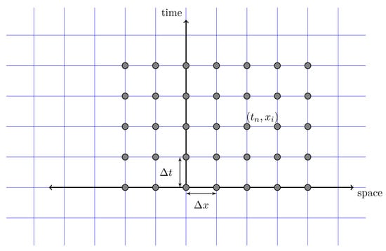
Figure 1. Finite difference grid for one-dimensional problems.

The finite difference method uses Taylor series expansion to derive the discrete approximation for PDEs. Taylor series gives the series expansion of a function f about a point. Taylor series expansion for a function f about the point $x_0$ is given by:

$$f(x_0+\Delta x)=f(x_0)+\frac{\Delta x}{1!}\frac{\partial f(x_0)}{\partial x}+\frac{{\Delta x}^2}{2!}\frac{{\partial }^{2}f(x_0)}{\partial x^2}+\cdots +\frac{{\Delta x}^n}{n!}\frac{{\partial }^{n}f(x_0)}{\partial x^n}+{\mathcal{T}}_n(x),$$

(2)

where $n!$ denotes the factorial of n, and ${\mathcal{T}}_n$ is a truncation term, giving the difference between the Taylor series expansion of degree n and the original function. The difference between the exact solution to the original differential equation and finite difference approximation is termed as the discretization or truncation error. The leading term in the discretization error determines the accuracy of the finite difference scheme. The finite difference scheme for any PDE must have two properties: consistency and stability to ensure the convergence. We would like to suggest a textbook “Finite difference schemes and partial differential equations” [15] which explains numerical behavior of finite difference scheme in detail. In this paper, we focus on the application of the finite difference method to study problems encountered in CFD.

2.1. Forward Time Central Space (FTCS) Scheme

We derive the forward time central space (FTCS) numerical scheme for approximating the heat equation. Using the Taylor series expansion in time for the discrete field $u_i^{(n)}$, we get

$$\begin{array}{cc}\hfill u_i^{(n+1)}& =u_i^{(n)}+\frac{\partial u_i^{(n)}}{\partial t}\Delta t+\mathcal{O}(\Delta t^2),\hfill \end{array}$$

(3)

$$\begin{array}{cc}\hfill \frac{\partial u_i^{(n)}}{\partial t}& =\frac{u_i^{(n+1)}-u_i^{(n)}}{\Delta t}+\mathcal{O}(\Delta t).\hfill \end{array}$$

(4)

Equation (4) is the first-order accurate expression for the time derivative term in the heat equation. To obtain the finite difference formula for second-derivative term in the heat equation, we write the Taylor series expansion for $u_{i+1}^{(n)}$ and $u_{i-1}^{(n)}$ about $u_i^{(n)}$

$$\begin{array}{cc}\hfill u_{i+1}^{(n)}& =u_i^{(n)}+\frac{\partial u_i^{(n)}}{\partial x}\Delta x+\frac{{\partial }^2{u}_i^{(n)}}{\partial x^2}\frac{{\Delta x}^2}{2!}+\frac{{\partial }^3{u}_i^{(n)}}{\partial x^2}\frac{\Delta x^3}{3!}+\mathcal{O}(\Delta x^4),\hfill \end{array}$$

(5)

$$\begin{array}{cc}\hfill u_{i-1}^{(n)}& =u_i^{(n)}-\frac{\partial u_i^{(n)}}{\partial x}\Delta x+\frac{{\partial }^2{u}_i^{(n)}}{\partial x^2}\frac{{\Delta x}^2}{2!}-\frac{{\partial }^3{u}_i^{(n)}}{\partial x^2}\frac{\Delta x^3}{3!}+\mathcal{O}(\Delta x^4).\hfill \end{array}$$

(6)

Adding Equations (5) and (6) and dividing by $\Delta x^2$, we get the second-order accurate formula for second-derivative term in heat equation

$$\frac{{\partial }^2{u}_i^{(n)}}{\partial x^2}=\frac{u_{i+1}^{(n)}-2u_i^{(n)}+u_{i-1}^{(n)}}{{\Delta x}^2}+\mathcal{O}({\Delta x}^2).$$

(7)

Substituting Equations (4) and (7) in Equation (1), we get the FTCS numerical scheme for the heat equation as given below

$$\begin{array}{c}\hfill \frac{u_i^{(n+1)}-u_i^{(n)}}{\Delta t}=\alpha \frac{u_{i+1}^{(n)}-2u_i^{(n)}+u_{i-1}^{(n)}}{{\Delta x}^2},\end{array}$$

(8)

and we can re-write Equation (8) as an explicit update formula

$$\begin{array}{c}\hfill u_i^{(n+1)}=u_i^{(n)}+\frac{\alpha \Delta t}{{\Delta x}^2}\left(u_{i+1}^{(n)}-2u_i^{(n)}+u_{i-1}^{(n)}\right).\end{array}$$

(9)

We denote the above formula as $\mathcal{O}(\Delta t,{\Delta x}^2)$ formula meaning that the leading term of the discretization error is first-order accurate in time and second-order accurate in space. We can obtain the higher-order formula using the larger stencil to get better approximations. If the initial solution to the heat equation is given, then we can proceed in time to get the solution at future times using Equation (9). We can observe from Equation (9), that the solution at the next time step depends only on the solution at previous time steps. These numerical schemes are called an explicit numerical scheme. They are simple to code. However, explicit numerical schemes are restricted by some stability criteria. The stability criteria restricts the maximum step size we can use in spatial and temporal direction and hence explicit numerical schemes are computationally expensive.

We will now demonstrate how one can go about finding the solution at the final time step given an initial condition. We use the computational domain $x\in [-1,1]$ and $\alpha =1/{\pi }^2$. The initial condition for our problem is $u(t=0,x)=-\sin (\pi x)$. We use $\Delta x=0.025$ and $\Delta t=0.0025$ for spatial and temporal discretization. First, we initialize the array u and assign each element of the array using an initial condition. The solution after one time step is calculated using Equation (9) and we will store the solution in first column of matrix un[k,i] (variable in Julia) with the shape $(N_x+1)\times (N_t+1)$, where $N_x$ is the number of divisions of the domain and $N_t$ is the number of time steps between initial and final time. There is no need to store the solution at every time step, and we can just store the solution at intermediate time steps in a temporary array. Here, we store the solution at every time step to see how the field u evolves. The main script of the code which computes and stores the numerical solution at every time step is given in Listing 1.

We compare the solution at final time $t=1$ using the analytical solution to the one-dimensional heat equation. The analytical solution for Equation (1) is given by

$$u(t,x)=-e^{-t}\sin (\pi x).$$

(10)

We also compute the absolute error at $t=1$ using the below formula

$$ϵ(x_i)=|{u_i}^{exact}-u_i^{numerical}|.$$

(11)

Listing 1. Implementation of FTCS numerical scheme for heat equation in Julia.

The comparison of the exact and numerical solution using the FTCS scheme and absolute error plot are shown in Figure 2. We see that we get a very good agreement between the exact and numerical solution due to very small grid size in both space and temporal direction. If we use a larger grid size, then we will see deprecation in accuracy.

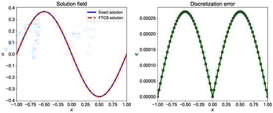
Figure 2. Comparison of exact solution and numerical solution computed using FTCS numerical scheme. The numerical solution is computed using $\Delta t=0.0025$ and $\Delta x=0.025$.

2.2. Runge-Kutta Numerical Scheme

We saw in Section 2.1 that the accuracy of the numerical scheme depends upon the number of terms included from the Taylor series expansion. One of the ways to increase accuracy is to include more terms. The additional term involves partial derivative of $f(x,t)$ which provides additional information on f at $t=t_n$. For the time stepping, we only have information about the data at one or more time steps and the analytical form of f is not known between two time steps. Runge-Kutta methods tries to improve the accuracy of temporal term by evaluating f at intermediate points between $t_n$ and $t_{n+1}$. The additional steps lead to an increase in computational time, but the temporal accuracy is increased.

We use a third-order accurate Runge-Kutta scheme [16] for the discretization of the temporal term in the heat equation. We use the same second-order central difference scheme for the spatial term. The truncation error of this numerical approximation of heat equation is $\mathcal{O}({\Delta t}^3,{\Delta x}^2)$. We move from time step $t_n$ to $t_{n+1}$ using three steps. The time integration of the heat equation using third-order Runge-Kutta scheme is given below:

$$\begin{array}{cc}\hfill u_i^{(1)}& =u_i^{(n)}+\frac{\alpha \Delta t}{{\Delta x}^2}\left(u_{i+1}^{(n)}-2u_i^{(n)}+u_{i-1}^{(n)}\right),\hfill \end{array}$$

(12)

$$\begin{array}{cc}\hfill u_i^{(2)}& =\frac{3}{4}{u}_i^{(n)}+\frac{1}{4}{u}_i^{(1)}+\frac{\alpha \Delta t}{4{\Delta x}^2}\left(u_{i+1}^{(n)}-2u_i^{(n)}+u_{i-1}^{(n)}\right),\hfill \end{array}$$

(13)

$$\begin{array}{cc}\hfill u_i^{(n+1)}& =\frac{1}{3}{u}_i^{(n)}+\frac{2}{3}{u}_i^{(2)}+\frac{2\alpha \Delta t}{3{\Delta x}^2}\left(u_{i+1}^{(n)}-2u_i^{(n)}+u_{i-1}^{(n)}\right).\hfill \end{array}$$

(14)

We can also construct the higher-order Runge-Kutta numerical scheme using more intermediate steps. The implementation of the third-order Runge-Kutta numerical scheme in Julia is given in Listing 2. The comparison of the exact and numerical solutions using the Runge-Kutta scheme and absolute error plot is shown in Figure 3. The discretization error is less for Runge-Kutta numerical scheme compared to the FTCS numerical scheme due to a higher-order approximation of temporal term.

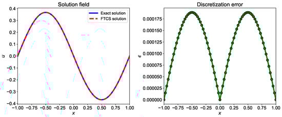
Figure 3. Comparison of exact solution and numerical solution computed using third-order Runge-Kutta numerical scheme. The numerical solution is computed using $\Delta t=0.0025$ and $\Delta x=0.025$.

Listing 2. Implementation of third-order Runge-Kutta numerical scheme for heat equation in Julia.

2.3. Crank-Nicolson Scheme

The Crank-Nicolson scheme is a second-order accurate in time numerical scheme. The Crank-Nicolson scheme is derived by combining forward in time method at $(n)$ and the backward in time method at $(n+1)$. Similar to Equation (3), we can write the Taylor series in time for the discrete field $u_i^{(n+1)}$ as

$$\begin{array}{cc}\hfill u_i^{(n)}& =u_i^{(n+1)}-\frac{\partial u_i^{(n+1)}}{\partial t}\Delta t+\mathcal{O}(\Delta t^2),\hfill \end{array}$$

(15)

$$\begin{array}{cc}\hfill \frac{\partial u_i^{(n+1)}}{\partial t}& =\frac{u_i^{(n+1)}-u_i^{(n)}}{\Delta t}+\mathcal{O}(\Delta t).\hfill \end{array}$$

(16)

The second-derivative term in heat equation at ${(n+1)}^{th}$ time step can be approximated using the second-order central difference scheme similar to the way we derived in Section 2.1

$$\frac{{\partial }^2{u}_i^{(n+1)}}{\partial x^2}=\frac{u_{i+1}^{(n+1)}-2u_i^{(n+1)}+u_{i-1}^{(n+1)}}{{\Delta x}^2}+\mathcal{O}({\Delta x}^2).$$

(17)

Substituting finite difference approximation derived in Equations (16) and (17) in the heat equation, we get

$$\frac{u_i^{(n+1)}-u_i^{(n)}}{\Delta t}=\alpha \frac{u_{i+1}^{(n+1)}-2u_i^{(n+1)}+u_{i-1}^{(n+1)}}{{\Delta x}^2}.$$

(18)

If we add Equations (8) and (18), the leading term in discretization error cancels each other due to their opposite sign and same magnitude. Hence, we get the second-order accurate in time numerical scheme. The Crank-Nicolson scheme is $\mathcal{O}({\Delta t}^2,{\Delta x}^2)$ numerical scheme. The Crank-Nicolson scheme is given as

$$\frac{u_i^{(n+1)}-u_i^{(n)}}{\Delta t}=\frac{\alpha }{2}\left[\frac{u_{i+1}^{(n)}-2u_i^{(n)}+u_{i-1}^{(n)}}{{\Delta x}^2}+\frac{u_{i+1}^{(n+1)}-2u_i^{(n+1)}+u_{i-1}^{(n+1)}}{{\Delta x}^2}\right].$$

(19)

We observe from the above equation that the solution at ${(n+1)}^{th}$ time step depends on the solution at previous time step ${(n)}^{th}$ and the solution at ${(n+1)}^{th}$ time step. Such numerical schemes are called implicit numerical schemes. For implicit numerical schemes, the system of algebraic equations has to be solved by inverting the matrix. For one-dimensional problems, the tridiagonal matrix is formed and can be solved efficiently using the Thomas algorithm, which gives a fast $\mathcal{O}(N)$ direct solution as opposed to the usual $\mathcal{O}(N^3)$ for a full matrix, where N is the size of the square tridiagonal matrix. The main advantage of an implicit numerical scheme is that they are unconditionally stable. This allows the use of larger time step and grid size without affecting the convergence of the numerical scheme. An illustration of a tridiagonal system is given in Equation (20). The Thomas algorithm [17] used for solving the tridiagonal matrix is outlined in Algorithm 1.

$$\underset{\phantom{(}A}{\left[\begin{array}{ccccc}{b}_1& c_1& 0& \cdots & 0\\ a_2& b_2& c_2& \cdots & 0\\ ⋮& ⋮& & \ddots & ⋮\\ 0& \cdots & a_{N-1}& b_{N-1}& c_{N-1}\\ 0& 0& \cdots & a_N& b_N\end{array}\right]}\underset{\phantom{(}\mathit{u}}{\left[\begin{array}{c}{u}_1\\ u_2\\ ⋮\\ u_{N-1}\\ u_N\end{array}\right]}=\underset{\phantom{(}\mathit{d}}{\left[\begin{array}{c}{d}_1\\ d_2\\ ⋮\\ d_{N-1}\\ d_N\end{array}\right]}.$$

(20)

Algorithm 1 Thomas algorithm
1: Given $\mathit{a},\mathit{b},\mathit{c},\mathit{d}$	▹ $A\mathit{u}=\mathit{d}$
2: Allocate $\mathit{q}$	▹ Storage of superdiagonal array
3: $u_1=d_1/b_1$
4: for $i=2$ to N do	▹ Forward elimination
5:  $q_i=c_{i-1}/b_{i-1}$
6:  $b_i=b_i-q_i{a}_i$
7:  $u_i=(d_i-a_i{u}_{i-1})/b_i$
8: end for
9: for $i=N-1$ to 1 do	▹ Backward substitution
10:  $u_i=(u_i-q_{i+1}{u}_{i+1})$
11:end for

The implementation of the Crank-Nicolson numerical scheme for the heat equation is presented in Listing 3 and Thomas algorithm in Listing 4. The comparison of exact and numerical solution computed using the Crank-Nicolson scheme, and absolute error plot are displayed in Figure 4. The absolute error between the exact and numerical solution is less for the Crank-Nicolson scheme than the FTCS numerical scheme due to smaller truncation error.

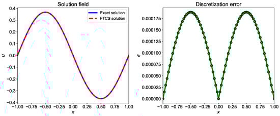
Figure 4. Comparison of exact solution and numerical solution computed using Crank-Nicolson numerical scheme. The numerical solution is computed using $\Delta t=0.0025$ and $\Delta x=0.025$.

Listing 3. Implementation of Crank-Nicolson numerical scheme for heat equation in Julia.

Listing 4. Implementation of Thomas algorithm to solve tridiagonal system of equations in Julia.

2.4. Implicit Compact Pade (ICP) Scheme

We usually use the order of accuracy as an indicator of the ability of finite difference schemes to approximate the exact solution as it tells us how the discretization error will reduce with mesh refinement. Another way of measuring the order of accuracy is the modified wavenumber approach. In this approach, we see how much the modified wave number is different from the true wave number. The solution of a nonlinear partial differential equation usually contains several frequencies and the modified wavenumber approach provides a way to assess how well the different components of the solution are represented. The modified wavenumber varies for every finite difference scheme and can be found using Fourier analysis of the differencing scheme [12].

Compact finite difference schemes have very good resolution characteristics and can be used for capturing high-frequency waves [18]. In compact formulation, we express the derivative of a function as a linear combination of values of function defined on a set of nodes. The compact method tries to mimic global dependence and hence has good resolution characteristics. Lele [18] investigated the behavior of compact finite difference schemes for approximating a first and second derivative. The fourth-order accurate approximation to the second derivative is given by

$$\frac{1}{12}\frac{{\partial }^{2}u}{\partial x^2}{|}_{i-1}+\frac{10}{12}\frac{{\partial }^{2}u}{\partial x^2}{|}_i+\frac{1}{12}\frac{{\partial }^{2}u}{\partial x^2}{|}_{i+1}=\frac{u_{i-1}-2u_i+u_{i+1}}{{\Delta x}^2}.$$

(21)

Taking the linear combination of heat equation and using the same coefficients as the above equation, we get

$$\frac{1}{12}\frac{\partial u}{\partial t}{|}_{i-1}+\frac{10}{12}\frac{\partial u}{\partial t}{|}_i+\frac{1}{12}\frac{\partial u}{\partial t}{|}_{i+1}=\frac{u_{i-1}-2u_i+u_{i+1}}{{\Delta x}^2}.$$

(22)

We then use Crank-Nicolson numerical scheme for time discretization and we arrive to below equation

$$\frac{u_{i-1}^{(n+1)}-u_{i-1}^{(n)}}{12\Delta t}+10\frac{u_i^{(n+1)}-u_i^{(n)}}{12\Delta t}+\frac{u_{i+1}^{(n+1)}-u_{i+1}^{(n)}}{12\Delta t}=\frac{u_{i-1}^{(n+1)}-2u_i^{(n+1)}+u_{i+1}^{(n+1)}+u_{i-1}^{(n)}-2u_i^{(n)}+u_{i+1}^{(n)}}{{2\Delta x}^2}.$$

(23)

Simplifying above equation, we get the implicit compact Pade (ICP) scheme for heat equation

$$a_i{u}_{i-1}^{(n+1)}+b_i{u}_i^{(n+1)}+c_i{u}_{i+1}^{(n+1)}=r_i^{(n)},$$

(24)

where

$$\begin{array}{cc}\hfill a_i& =\frac{12}{{\Delta x}^2}-\frac{2}{\alpha \Delta t},\hfill \end{array}$$

(25)

$$\begin{array}{cc}\hfill b_i& =\frac{-24}{{\Delta x}^2}-\frac{20}{\alpha \Delta t},\hfill \end{array}$$

(26)

$$\begin{array}{cc}\hfill c_i& =\frac{12}{{\Delta x}^2}-\frac{2}{\alpha \Delta t},\hfill \end{array}$$

(27)

$$\begin{array}{cc}\hfill r_i& =\frac{-2}{\alpha \Delta t}\left(u_{i-1}^{(n+1)}-2u_i^{(n+1)}+u_{i+1}^{(n+1)}\right)-\frac{12}{{\Delta x}^2}\left(u_{i-1}^{(n)}-2u_i^{(n)}+u_{i+1}^{(n)}\right).\hfill \end{array}$$

(28)

The ICP numerical scheme forms the tridiagonal matrix which can be solved using the Thomas algorithm to get the solution. The implementation of the ICP numerical scheme in Julia is given in Listing 5. Figure 5 shows the comparison of the exact and numerical solution and discretization error for ICP scheme. The ICP scheme is $\mathcal{O}({\Delta t}^2,{\Delta x}^4)$ accurate scheme and hence, the discretization error is very small.

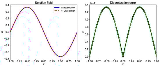
Figure 5. Comparison of exact solution and numerical solution computed using implicit compact Pade numerical scheme. The numerical solution is computed using $\Delta t=0.0025$ and $\Delta x=0.025$.

Listing 5. Implementation of implicit compact scheme Pade numerical scheme for heat equation in Julia.

3. Inviscid Burgers Equation: Non-Conservative Form

In this section, we discuss the solution of the inviscid Burgers equation which is a nonlinear hyperbolic partial differential equation. The hyperbolic equations admit discontinuities, and the numerical schemes used for solving hyperbolic PDEs need to be higher-order accurate for smooth solutions, and non-oscillatory for discontinuous solutions [19]. The inviscid Burgers equation is given below

$$\frac{\partial u}{\partial t}+u\frac{\partial u}{\partial x}=0.$$

(29)

First we use FTCS numerical scheme for discretization of the inviscid Burgers equation as follow

$$\frac{u_i^{(n+1)}-u_i^{(n)}}{\Delta t}+u_i^{(n)}\frac{u_{i+1}^{(n)}-u_{i-1}^{(n)}}{2\Delta x}=0.$$

(30)

We use the shock generated by a sine wave to demonstrate the capability of FTCS numerical scheme to compute the numerical solution. The initial condition is $u_0=\sin (2\pi x)$. We integrate the solution from time $t=0$ to $t=0.25$ with $\Delta t=0.0001$ and divide the computational domain into 200 grids. The numerical solution computed by FTCS at 10 equally spaced time steps between initial and final time is shown in Figure 6. It can be observed that the FTCS scheme does not capture the shock formed at $x=0.5$ and produce oscillations in the solution. It can be demonstrated that FTCS scheme is numerically unstable for advection equations.

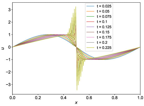
Figure 6. Evolution of shock with time for the initial condition $u_0=\sin (2\pi x)$ using FTCS scheme.

There are several ways in which the discontinuity in the solution (e.g., shock) can be handled. There are classical shock-capturing methods like MacCormack method, Lax-Wanderoff method, and Beam-Warming method as well as flux limiting methods [20,21]. We can also use higher-order central difference schemes with artificial dissipation [22]. Low pass filtering might also help to diminish the growth of the instability modes [23]. There is also a class of modern shock capturing methods called as high-resolution schemes. These high-resolution schemes are generally upwind biased and take the direction of the flow into account. Here, in particular, we discuss higher-order weighted essentially non-oscillatory (WENO) schemes [24] that are used widely as shock-capturing numerical methods. We also use compact reconstruction weighted essentially non-oscillatory (CRWENO) schemes [25] which have lower truncation error compared to WENO schemes.

3.1. WENO-5 Scheme

We refer readers to a text by Shu [26] for a comprehensive overview of the development of WENO schemes, their mathematical formulation, and the application of WENO schemes for convection dominated problems. We will use WENO-5 scheme for one-dimensional inviscid Burgers equation with the shock developed by a sine wave. We will discuss how one can go about applying WENO reconstruction for finite difference schemes. The finite difference approximation to the inviscid Burgers equation in non-conserved form can be written as

$$\begin{array}{cc}\hfill \frac{\partial u_i}{\partial t}+u_i\frac{u_{i+\frac{1}{2}}^L-u_{i-\frac{1}{2}}^L}{\Delta x},& \mathrm{if}{u}_i>0\hfill \end{array}$$

(31)

$$\begin{array}{cc}\hfill \frac{\partial u_i}{\partial t}+u_i\frac{u_{i+\frac{1}{2}}^R-u_{i-\frac{1}{2}}^R}{\Delta x},& \mathrm{otherwise},\hfill \end{array}$$

(32)

which can be combined into a more compact upwind/downwind notation as follows

$$\frac{\partial u_i}{\partial t}+u_i^{+}\frac{u_{i+\frac{1}{2}}^L-u_{i-\frac{1}{2}}^L}{\Delta x}+u_i^{-}\frac{u_{i+\frac{1}{2}}^R-u_{i-\frac{1}{2}}^R}{\Delta x}=0,$$

(33)

where we define $u_i^{+}=\max (u_i,0)$ and $u_i^{-}=\min (u_i,0)$. the reconstruction of $u_{i+\frac{1}{2}}^L$ uses a biased stencil with one more point to the left, and that for $u_{i+\frac{1}{2}}^R$ uses a biased stencil with one more point to the right. The stencil used for reconstruction of left and right side state (i.e., $u_{i+1/2}^L$ and $u_{i+1/2}^R$) is shown in Figure 7. The WENO-5 reconstruction for left and right side reconstructed values is given as [24]

$$\begin{array}{c}\hfill u_{i+\frac{1}{2}}^L=w_0^L\left(\frac{1}{3}{u}_{i-2}-\frac{7}{6}{u}_{i-1}+\frac{11}{6}{u}_i\right)+w_1^L\left(-\frac{1}{6}{u}_{i-1}+\frac{5}{6}{u}_i+\frac{1}{3}{u}_{i+1}\right)+w_2^L\left(\frac{1}{3}{u}_i+\frac{5}{6}{u}_{i+1}-\frac{1}{6}{u}_{i+2}\right),\end{array}$$

(34)

$$\begin{array}{c}\hfill u_{i-\frac{1}{2}}^R=w_0^R\left(-\frac{1}{6}{u}_{i-2}+\frac{5}{6}{u}_{i-1}+\frac{1}{3}{u}_i\right)+w_1^R\left(\frac{1}{3}{u}_{i-1}+\frac{5}{6}{u}_i-\frac{1}{6}{u}_{i+1}\right)+w_2^R\left(\frac{11}{6}{u}_i-\frac{7}{6}{u}_{i+1}+\frac{1}{3}{u}_{i+2}\right),\end{array}$$

(35)

where nonlinear weights are defined as

$$w_k^L=\frac{{\alpha }_k}{{\alpha }_0+{\alpha }_1+{\alpha }_2},{\alpha }_k=\frac{d_k^L}{{({\beta }_k+ϵ)}^2},k=0,1,2$$

(36)

$$w_k^R=\frac{{\alpha }_k}{{\alpha }_0+{\alpha }_1+{\alpha }_2},{\alpha }_k=\frac{d_k^R}{{({\beta }_k+ϵ)}^2},k=0,1,2$$

(37)

in which the smoothness indicators are defined as

$$\begin{array}{cc}\hfill {\beta }_0& =\frac{13}{12}{(u_{i-2}-2u_{i-1}+u_i)}^2+\frac{1}{4}{(u_{i-2}-4u_{i-1}+3u_i)}^2,\hfill \end{array}$$

(38)

$$\begin{array}{cc}\hfill {\beta }_1& =\frac{13}{12}{(u_{i-1}-2u_i+u_{i+1})}^2+\frac{1}{4}{(u_{i-1}-u_{i+1})}^2,\hfill \end{array}$$

(39)

$$\begin{array}{cc}\hfill {\beta }_2& =\frac{13}{12}{(u_i-2u_{i+1}+u_{i+2})}^2+\frac{1}{4}{(3u_i-4u_{i+1}+3u_{i+2})}^2.\hfill \end{array}$$

(40)

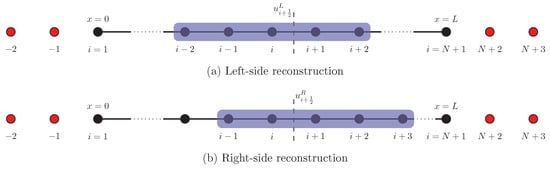
Figure 7. Finite difference grid for one-dimensional problems where the the solution is stored at the interface of the cells. The first and last points lie on the left and right boundary of the domain. The stencil required for reconstruction of left and right side state is highlighted with blue rectangle. Ghost points are shown by red color.

We use $d_0^L=1/10$, $d_1^L=3/5$, and $d_2^L=3/10$ in Equation (36) to compute nonlinear weights for calculation of left side state using Equation (34) and $d_0^R=3/10$, $d_1^R=3/5$, and $d_2^R=1/10$ in Equation (37) to compute nonlinear weights for calculation of right side state using Equation (35). We set $ϵ=1\times {10}^{-6}$ to avoid division by zero. To avoid repetition, we provide only the implementation of Julia function to compute the left side state in Listing 6. The right side state is computed in a similar way with coefficients for $d_k^R$ in Equation (37).

We perform the time integration using third-order Runge-Kutta numerical scheme as discussed in Section 2.2 and its implementation is similar to Listing 2. The right hand side term of the inviscid Burgers equation is computed using the point value $u_i$ and the derivative term is evaluated using the left and right side states at the interface. Based on the direction of flow i.e., the sign of $u_i$, we either use left side state or right side state to compute the derivative. The implementation of right hand side state calculation in Julia for the inviscid Burgers equation is given in Listing 7.

Listing 6. Implementation of left side state calculation function in Julia.

Listing 7. Implementation of right hand side calculation for the inviscid Burgers equation in Julia.

We demonstrate two types of boundary conditions for the inviscid Burgers equation. The first one is the Dirichlet boundary condition. For Dirichlet boundary condition, we use $u(x=0)=0$ and $u(x=1)=0$. For computing numerical state at the interface, we need the information of five neighboring grid points (see Figure 7). When we compute the left side state at $i+\frac{1}{2}$ interface, we use three points on left side (i.e., $u_{i-2},u_{i-1},u_i$) and two points on right side (i.e., $u_{i+1},u_{i+2}$). Therefore, we use two ghost points on the left side of the domain and one ghost point on right side of the domain for computing left side state (i.e., $u^L$ at $x=3/2$ and $x=N-1/2$ respectively). Similarly, we use one ghost points on the left side of the domain and two ghost point on right side of the domain for computing right side state (i.e., $u^R$ at $x=3/2$ and $x=N-1/2$ respectively). We use linear interpolation to compute the value of discrete field u at ghost points. The computation of u at ghost points is given below

$$\begin{array}{cc}\hfill u_{-2}& =3u_1-2u_2,u_{-1}=2u_1-u_2,\hfill \end{array}$$

(41)

$$\begin{array}{cc}\hfill u_{N+3}& =3u_{N+1}-2u_N,u_{N+2}=2u_{N+1}-u_N,\hfill \end{array}$$

(42)

where u is stored from 1 to $N+1$ from left ($x=0$) to right boundary ($x=L$) on the computational domain respectively (The default indexing in Julia for an Array starts with 1). The Julia function to select the stencil for left side state calculation is given in Listing 8. A similar function is also used for selecting the stencil for right side state calculation.

Listing 8. Implementation of Julia function to select the stencil for computing left side numerical state at the interface for Dirichlet boundary condition.

We also use the periodic boundary condition for the same problem. For periodic boundary condition, we do not need to use any interpolation formula to compute the variable at ghost points. The periodic boundary condition for two left and right side points outside the domain is given below

$$u_{-2}=u_{N-1},u_{-1}=u_N,u_{N+2}=u_2,u_{N+3}=u_3,$$

(43)

where u is stored from 1 to $N+1$ from left ($x=0$) to right ($x=L$) boundary on the computational domain, respectively.

The evolution of shock generated from sine wave with time is shown in Figure 8 for both Dirichlet and periodic boundary conditions. We use the domain between $x\in [0,1]$ and divide it into 200 grids. We use the time step $\Delta t=0.0001$ and integrate the solution from $t=0$ to $t=0.25$. We save snapshots of the solution field at different time steps to see the evolution of the shock. It can be seen from Figure 8 that the WENO-5 scheme is able to capture the shock formed at $x=0.5$ at final time $t=0.25$.

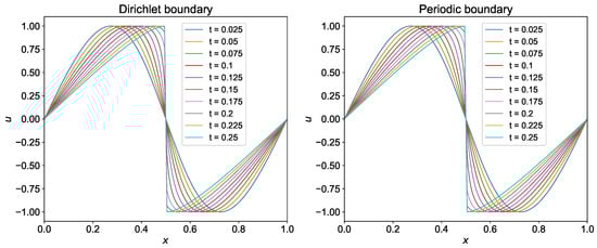
Figure 8. Evolution of shock with time for the initial condition $u_0=\sin (2\pi x)$ using WENO-5 scheme.

3.2. Compact Reconstruction WENO-5 Scheme

The main drawback of the WENO-5 scheme is that we have to increase the stencil size to get more accuracy. Compact reconstruction of WENO-5 scheme has been developed that uses smaller stencil without reducing the accuracy of the solution [25]. CRWENO-5 scheme uses compact stencils as their basis to calculate the left and right side state at the interface. The procedure for CRWENO-5 is similar to the WENO-5 scheme. However, its candidate stencils are implicit and hence smaller stencils can be used to get the same accuracy. The implicit system used to compute the left and right side state is given below

$$\begin{array}{cc}\hfill \left(\frac{2}{3}{w}_1^L+\frac{1}{3}{w}_2^L\right)u_{i-\frac{1}{2}}^L+\left[\frac{1}{3}{w}_1^L+\frac{2}{3}(w_2^L+w_3^L)\right]u_{i+\frac{1}{2}}^L+\frac{1}{3}{w}_3^L{u}_{i+\frac{3}{2}}^L& =\hfill \\ \hfill \frac{w_1^L}{6}{u}_{i-1}+\frac{5(w_1^L+w_2^L)+w_3^L}{6}{u}_i+\frac{w_2^L+5w_3^L}{6}{u}_{i+1},\end{array}$$

(44)

$$\begin{array}{cc}\hfill \frac{1}{3}{w}_3^R{u}_{i-\frac{1}{2}}^R+\left[\frac{1}{3}{w}_1^R+\frac{2}{3}(w_2^R+w_3^R)\right]u_{i+\frac{1}{2}}^R+\left(\frac{2}{3}{w}_1^R+\frac{1}{3}{w}_2^R\right)u_{i+\frac{3}{2}}^R& =\hfill \\ \hfill \frac{w_1^R}{6}{u}_{i-1}+\frac{5(w_1^R+w_2^R)+w_3^R}{6}{u}_i+\frac{w_2^R+5w_3^R}{6}{u}_{i+1},\end{array}$$

(45)

where the nonlinear weights are calculated using Equations (36) and (37), in which the linear weights are given by $d_0^L=1/5$, $d_1^L=1/2$, and $d_2^L=3/10$ in Equation (36), and $d_0^R=3/10$, $d_1^R=1/2$, and $d_2^R=1/5$ in Equation (37). The smoothness indicators are computed using Equations (38)–(40). The tridiagonal system formed using Equations (44) and (45) can be solved using the Thomas algorithm with $O(N)$ complexity, where N is the total number of grid points. In our implementation of CRWENO-5 scheme, we write a function that takes u in the candidate stencil (i.e., $u_{i-2},u_{i-1},u_i,u_{i+1},u_{i+2}$) and computes all coefficients in Equations (44) and (45). The implementation of Julia function to compute the coefficients of tridiagonal system for reconstruction of left side state is given in Listing 9. A similar function can be implemented for right side state also.

Listing 9. Implementation of Julia function to compute coefficients used for forming the implicit system in computation of left side numerical state at the interface.

We demonstrate CRWENO-5 scheme for both Dirichlet and periodic boundary condition. The Julia function to form the tridiagonal system for computing left side state at the interface in CRWENO-5 is given in Listing 10. We use a similar function for computing right side state.

Listing 10. Implementation of Julia function to form the tridiagonal system for computing left side numerical state at the interface for periodic boundary condition.

For periodic boundary condition, we use the relation given by Equation (43) for ghost points. The tridiagonal system formed for the periodic boundary condition is not purely tridiagonal and it has the following form

$$\underset{\phantom{(}\hat{\mathit{A}}}{\left[\begin{array}{ccccc}{b}_1& c_1& 0& \cdots & \beta \\ a_2& b_2& c_2& \cdots & 0\\ ⋮& ⋮& & \ddots & ⋮\\ 0& \cdots & a_{N-1}& b_{N-1}& c_{N-1}\\ \alpha & 0& \cdots & a_N& b_N\end{array}\right]}\underset{\phantom{(}\mathit{u}}{\left[\begin{array}{c}{u}_1\\ u_2\\ ⋮\\ u_{N-1}\\ u_N\end{array}\right]}=\underset{\phantom{(}\mathit{d}}{\left[\begin{array}{c}{d}_1\\ d_2\\ ⋮\\ d_{N-1}\\ d_N\end{array}\right]},$$

(46)

where $\hat{\mathit{A}}$ is the tridiagonal system, $\mathit{u}$ is the solution field and $\mathit{d}$ is the right hand side of the tridiagonal system. We use Sherman-Morrison formula [17] to solve the periodic tridiagonal system given in Equation (46). The Sherman-Morrison formula can be used to solve a sparse linear system of the equation if there is a faster way of calculating ${\mathit{A}}^{-1}$, where $\mathit{A}$ is the modified matrix without $\alpha$ and $\beta$. We can compute the ${\mathit{A}}^{-1}$ using the regular Thomas algorithm explained in Section 2.3. We can write Equation (46) as given below

$$(\mathit{A}+\mathit{p}\otimes \mathit{q})\mathit{u}=\mathit{d},$$

(47)

where

$$\mathit{p}=\underset{\phantom{(}}{\left[\begin{array}{c}\gamma \\ 0\\ ⋮\\ 0\\ \alpha \end{array}\right]},\mathit{q}=\underset{\phantom{(}}{\left[\begin{array}{c}1\\ 0\\ ⋮\\ 0\\ \beta /\gamma \end{array}\right]},$$

(48)

where $\gamma$ is arbitrary and the matrix $\mathit{A}$ is the tridiagonal part of the matrix $\hat{\mathit{A}}$, and ⊗ represents the outer product of two vectors. Then the solution to Equation (46) can be obtained using below formulas

$$\begin{array}{c}\hfill \mathit{A}·\mathit{y}=\mathit{d},\mathit{A}·\mathit{z}=\mathit{p},\end{array}$$

(49)

$$\begin{array}{c}\hfill \mathit{u}=\mathit{y}-\left[\frac{\mathit{q}·\mathit{y}}{1+\mathit{q}·\mathit{z}}\right]\mathit{z}.\end{array}$$

(50)

The cyclic Thomas algorithm for solving the periodic tridiagonal system is given in Algorithm 2.

Algorithm 2 Cyclic Thomas algorithm
1: Given $\mathit{a},\mathit{b},\mathit{c},\mathit{d},\alpha ,\beta$	▹ $\hat{\mathit{A}}\mathit{u}=\mathit{d}$
2: $\gamma =-b_1$	▹ Avoid subtraction error in forming $b{b}_0$
3: ${bb}_1=b_1-\gamma$, $b{b}_N=b_N-\alpha \beta /\gamma$	▹ Set up diagonal of the modified tridiagonal system
4: for $i=2$ to $N-1$ do
5:  $b{b}_i=b_i$
6: end for
7: Thomas($\mathit{a},\mathit{bb},\mathit{c},\mathit{d},\mathit{y}$)	▹ Solve $\mathit{A}·\mathit{y}=\mathit{d}$
8: $u_1=\gamma$, $u_N=\alpha$	▹ Set up the vector $\mathit{u}$
9: for $i=2$ to $N-1$ do
10:  $u_i=0.0$
11: end for
12: Thomas($\mathit{a},\mathit{bb},\mathit{c},\mathit{u},\mathit{z}$)	▹ Solve $\mathit{A}·\mathit{z}=\mathit{p}$
13: f = $(y_1+\beta y_N/\gamma )/(1.0+z_1+\beta z_N/\gamma )$	▹ Form $\mathit{q}·\mathit{y}/(1+\mathit{q}·\mathit{z})$
14: for $i=1$ to N do
15:  $u_i=y_i-f{z}_i$	▹ Calculate the solution vector $\mathit{u}$
16: end for

Once the left and right side states ($u^L,u^R$) are available we compute the right hand side term of the Burgers equation using Listing 7. We use third-order Runge-Kutta numerical scheme for time integration. We solve the tridiagonal system formed with periodic boundary condition using cyclic Thomas algorithm and for Dirichlet boundary condition, we use regular Thomas algorithm. The implementation of cyclic Thomas algorithm in Julia is given in Listing 11. The implementation of regular Thomas algorithm is given in Listing 4.

Listing 11. Implementation of cyclic Thomas algorithm in Julia for periodic boundary condition domain.

We test the CRWENO-5 method for the same problem as the WENO-5 scheme. The evolution of shock generated from sine wave with time is shown in Figure 9 for both Dirichlet and periodic boundary conditions computed using CRWENO-5 method. We use the same parameter as the WENO-5 scheme. We store snapshots of the solution field at different time steps to see the evolution of the shock. It can be seen from Figure 9 that the CRWENO-5 scheme captures the shock formed at final time $t=0.25$ accurately.

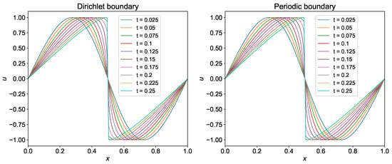
Figure 9. Evolution of shock with time for the initial condition $u_0=\sin (2\pi x)$ using CRWENO scheme.

4. Inviscid Burgers Equation: Conservative Form

In this section, we explain two approaches for solving the inviscid Burgers equation in its conservative form. The inviscid Burgers equation can be represented in the conservative form as below

$$\frac{\partial u}{\partial t}+\frac{\partial f}{\partial x}=0,\mathrm{where}f=\left(\frac{u^2}{2}\right).$$

(51)

The f is termed as the flux. We need to modify the grid arrangement to solve the inviscid Burgers equation in its conservative form. The modified grid for one-dimensional problem is shown in Figure 10. Here, $\Delta x=x_{i+1/2}-x_{i-1/2}$. The solution field is stored at the center of each cell and this type of grid is primarily used for finite volume discretization. We explain two approaches to compute the nonlinear term in the inviscid Burgers equation.

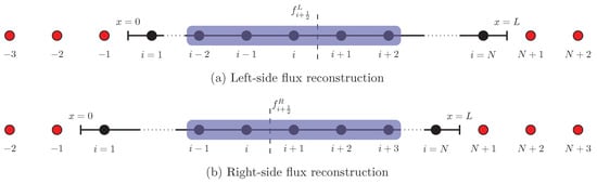
Figure 10. Finite difference grid for one-dimensional problems where the the solution is stored at the center of the cells. The flux is also computed at left and right boundary. The stencil required for reconstruction of left and right side flux is highlighted with blue rectangle. Ghost points are shown by red color.

4.1. Flux Splitting

The conservative form of the inviscid Burgers equation allows us to use the flux splitting method and WENO reconstruction to compute the flux at the interface. In this method, we first compute the flux f at the nodal points. The nonlinear advection term of the inviscid Burgers equation is computed as

$$\begin{array}{cc}\hfill \frac{\partial f}{\partial x}{|}_{x=x_i}& =\frac{f_{i+1/2}-f_{i-1/2}}{\Delta x},\hfill \end{array}$$

(52)

$$\begin{array}{cc}\hfill \frac{\partial f}{\partial x}{|}_{x=x_i}& =\frac{f_{i+1/2}^L-f_{i-1/2}^L}{\Delta x}+\frac{f_{i+1/2}^R-f_{i-1/2}^R}{\Delta x},\hfill \end{array}$$

(53)

at a particular node i. The superscripts L and R refer to the positive and negative flux component at the interface and the subscripts $i-1/2$ and $i+1/2$ stands for the left and right side interface of the nodal point i. We use WENO-5 reconstruction discussed in Section 3.1 to compute the left and right side flux at the interface. First, we compute the flux at nodal points and then split it into positive and negative components. This process is called as Lax-Friedrichs flux splitting and the positive and negative component of the flux at a nodal location is calculated as

$$f_i^{+}=\frac{1}{2}(f_i+\alpha u_i),f_i^{-}=\frac{1}{2}(f_i-\alpha u_i),$$

(54)

where $\alpha$ is the absolute value of the flux Jacobian ($\alpha =|\frac{\partial f}{\partial u}|$). We chose the values of $\alpha$ as the maximum value of $u_i$ over the stencil used for WENO-5 reconstruction, i.e.,

$$\alpha =\max (|u_{i-2}|,|u_{i-1}|,|u_i|,|u_{i+1}|,|u_{i+2}|).$$

(55)

Once we split the nodal flux into its positive and negative component we reconstruct the left and right side fluxes at the interface using WENO-5 scheme using below formulas [24]

$$\begin{array}{c}\hfill f_{i+\frac{1}{2}}^L=w_0^L\left(\frac{1}{3}{f}_{i-2}^{+}-\frac{7}{6}{f}_{i-1}^{+}+\frac{11}{6}{f}_i^{+}\right)+w_1^L\left(-\frac{1}{6}{f}_{i-1}^{+}+\frac{5}{6}{f}_i^{+}+\frac{1}{3}{f}_{i+1}^{+}\right)+w_2^L\left(\frac{1}{3}{f}_i^{+}+\frac{5}{6}{f}_{i+1}^{+}-\frac{1}{6}{f}_{i+2}^{+}\right),\end{array}$$

(56)

$$\begin{array}{c}\hfill f_{i-\frac{1}{2}}^R=w_0^R\left(-\frac{1}{6}{f}_{i-2}^{-}+\frac{5}{6}{f}_{i-1}^{-}+\frac{1}{3}{f}_i^{-}\right)+w_1^R\left(\frac{1}{3}{f}_{i-1}^{-}+\frac{5}{6}{f}_i^{-}-\frac{1}{6}{f}_{i+1}^{-}\right)+w_2^R\left(\frac{11}{6}{f}_i^{-}-\frac{7}{6}{f}_{i+1}^{-}+\frac{1}{3}{f}_{i+2}^{-}\right),\end{array}$$

(57)

where the nonlinear weights are computed using Equations (36) and (37). Once we have left and right side fluxes at the interface we use Equation (53) to compute the flux derivative. We demonstrate the flux splitting method for a shock generated by sine wave similar to Section 3. We use the third-order Runge-Kutta numerical scheme for time integration and periodic boundary condition for the domain. For the conservative form, we need three ghost points on left and right sides, since we compute the flux at the left and right boundary of the domain also. The periodic boundary condition for fluxes at ghost points is given by

$$f_{-3}=f_{N-2},f_{-2}=f_{N-1},f_{-1}=f_N,f_{N+1}=f_1,f_{N+2}=f_2,f_{N+3}=f_3.$$

(58)

The Julia function to compute the right hand side of the inviscid Burgers equation is detailed in Listing 12. The implementation of flux reconstruction and weight computation in Julia is similar to Listings 6 and 8.

Listing 12. Implementation of Julia function to calculate the right hand side of inviscid Burgers equation using flux splitting method.

4.2. Riemann Solver: Rusanov Scheme

Another approach to computing the nonlinear term in the inviscid Burgers equation is to use Riemann solvers. Riemann solvers are used for accurate and efficient simulations of Euler equations along with higher-order WENO schemes [27,28]. In this method, first, we reconstruct the left and right side fluxes at the interface similar to the inviscid Burgers equation in non-conservative form. Once we have $f_{i+1/2}^L$ and $f_{i+1/2}^R$ reconstructed, we use Riemann solvers to compute the fluxes at the interface. We follow the same procedure discussed in Section 3.1 to reconstruct the fluxes at the interface. We can also use CRWENO-5 scheme presented in Section 3.2 to determine the fluxes.

We use a simple Rusanov scheme as the Riemann solver [29]. The Rusanov scheme uses maximum local wave propagation speed to compute the flux as follows

$$f_{i+1/2}=\frac{1}{2}\left(f_{i+1/2}^L+f_{i+1/2}^R\right)-\frac{c_{i+1/2}}{2}\left(u_{i+1/2}^L-u_{i+1/2}^R\right),$$

(59)

where $f^L$ is the flux component using the right reconstructed state $f_{i+1/2}^L=f(u_{i+1/2}^L)$, and $f^R$ is the flux component using the right reconstructed state $f_{i+1/2}^R=f(u_{i+1/2}^R)$. Here, $c_{i+1/2}$ is the local wave propagation speed which is obtained by taking the maximum absolute value of the eigenvalues corresponding to the Jacobian, $\frac{\partial f}{\partial u}=u$, between cells i and $i+1$ can be obtained as

$$c_{i+1/2}=\max (|u_i|,|u_{i-1}|),$$

(60)

or in a wider stencil as shown in Equation (55). The implementation of Riemann solver with Rusanov scheme for inviscid Burgers equation is given in Listing 13. The implementation of state reconstruction and weight computation in Julia is similar to Listings 6 and 8. Figure 11 shows the evolution of shock for the sine wave. We use the same parameters for the spatial and temporal discretization of the inviscid Burgers equation as used for the non-conservative form in Section 3.

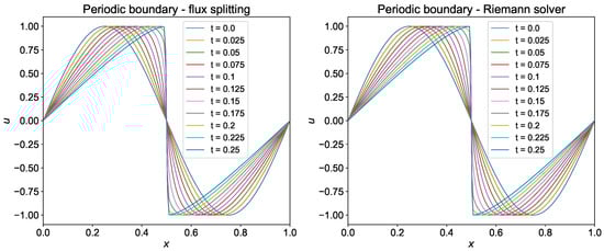
Figure 11. Evolution of shock from sine wave ($u_0=\sin (2\pi x)$) computed using conservative form of inviscid Burgers equation. The reconstruction of the field is done using WENO-5 scheme, and flux splitting and Riemann solver approach is used to compute the nonlinear term.

Listing 13. Implementation of Julia function to calculate the right hand side of inviscid Burgers equation using Riemann solver based on Rusanov scheme.

5. One-Dimensional Euler Solver

In this section, we present a solution to one-dimensional Euler equations. Euler equations contain a set of nonlinear hyperbolic conservation laws that govern the dynamics of compressible fluids neglecting the effect of body forces, and viscous stress [30]. The one-dimensional Euler equations in its conservative form can be written as

$$\frac{\partial q}{\partial t}+\frac{\partial F}{\partial x}=0,$$

(61)

where

$$q=\left(\begin{array}{c}\rho \\ \rho u\\ \rho e\end{array}\right),F=\left(\begin{array}{c}\rho u\\ \rho u^2+p\\ \rho uh\end{array}\right),$$

in which

$$h=e+\frac{p}{\rho },p=\rho (\gamma -1)\left(e-\frac{1}{2}{u}^2\right).$$

(62)

Here, $\rho$ and p are the density, and pressure respectively; u is the horizontal component of velocity; e and h stand for the internal energy and static enthalpy, and $\gamma$ is the ratio of specific heats. Equation (61) can also be written as

$$\frac{\partial q}{\partial t}+A\frac{\partial q}{\partial x}=0,$$

(63)

where $A=\frac{\partial F}{\partial q}$ is the convective flux Jacobian matrix. The matrix A is given as

$$A=\frac{\partial F}{\partial q}=\left(\begin{array}{ccc}0& 1& 0\\ {\varphi }^2-u^2& (3-\gamma )u& \gamma -1\\ ({\varphi }^2-h)u& h-(\gamma -1)u^2& \gamma u\end{array}\right),$$

(64)

where ${\varphi }^2=\frac{1}{2}(\gamma -1)u^2$. We can write the matrix A as $A=R\mathsf{\Lambda }L$ in which Λ is the diagonal matrix of real eigenvalues of A, i.e., $\mathsf{\Lambda }=\mathrm{diag}[u,u+a,u-a]$. Here, L and R are the matrices of which the columns are the left and right eigenvectors of A; $L=R^{-1}$. The matrices L and R are given below [31]

$$L=\left(\begin{array}{ccc}1-\frac{{\varphi }^2}{a^2}& (\gamma -1)\frac{u}{a^2}& -\frac{(\gamma -1)}{a^2}\\ {\varphi }^2-ua& a-(\gamma -1)u& \gamma -1\\ {\varphi }^2+ua& -a-(\gamma -1)u& \gamma -1\end{array}\right),R=\left(\begin{array}{ccc}1& \beta & \beta \\ u& \beta (u+a)& \beta (u-a)\\ \frac{{\varphi }^2}{(\gamma -1)}& \beta (h+ua)& \beta (h-ua)\end{array}\right),$$

(65)

where a is the speed of sound and is given by $a^2=\gamma p/\rho$, and $\beta =1/(2a^2)$.

We use the grid similar to the one used for the conservative form of the inviscid Burgers equation and is shown in Figure 10. The semi-discrete form of the Euler equations can be written as

$$\frac{\partial q_i}{\partial t}+\frac{F_{i+1/2}-F_{i-1/2}}{\Delta x}=0,$$

(66)

where $q_i$ is the cell-centered values stored at nodal points and $F_{i\pm 1/2}$ are the fluxes at left and right cell interface. We use third-order Runge-Kutta numerical method for time integration. We use WENO-5 reconstruction to compute the left and sight states of the fluxes at the interface. We include three different Riemann solvers to compute the flux $F_{i\pm 1/2}$ at interfaces to be used in Equation (66).

5.1. Roe’s Riemann Solver

First, we present the Roe solver for one-dimensional Euler equations. According to the Gudanov theorem [32], for a hyperbolic system of equations, if the Jacobian matrix of the flux vector is constant (i.e., $A=\frac{\partial F}{\partial q}=\mathrm{constant}$), the exact values of fluxes at the interfaces can be calculated as

$$F_{i+1/2}=\frac{1}{2}\left(F_{i+1/2}^R+F_{i+1/2}^L\right)-\frac{1}{2}R\left|\mathsf{\Lambda }\right|L\left(q_{i+1/2}^R-q_{i+1/2}^L\right),$$

(67)

where |Λ| is the diagonal matrix consisting of absolute values eigenvalues of the Jacobian matrix and the matrices L and R are given in Equation (65). However, Jacobian matrix is not constant (i.e., $F=F(q)$). The Roe solver [33] is an approximate Riemann solver and it uses below formulation to find the numerical fluxes at the interface

$$F_{i+1/2}=\frac{1}{2}\left(F_{i+1/2}^R+F_{i+1/2}^L\right)-\frac{1}{2}\overline{R}\left|\overline{\mathsf{\Lambda }}\right|\overline{L}\left(q_{i+1/2}^R-q_{i+1/2}^L\right),$$

(68)

where the bar represents the Roe average between the left and right states. In order to derive $\overline{A}$ we need to know $\overline{u}$, $\overline{h}$, and $\overline{a}$ and they are computed using Roe averaging procedure. In order to derive $\overline{u}$, $\overline{h}$, and $\overline{a}$ Roe used Taylor series expansion of F around $q^L$ and $q^R$ points.

$$\begin{array}{cc}\hfill F(q)& =F(q^L)+A(q^L)(q-q^L),\hfill \end{array}$$

(69)

$$\begin{array}{cc}\hfill F(q)& =F(q^R)+A(q^R)(q-q^R).\hfill \end{array}$$

(70)

Neglecting higher-order terms and equation above two equations

$$F(q^L)-F(q^R)=A(q^L-q^R)+\left(A(q^R)-A(q^L)\right)q.$$

(71)

Roe [20] derived approximate matrix $\overline{A}$ such that it satisfies $\overline{A}(q^L,q^R)\to A(q)$ as $\overline{q}\to q$. Therefore, we get the following set of equations (written in vector form)

$$F(q^L)-F(q^R)=\overline{A}(q^L-q^R).$$

(72)

Using Equation (72) we can compute $\overline{u}$, $\overline{h}$, and $\overline{a}$. First we reconstruct the left and right states of q at the interface (i.e., $q_{i+1/2}^R$ and $q_{i+1/2}^L$) using WENO-5 scheme. Then, we can compute the left and right state of the fluxes (i.e., $F^L$ and $F^R$) using Equation (61). The Roe averaging formulas to compute approximate values for constructing $\overline{R}$ and $\overline{L}$ are given below

$$\begin{array}{cc}\hfill \overline{u}& =\frac{u_R\sqrt{{\rho }_R}+u_L\sqrt{{\rho }_L}}{\sqrt{{\rho }_R}+\sqrt{{\rho }_L}},\hfill \end{array}$$

(73)

$$\begin{array}{cc}\hfill \overline{h}& =\frac{h_R\sqrt{{\rho }_R}+h_L\sqrt{{\rho }_L}}{\sqrt{{\rho }_R}+\sqrt{{\rho }_L}},\hfill \end{array}$$

(74)

where the left and right states are computed using WENO-5 reconstruction. The speed of the sound is computed using the below equation

$$\overline{a}=\sqrt{(\gamma -1)\left[\overline{h}-\frac{1}{2}{\overline{u}}^2\right]}.$$

(75)

The eigenvalues of the Jacobian matrix are ${\lambda }_1=\overline{u}$, ${\lambda }_2=\overline{u}+a$, and ${\lambda }_3=\overline{u}-a$. The implementation of Roe’s Riemann solver is given in Listing 14.

Listing 14. Implementation of Julia function to calculate the right hand side of Euler equations using Roe’s Riemann solver.

The implementation of WENO-5 reconstruction is similar to Listings 8 and 9. We implemented all Riemann solvers for Euler equations in such a way that we compute smoothness indicators for all equations separately. We do not incur much computational expense since our problem is one-dimensional. However, for higher-dimension usually smoothness indicator is computed only for equation (usually momentum or energy equation) and the same smoothness indicators are used for all equations. The computation of flux using Roe averaging is detailed in Listing 15.

Listing 15. Implementation of Julia function to calculate the interface flux using Riemann solver based on Roe averaging.

We test the Riemann solver using Sod shock tube problem [34]. The time evolution of Sod shock tube problem is governed buy Euler equations. This problem is used for testing numerical schemes to study how well they can capture and resolve shocks and discontinuities and their ability to produce correct density profile. The initial conditions for the Sod shock tube problem are

$$\left(\begin{array}{c}{\rho }_L\\ p_L\\ u_L\end{array}\right)=\left(\begin{array}{c}1.0\\ 1.0\\ 0.0\end{array}\right)\mathrm{when}x<0.5;\left(\begin{array}{c}{\rho }_R\\ p_R\\ u_R\end{array}\right)=\left(\begin{array}{c}0.125\\ 0.1\\ 0.0\end{array}\right)\mathrm{when}x>0.5.$$

(76)

We use third-order Runge-Kutta numerical scheme for time integration from $t=0$ to $t=0.2$. We use two grid resolutions to see the capability of Riemann solver to capture the shock. The Sod shock tube problem has Dirichlet boundary condition at the left and right boundary. We use linear interpolation to find the values of q at ghost points. Figure 12 shows the density, velocity, pressure, and energy at final time $t=0.2$ using Roe solver. We consider the solution obtained with high-grid resolution as the true solution and compare it with the low-resolution results. From Figure 12, we observe that there are small oscillations near discontinuities at low-resolution. We use WENO reconstruction to compute the flux at interface and WENO scheme is not strictly non-oscillatory. However, WENO scheme does not allow oscillations to amplify to large values. To remove these oscillations further, for example, we can use characteristic-wise reconstructions [35].

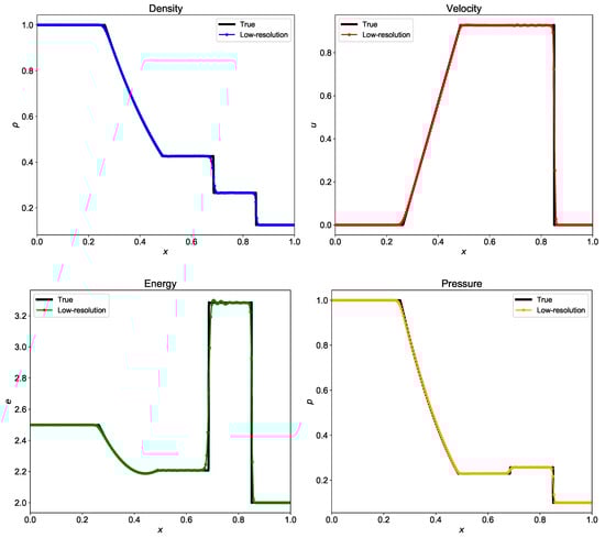
Figure 12. Evolution of density, velocity, energy, and pressure at $t=0.2$ for the shock tube problem computed using Riemann solver based on Roe averaging. The true solution is calculated with $N=8192$ grid resolution with $\Delta t=0.00005$ and the low-resolution results are for $N=256$ grid resolution with $\Delta t=0.0001$.

5.2. HLLC Riemann Solver

We present one of the most widely used approximate Riemann solver based on HLLC scheme [30,36]. They used lower and upper bounds on the characteristics speeds in the solution of Riemann problem involving left and right states. These bounds are approximated as

$$\begin{array}{cc}\hfill S_L& =\min (u_L,u_R)-\max (a_L,a_R),\hfill \end{array}$$

(77)

$$\begin{array}{cc}\hfill S_R& =\min (u_L,u_R)+\max (a_L,a_R),\hfill \end{array}$$

(78)

where $S_L$ and $S_R$ are the lower and upper bound for the left and right state characteristics speed. For HLLC scheme we also include middle wave of speed $S_{*}$ given by

$$S_{*}=\frac{p_R-p_L+{\rho }_L{u}_L(S_L-u_L){\rho }_R{u}_R(S_R-uR)}{{\rho }_L(S_L-u_L)-{\rho }_R(S_R-u_R)}.$$

(79)

The mean pressure is given by

$$P_{LR}=\frac{1}{2}\left[p_L+p_R+{\rho }_L(S_L-u_L)(S_{*}-u_l)+{\rho }_R(S_R-u_R)(S_{*}-u_R)\right].$$

(80)

The fluxes are computed as

$$F_{i+1/2}=\left\{\begin{array}{cc}{F}^L,\hfill & \mathrm{if} S_L\ge 0\hfill \\ F^R,\hfill & \mathrm{if} S_R\le 0\hfill \\ \frac{S_{*}(S_L{u}_L{F}^L)+S_L{P}_{LR}{D}_{*}}{S_L-S_{*}},\hfill & \mathrm{if} S_L\le 0 \mathrm{and} S_{*}\ge 0\hfill \\ \frac{S_{*}(S_R{u}_R{F}^R)+S_R{P}_{LR}{D}_{*}}{S_R-S_{*}},\hfill & \mathrm{if} S_R\ge 0 \mathrm{and} S_{*}\le 0\hfill \end{array}\right.$$

(81)

where $D_{*}=[0,1,S_{*}]$. Once the flux is available at the interface, we can integrate the solution in time using Equation (66). The implementation of HLLC scheme is given in Listing 16. We perform the time integration using third-order Runge-Kutta numerical scheme. Figure 13 shows the density, velocity, pressure, and energy at final time $t=0.2$ computed using Riemann solver based on HLLC scheme. The oscillations in the numerical solution calculated by the HLLC scheme is slightly less than those calculated by the Roe’s Riemann solver. The true solution is computed using $N=8192$ grid points and $\Delta t=0.00005$ and is compared with the low-resolution results for $N=256$ grid points and $\Delta t=0.0001$.

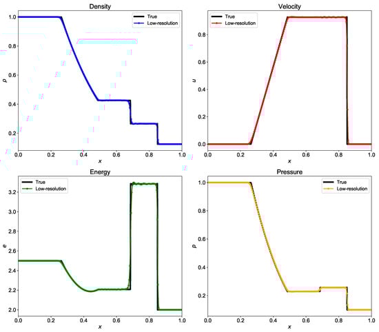
Figure 13. Evolution of density, velocity, energy, and pressure at $t=0.2$ for the shock tube problem computed using Riemann solver based on Harten-Lax-van Leer Contact (HLLC) scheme. The true solution is calculated with $N=8192$ grid resolution with $\Delta t=0.00005$ and the low-resolution results are for $N=256$ grid resolution with $\Delta t=0.0001$.

Listing 16. Implementation of Julia function to calculate the interface flux using Riemann solver based on HLLC scheme.

5.3. Rusanov’s Riemann Solver

We show the implementation of Riemann solver using Rusanov scheme. This is similar to what we discussed in Section 4.2. The Riemann solver based on Rusanov scheme is simple compared to Roe’s Riemann solver and HLLC based Riemann solver. For Euler equations, instead of solving one equation (as in inviscid Burgers equation), now we have to follow the procedure for three equations (i.e., density, velocity, and energy). We need to approximate wave propagation speed at the interface $c_{i+1/2}$ to compute flux at the interface. For Rusanov scheme, we simply use maximum eigenvalue of the Jacobian matrix as the wave propagation speed. We have $c_{i+1/2}=max(\overline{u},|\overline{u}+\overline{a}|,|\overline{u}-\overline{a}|)$, where $\overline{u}$ and $\overline{a}$ are computed using Roe averaging. Figure 14 shows the density, velocity, pressure, and energy at final time $t=0.2$ computed using Riemann solver based on Rusanov scheme. The oscillations in the numerical solution calculated by the Rusanov scheme is more than those calculated by the Roe’s Riemann solver or HLLC scheme based Riemann solver. One of the advantage of Rusanov scheme is that it is simple to implement and is computationally faster. The true solution is computed using $N=8192$ grid points and $\Delta t=0.00005$ and is compared with the low-resolution results for $N=256$ grid points and $\Delta t=0.0001$. The implementation of Riemann solver based on Rusanov’s scheme is given in Listing 17.

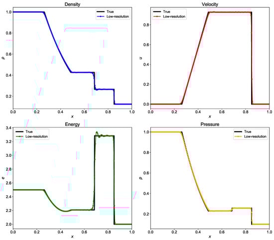
Figure 14. Evolution of density, velocity, energy, and pressure at $t=0.2$ for the shock tube problem computed using Riemann solver based on Rusanov scheme. The true solution is calculated with $N=8192$ grid resolution with $\Delta t=0.00005$ and the low-resolution results are for $N=256$ grid resolution with $\Delta t=0.0001$.

Listing 17. Implementation of Julia function to calculate the interface flux using Riemann solver based on Rusanov scheme.

6. Two-Dimensional Poisson Equation

In this section, we explain different methods to solve the Poisson equation which is encountered in solution to the incompressible flows. The Poisson equation is solved at every iteration step in the solution to the incompressible Navier-Stokes equation due to the continuity constraint. Therefore, many studies have been done to accelerate the solution to the Poisson equation using higher-order numerical methods [37], and developing fast parallel algorithms [38]. The Poisson equation is a second-order elliptic equation and can be represented as

$$\frac{{\partial }^{2}u}{\partial x^2}+\frac{{\partial }^{2}u}{\partial y^2}=f.$$

(82)

Using the second-order central difference formula for discretization of the Poisson equation, we get

$$\frac{u_{i+1,j}-2u_{i,j}+u_{i-1,j}}{{\Delta x}^2}+\frac{u_{i,j+1}-2u_{i,j}+u_{i,j-1}}{{\Delta y}^2}=f_{i,j},$$

(83)

where $\Delta x$ and $\Delta y$ is the grid spacing in the x and y directions, and $f_{i,j}$ is the source term at discrete grid locations. If we write Equation (83) at each grid point, we get a system of linear equations. For the Dirichlet boundary condition, we assume that the values of $u_{i,j}$ are available when $(x_i,y_j)$ is a boundary point. These equations can be written in the standard matrix notation as

$$\underset{\phantom{(}A}{\left[\begin{array}{cccccccc}{D}_{xy}& D_y& 0& \cdots & D_x& \cdots & \cdots & 0\\ D_y& D_{xy}& D_y& \ddots & & \ddots & & ⋮\\ 0& D_y& D_{xy}& D_y& \ddots & & \ddots & ⋮\\ ⋮& \ddots & \ddots & \ddots & \ddots & \ddots & & D_x\\ D_x& & \ddots & \ddots & \ddots & \ddots & \ddots & ⋮\\ ⋮& \ddots & & \ddots & D_y& D_{xy}& D_y& 0\\ ⋮& & \ddots & & \ddots & D_y& D_{xy}& D_y\\ 0& \cdots & \cdots & D_x& \cdots & 0& D_y& D_{xy}\end{array}\right]}\underset{\phantom{(}\mathit{u}}{\left[\begin{array}{c}{u}_{1,1}\\ u_{1,2}\\ ⋮\\ ⋮\\ u_{2,1}\\ ⋮\\ ⋮\\ u_{N_x,N_y}\end{array}\right]}=\underset{\phantom{(}\mathit{b}}{\left[\begin{array}{c}{f}_{1,1}\\ f_{1,2}\\ ⋮\\ ⋮\\ f_{2,1}\\ ⋮\\ ⋮\\ f_{N_x,N_y}\end{array}\right]},$$

(84)

where

$$D_{xy}=\frac{-2}{{\Delta x}^2}+\frac{-2}{{\Delta y}^2};D_x=\frac{1}{{\Delta x}^2};D_y=\frac{1}{{\Delta y}^2}.$$

The boundary points of the domain are incorporated in the source term vector $\mathit{b}$ in Equation (84). We can solve Equation (84) by standard methods for systems of linear equations, such as Gaussian elimination [39]. However, the matrix A is very sparse and the standard methods are computationally expensive for large size of A. In this paper, we discuss direct methods based on fast Fourier transform (FFT) and fast sine transform (FST) for periodic and Dirichlet boundary condition. We also explain iterative methods to solve Equation (84). We will further present a multigrid framework which scales linearly with a number of discrete grid points in the domain.

6.1. Direct Solver

Figure 15 shows the finite difference grid for two-dimensional CFD problems. We use two different boundary conditions for direct Poisson solver: periodic and Dirichlet boundary condition. For the Dirichlet boundary condition, the nodal values of a solution are already known and do not change, and hence, we do not do any calculation for the boundary points. In case of periodic boundary condition, we do calculation for grid points $(i,j)$ between $[1,N_x]\times [1,N_y]$. The solution at right $(i=N_x+1)$ and top $(j=N_y+1)$ boundary is obtained from left $(i=1)$ and bottom $(j=1)$ boundary, respectively.

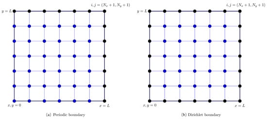
Figure 15. Finite difference grid for two-dimensional problems. The calculation is done only for points shown by blue color. The solution at black points is extended from left and bottom boundary for periodic boundary condition. The solution is already available at all four boundaries for Dirichlet boundary condition.

We perform the assessment of direct solver using the method of manufactured solution. We assume certain field u and compute the source term f at each grid location. We then solve the Poisson equation for this source term f and compare the numerically calculated field u with the exact solution field u. The exact field u and the corresponding source term f used for direct Poisson solver are given below

$$\begin{array}{c}\hfill u(x,y)=\sin (2\pi x)\sin (2\pi y)+\frac{1}{{16}^2}\sin (32\pi x)\sin (32\pi y),\end{array}$$

(85)

$$\begin{array}{c}\hfill f(x,y)=-8{\pi }^2\sin (2\pi x)\sin (2\pi y)-8{\pi }^2\sin (32\pi x)\sin (32\pi y).\end{array}$$

(86)

This problem can have both periodic and Dirichlet boundary conditions. The computational domain is square in shape and is divided into 512 × 512 grid in x and y directions.

6.1.1. Fast Fourier Transform

There are two different ways to implement fast Poisson solver for the periodic domain. One way is to perform FFTs directly on the Poisson equation, which will give us the spectral accuracy. The second method is to discretize the Poisson equation first and then apply FFTs on the discretized equation. The second approach will give us the same spatial order of accuracy as the numerical scheme used for discretization. We use the second-order central difference scheme given in Equation (83) for developing a direct Poisson solver.

The Fourier transform decomposes a spatial function into its sine and cosine components. The output of the Fourier transform is the function in its frequency domain. We can recover the function from its frequency domain using the inverse Fourier transform. We use both the function and its Fourier transform in the discretized domain which is called the discrete Fourier transform (DFT). Cooley-Tukey proposed an FFT algorithm that reduces the complexity of computing DFT from $O(N^2)$ to $O(N\log N)$, where N is the data size [17]. In two-dimensions, the DFT for a square domain discretized equally in both directions is defined as

$${\tilde{u}}_{m,n}=\sum _{i=0}^{N_x-1}\sum _{j=0}^{N_y-1}{u}_{i,j}{e}^{-\iota 2\pi \left(\frac{mi}{N_x}+\frac{nj}{N_y}\right)},$$

(87)

where $u_{i,j}$ is the function in the spatial domain and the exponential term is the basis function corresponding to each point ${\tilde{u}}_{m,n}$ in the Fourier space, m and n are the wavenumbers in Fourier space in x and y directions, respectively. This equation can be interpreted as the value in the frequency domain ${\tilde{u}}_{m,n}$ can be obtained by multiplying the spatial function with the corresponding basis function and summing the result. The basis functions are sine and cosine waves with increasing frequencies. Here, ${\tilde{u}}_{0,0}$ represents the component of the function with the lowest wavenumber and ${\tilde{u}}_{N_x-1,N_y-1}$ represents the component with the highest wavenumber. Similarly, the function in Fourier space can be transformed to the spatial domain. The inverse discrete Fourier transform (IDFT) is given by

$$u_{i,j}=\frac{1}{N_x}\frac{1}{N_y}\sum _{m=-N_x/2}^{N_x/2-1}\sum _{n=-N_y/2}^{N_y/2-1}{\tilde{u}}_{m,n}{e}^{\iota 2\pi \left(\frac{mi}{N_x}+\frac{nj}{N_y}\right)},$$

(88)

where $1/(N_x{N}_y)$ is the normalization term. The normalization can also be applied to forward transform, but it should be used only once. If we use Equation (88) in Equation (83), we get

$$\begin{array}{cc}\hfill {\tilde{u}}_{m,n}\left(\frac{e^{\iota \frac{2\pi m}{N_x}}-2+e^{\iota \frac{-2\pi m}{N_x}}}{\Delta x^2}+\frac{e^{\iota \frac{2\pi n}{N_y}}-2+e^{\iota \frac{-2\pi n}{N_y}}}{\Delta y^2}\right)& ={\tilde{f}}_{m,n},\hfill \end{array}$$

(89)

in which we use the definition of cosine to yield

$$\begin{array}{cc}\hfill {\tilde{u}}_{m,n}\left(\frac{2\cos \left(\frac{2\pi m}{N_x}\right)-2}{\Delta x^2}+\frac{2\cos \left(\frac{2\pi n}{N_y}\right)-2}{\Delta y^2}\right)& ={\tilde{f}}_{m,n}.\hfill \end{array}$$

(90)

If we take the forward DFT of Equation (90), we get a spatial function $u_{i,j}$. The three step procedure to develop a Poisson solver using FFT is given below

• Apply forward FFT to find the Fourier coefficients of the source term in the Poisson equation (${\tilde{f}}_{m,n}$ from the grid values $f_{i,j}$)
• Get the Fourier coefficients for the solution ${\tilde{u}}_{m,n}$ using below relation

  $${\tilde{u}}_{m,n}=\frac{{\tilde{f}}_{m,n}}{\left(\frac{2}{\Delta x^2}\cos \left(\frac{2\pi m}{N_x}\right)+\frac{2}{\Delta y^2}\cos \left(\frac{2\pi n}{N_y}\right)-\frac{2}{\Delta x^2}-\frac{2}{\Delta y^2}\right)}.$$

  (91)
• Apply inverse FFT to get the grid values $u_{i,j}$ from the Fourier coefficients ${\tilde{u}}_{m,n}$.

Implementation of Poisson solver using FFT is given in Listing 18. Figure 16 shows the exact and numerical solution for for the test problem.

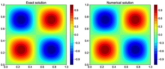
Figure 16. Comparison of exact solution and numerical solution computed using fast Fourier transform method for the Poisson equation with periodic boundary condition.

Listing 18. Implementation of Julia function for the Poisson solver using fast Fourier transform (FFT) for the domain with periodic boundary condition.

We develop the Poisson solver using a second-order central difference scheme for discretization of the Poisson equation. Instead of using the discretized equation, we can directly use Fourier analysis for the Poisson equation. This will compute the exact solution and the solution will not depend upon the grid size. The only change will be the change in Equation (91). We can easily derive the equation for Fourier coefficients in spectral solver by performing forward FFT of Equation (82). The Fourier coefficients for spectral solver can be written as

$${\tilde{u}}_{m,n}=-\frac{{\tilde{f}}_{m,n}}{m^2+n^2}.$$

(92)

We can get the solution by performing inverse FFT of the above equation. The implementation of spectral Poisson solver in Julia is outlined in Listing 19.

Listing 19. Implementation of Julia function for the spectral Poisson solver using fast Fourier transform (FFT) for the domain with periodic boundary condition.

The spectral Poisson solver gives the exact solution and the error between exact and numerical solution is machine zero error. We demonstrate it by using spectral Poisson solver for three different grid resolutions. We also use the central-difference scheme (CDS) Poisson solver at these grid resolutions and compare the discretization errors for two methods. We systematically change the grid spacing by a factor of two in both x and y direction and compute the $L_2$ norm of the discretization error. Figure 17 shows the contour plot for the error at three grid resolutions for spectral and second-order CDS. We can notice that the error for the spectral method does not depend on the grid resolution and the value of error is of the same order as machine zero error. On the other hand, for CDS the error reduces as we increase the grid resolution. This is because the truncation error goes down with the decrease in grid spacing. Figure 18 plots the $L_2$ norm of the error for spectral method and CDS. The slope of the discretization error is two for CDS showing that the scheme has second-order of accuracy. This method is used in CFD to validate the code and numerical methods. For the spectral method, the $L_2$ norm of the error has the machine zero value for all three grid resolutions.

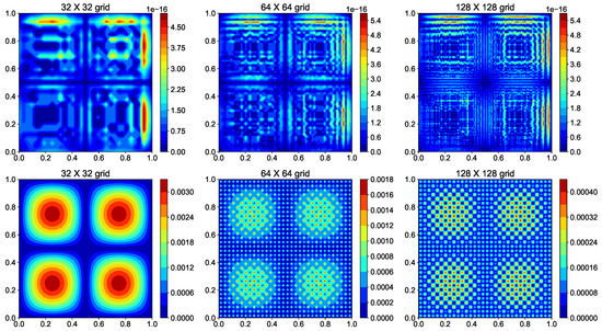
Figure 17. Comparison of error for spectral method (Top) and second-order CDS (bottom) for three different grid resolutions. The error is defined as $ϵ(x,y)=|u^{exact}-u^{numerical}|$.

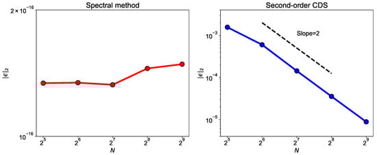
Figure 18. Order of accuracy for spectral method and second-order CDS. We calculate discretization error at five grid resolutions and change the grid size by a factor of 2 in both x and y direction. The CDS Poisson solver give second-order accuracy. Spectral method give exact solution and error is of the same order as machine zero.

6.1.2. Fast Sine Transform

The procedure described in Section 6.1.1 is valid only when the problem has periodic boundary condition, i.e., the solution that satisfies $u_{i,j}=u_{i+N_x,j}=u_{i,j+N_y}$. If we have homogeneous Dirichlet boundary condition for the square domain problem, we need to use the sine transform given by

$${\tilde{u}}_{m,n}=\sum _{i=0}^{N_x-1}\sum _{j=0}^{N_x-1}{u}_{i,j}\sin \frac{\pi mi}{N_x}\sin \frac{\pi nj}{N_y},$$

(93)

where m and n are the wavenumbers. This satisfies the homogeneous Dirichlet boundary conditions that $u=0$ at $i=0,N_x$ and $j=0,N_y$. If we substitute Equation (93) in Equation (83) and use trigonometric identity ($\sin (A\pm B)=\sin (A)\cos (B)\pm \sin (B)\cos (A)$) we get

$${\tilde{u}}_{m,n}\left(\frac{2\cos \left(\frac{\pi m}{N_x}\right)-2}{\Delta x^2}+\frac{2\cos \left(\frac{\pi n}{N_y}\right)-2}{\Delta y^2}\right)={\tilde{f}}_{m,n}.$$

(94)

We can compute the spatial field using inverse sine transform given by

$$u_{i,j}=\frac{2}{N_x}\frac{2}{N_y}\sum _{m=0}^{N_x-1}\sum _{n=0}^{N_y-1}{\tilde{u}}_{m,n}\sin \frac{\pi mi}{N_x}\sin \frac{\pi nj}{N_y}.$$

(95)

The three-step procedure to develop Poisson solver using sine transform can be listed as

• Apply forward sine transform to find the Fourier coefficients of the source term in the Poisson equation (${\tilde{f}}_{m,n}$ from the grid values $f_{i,j}$)
• Get the Fourier coefficients for the solution ${\tilde{u}}_{m,n}$ using below relation

  $${\tilde{u}}_{m,n}=\frac{{\tilde{f}}_{m,n}}{\left(\frac{2}{\Delta x^2}\cos \left(\frac{\pi m}{N_x}\right)+\frac{2}{\Delta y^2}\cos \left(\frac{\pi n}{N_y}\right)-\frac{2}{\Delta x^2}-\frac{2}{\Delta y^2}\right)}.$$

  (96)
• Apply inverse sine transform to get the grid values $u_{i,j}$ from the Fourier coefficients ${\tilde{u}}_{m,n}$.

The implementation of Poisson solver for problems with homogeneous Dirichlet boundary condition using the sine transform is given in Listing 20. Figure 19 displays the comparison of exact and numerical solution for the test problem computed using sine transform.

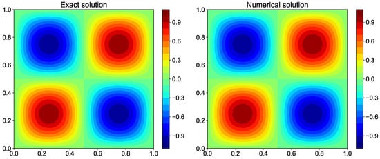
Figure 19. Comparison of exact solution and numerical solution computed using fast sine transform method for the Poisson equation with Dirichlet boundary condition.

Listing 20. Implementation of Julia function for the Poisson solver using fast sine transform (FST) for the domain with Dirichlet boundary condition.

6.2. Iterative Solver

Iterative methods use successive approximations to obtain the most accurate solution to a linear system at every iteration step. These methods start with an initial guess and proceed to generate a sequence of approximations, in which the k-th approximation is derived from the previous ones. There are two main types of iterative methods. Stationary methods that are easy to understand and are simple to implement, but are not very effective. Non-stationary methods which are based on the idea of the sequence of orthogonal vectors. We would like to recommend a text by Barrett et al. [40] which provides a good discussion on the implementation of iterative methods for solving a linear system of equations.

We show only Dirichlet boundary condition implementation for iterative methods. For iterative methods, we stop iterations when the $L_2$ norm of the residual for Equation (83) goes below $1\times {10}^{-10}$. We test the performance of all iterative methods using the method of manufactured solution. The exact field u and the corresponding source term f used for the method of manufactured solution for iterative methods are given below [12]

$$\begin{array}{c}\hfill u(x,y)=(x^2-1)(y^2-1),\end{array}$$

(97)

$$\begin{array}{c}\hfill f(x,y)=-2(2-x^2-y^2).\end{array}$$

(98)

6.2.1. Stationary Methods: Gauss-Seidel

The iterative methods work by splitting the matrix A into

$$A=M-P.$$

(99)

Equation (84) becomes

$$M\mathit{u}=P\mathit{u}+\mathit{b}.$$

(100)

The solution at $(k+1)$ iteration is given by

$$M{\mathit{u}}^{(k+1)}=P{\mathit{u}}^{(k)}+\mathit{b}.$$

(101)

If we take the difference between the above two equations, we get the evolution of error as ${ϵ}^{(k+1)}=M^{-1}P{ϵ}^{(k)}$. For the solution to converge to the exact solution and the error to go to zero, the largest eigenvalue of iteration matrix $M^{-1}P$ should be less than 1. The approximate number of iterations required for the error $ϵ$ to go below some specified tolerance $\delta$ is given by

$$\mathcal{Q}=\frac{\ln (\delta )}{\ln ({\lambda }_1)},$$

(102)

where $\mathcal{Q}$ is the number of iterations and ${\lambda }_1$ is the maximum eigenvalue of iteration matrix $M^{-1}P$. If the convergence tolerance is specified to be $1\times {10}^{-5}$ then the number of iterations for convergence will be $\mathcal{Q}=1146$ and $\mathcal{Q}=23,020$ for ${\lambda }_1=0.99$ and ${\lambda }_1=0.9995$ respectively. Therefore, the maximum eigenvalue of the iteration matrix should be less for faster convergence. When we implement iterative methods, we do not form the matrix M and P. Equation (101) is just the matrix representation of the iterative method. In matrix terms, the Gauss-Seidel method can be expressed as

$$\begin{array}{cc}\hfill M& =D-L,\hfill \end{array}$$

(103)

$$\begin{array}{cc}\hfill {\mathit{u}}^{(k+1)}& ={(D-L)}^{-1}\left(U{\mathit{u}}^{(k)}+b\right),\hfill \end{array}$$

(104)

where D, L and U represent the diagonal, the strictly lower-triangular, and the strictly upper-triangular parts of A, respectively. We do not explicitly construct the matrices D, L, and U, instead we use the update formula based on data vectors (i.e., we obtain a vector once a matrix operates on a vector).

The update formulas for Gauss-Seidel iterations if we iterate from left to right and from bottom to top can be written as

$$\begin{array}{cc}\hfill u_{i,j}^{(k+1)}& =u_{i,j}^{(k)}-\left(\frac{2}{\Delta x^2}+\frac{2}{\Delta y^2}\right)r_{i,j},\hfill \end{array}$$

(105)

where

$$\begin{array}{cc}\hfill r_{i,j}& =f_{i,j}^{(k)}-\frac{u_{i+1,j}^{(k)}-2u_{i,j}^{(k)}+u_{i-1,j}^{(k+1)}}{{\Delta x}^2}-\frac{u_{i,j+1}^{(k)}-2u_{i,j}^{(k)}+u_{i,j-1}^{(k+1)}}{{\Delta y}^2}.\hfill \end{array}$$

(106)

The implementation of the Gauss-Seidel method for Poisson equation in Julia is given in Listing 21. The pseudo algorithm is given by Algorithm 3, where we define an operator $\mathcal{A}$ such that

$$\mathcal{A}{u}_{i,j}=\frac{u_{i+1,j}-2u_{i,j}+u_{i-1,j}}{{\Delta x}^2}+\frac{u_{i,j+1}-2u_{i,j}+u_{i,j-1}}{{\Delta y}^2},$$

(107)

gives same results as matrix-vector multiplication $A\mathit{u}$ for ${(i,j)}^{th}$ grid point. It can be noticed that the matrix M and P are not formed, and the solution is computed using Equation (105) for every point on the grid. Since we are traversing bottom to top and left to right, the updated values on left $(u_{i-1,j})$ and bottom $(u_{i,j-1})$ will be used for updating the solution at ${(i,j)}^{th}$ grid point. This will help in accelerating the convergence compared to the Jacobi method which uses values at the previous iteration step for all its neighboring points.

Figure 20 shows the contour plot for exact and numerical solution for the Gauss-Seidel solver. As seen in Figure 24, the residual reaches ${10}^{-10}$ values after more than 400,000 iterations for Gauss-Seidel method. The maximum eigenvalue of the iteration matrix is large for the Gauss-Seidel method and hence, the rate of convergence is slow. The rate of convergence is higher in the beginning while the high wavenumber errors are still present. Once the high wavenumber errors are resolved, the rate of convergence for low wavenumber errors drops. There are ways to accelerate the convergence such as using successive overrelaxation methods [41]. The residual is computed from Equation (83) as the difference between the source term and the left hand side term computed based on the central-difference scheme. We would like to point out that the residual is different from the discretization error. The discretization error is the difference between numerical and exact solution.

Figure 20. Comparison of exact solution and numerical solution computed using Gauss-Seidel iterative method for the Poisson equation.

Algorithm 3 Gauss-Seidel iterative method
1: Given b	▹ source term
2: $\mathit{u}={\mathit{u}}^{(0)}$	▹ initialize the solution
3: $d=-\left(\frac{2}{{\Delta x}^2}+\frac{2}{{\Delta y}^2}\right)$
4: while tolerance met do
5:  for $i=1$ to $N_x$ do
6:   for $j=1$ to $N_y$ do
7:    $r_{i,j}=b_{i,j}-\mathcal{A}{u}_{i,j}$	▹ compute the residual
8:    $u_{i,j}=u_{i,j}+r_{i,j}/d$	▹ update the solution
9:   end for
10:  end for
11:  check convergence criteria, continue if necessary
12: end while

Listing 21. Implementation of Gauss-Seidel iterative method for Poisson equation in Julia.

6.2.2. Non-Stationary Methods: Conjugate Gradient Algorithm

Non-stationary methods differ from stationary methods in that the iterative matrix changes at every iteration. These methods work by forming a basis of a sequence of matrix powers times the initial residual. The basis is called as the Krylov subspace and mathematically given by ${\mathcal{K}}_n(A,\mathit{b})=\mathrm{span}\{\mathit{b},A\mathit{b},A^2\mathit{b},\cdots ,A^{n-1}\mathit{b}\}$. The approximate solution to the linear system is found by minimizing the residual over the subspace formed. In this paper, we discuss the conjugate gradient method which is one of the most effective methods for symmetric positive definite systems.

The conjugate gradient method proceeds by calculating the vector sequence of successive approximate solution, residual corresponding the approximate solution, and search direction used in updating the solution and residuals. The approximate solution ${\mathit{u}}^{(\mathit{k})}$ is updated at every iteration by a scalar multiple ${\alpha }_k$ of the search direction vector ${\mathit{p}}^{(k)}$:

$${\mathit{u}}^{(k+1)}={\mathit{u}}^{(k)}+{\alpha }_k{\mathit{p}}^{(k)}.$$

(108)

Correspondingly, the residuals ${\mathit{r}}^{(\mathit{k})}$ are updated as

$${\mathit{r}}^{(\mathit{k}+\mathbf{1})}={\mathit{r}}^{(\mathit{k})}-{\alpha }_k{\mathit{q}}^{(k)}\mathrm{where}{\mathit{q}}^{(k)}=\mathcal{A}{\mathit{p}}^{(k)}.$$

(109)

The search directions are then updated using the residuals

$${\mathit{p}}^{(k+1)}={\mathit{r}}^{(k+1)}+{\beta }_k{\mathit{p}}^{(k)},$$

(110)

where the choice ${\beta }_k={\mathit{r}}^{{(k)}^T}{\mathit{r}}^{(k)}/{\mathit{r}}^{{(k-1)}^T}{\mathit{r}}^{(k-1)}$ ensures that ${\mathit{p}}^{(k+1)}$ and ${\mathit{r}}^{(k+1)}$ are orthogonal to all previous $\mathcal{A}{\mathit{p}}^{(k)}$ and ${\mathit{r}}^{(k)}$ respectively. A detailed derivation of the conjugate gradient method can be found in [42]. The complete procedure for the conjugate gradient method is given in Algorithm 4. The implementation of conjugate gradient method in Julia is given in Listing 22.

The comparison of the exact and numerical solution is shown in Figure 21. The residual history for the conjugate gradient method is displayed in Figure 24. It can be seen that the rate of convergence is slower at the start of iterations. As the conjugate gradient algorithm finds the correct direction for residual, the rate of convergence increases. There are several types of iterative methods which are not discussed in this paper and for further reading we refer to a book “Iterative Methods for Sparse Linear Systems” [43].

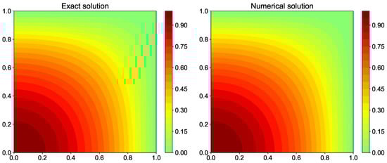
Figure 21. Comparison of exact solution and numerical solution computed using conjugate gradient algorithm for the Poisson equation.

Listing 22. Implementation of conjugate gradient method for Poisson equation in Julia.

Algorithm 4 Conjugate gradient algorithm
1: Given b	▹ Given source term in space, i.e., $\mathit{b}=f(x,y)$ in Equation (82)
2: Given matrix operator $\mathcal{A}$	▹ Given discretization by Equation (107)
3: ${\mathit{u}}^{(0)}=\mathit{b}$	▹ Initialize the solution
4: ${\mathit{r}}^{(0)}=\mathit{b}-\mathcal{A}{\mathit{u}}^{(0)}$	▹ Initialize the residual
5: $p^{(0)}={\mathit{r}}^{(0)}$	▹ Initialize the conjugate
6: $k=0$
7: ${\rho }_0={\mathit{r}}^{{(0)}^T}{\mathit{r}}^{(0)}$
8: while tolerance met (or $k<\mathcal{N}$) do
9:  ${\mathit{q}}^{(k)}=\mathcal{A}{\mathit{p}}^{(k)}$
10:  ${\alpha }_k={\rho }_k/{\mathit{p}}^{{(k)}^T}{\mathit{q}}^{(k)}$
11:  ${\mathit{u}}^{(k+1)}={\mathit{u}}^{(k)}+{\alpha }_k{\mathit{p}}^{(k)}$	▹ Update the solution
12:  ${\mathit{r}}^{(k+1)}={\mathit{r}}^{(k)}-{\alpha }_k{\mathit{q}}^{(k)}$
13:  ${\rho }_{k+1}={\mathit{r}}^{{(k+1)}^T}{\mathit{r}}^{(k+1)}$
14:  ${\beta }_k={\rho }_{k+1}/{\rho }_k$
15:  ${\mathit{p}}^{(k+1)}={\mathit{r}}^{(k+1)}+{\beta }_k{\mathit{p}}^{(k)}$	▹ Update the residual
16:  check convergence; continue if necessary
17:  $k\leftarrow k+1$
18: end while

6.3. Multigrid Framework

We saw in Section 6.2 that the rate of convergence for iterative methods depends upon the iteration matrix $M^{-1}N$. Point iterative methods like Jacobi and Gauss-Seidel methods have large eigenvalue and hence the slow convergence. As the grid becomes finer, the maximum eigenvalue of the iteration matrix becomes close to 1. Therefore, for very high-resolution simulation, these iterative methods are not feasible due to the large computational time required for residuals to go below some specified tolerance.

The multigrid framework is one of the most efficient iterative algorithm to solve the linear system of equations arising due to the discretization of the Poisson equation. The multigrid framework works on the principle that low wavenumber errors on fine grid behave like a high wavenumber error on a coarse grid. In the multigrid framework, we restrict the residuals on the fine grid to the coarser grid. The restricted residual is then relaxed to resolve the low wavenumber errors and the correction to the solution is prolongated back to the fine grid. We can use any of the iterative methods like Jacobi, Gauss-Seidel method for relaxation. The algorithm can be implemented recursively on the hierarchy of grids to get faster convergence.

Let ${\tilde{u}}^{\Delta x}$ denote the approximate solution after applying few steps of iterations of a relaxation method. The fine grid solution will be

$$\begin{array}{c}\hfill \mathcal{A}({\tilde{u}}^{\Delta x}+e^{\Delta x})=b^{\Delta x},\end{array}$$

(111)

$$\begin{array}{c}\hfill \mathcal{A}{e}^{\Delta x}=b^{\Delta x}-\mathcal{A}{\tilde{u}}^{\Delta x},\end{array}$$

(112)

where $e^{\Delta x}$ is the error at fine grid and the operator A is defined in Equation (84) for the Cartesian grid. We define the residual vector $r^{\Delta x}=\mathcal{A}{e}^{\Delta x}$. This residual vector contains mostly low wavenumber errors. The correction at the fine grid is obtained by restricting the residual vector to a coarse grid ($2\Delta x$ grid spacing) and solving an equivalent system to obtain the correction. The equivalent system on a coarse grid can be written as

$${\mathcal{A}}^{2\Delta x}{\tilde{e}}^{2\Delta x}=\mathcal{R}(r^{\Delta x}),$$

(113)

where $A^{2\Delta x}$ is the elliptic operator on coarse grid, and $\mathcal{R}$ is the restriction operator. The discretized form of Equation (113) can be written as

$$\frac{{\tilde{e}}_{i+1,j}^{2\Delta x}-2{\tilde{e}}_{i,j}^{2\Delta x}+{\tilde{e}}_{i-1,j}^{2\Delta x}}{{2\Delta x}^2}+\frac{{\tilde{e}}_{i,j+1}^{2\Delta x}-2{\tilde{e}}_{i,j}^{2\Delta x}+{\tilde{e}}_{i,j-1}^{2\Delta x}}{{2\Delta y}^2}=\mathcal{R}(r_{i,j}^{\Delta x}).$$

(114)

We compute the approximate error at an intermediate grid using some relaxation operation. Once the approximation to ${\tilde{e}}^{2\Delta x}$ is obtained, it is prolongated back to the fine grid using

$${\hat{e}}^{\Delta x}=\mathcal{P}({\tilde{e}}^{2\Delta x}),$$

(115)

where $\mathcal{P}$ is the prolongation operator. The approximate solution at fine grid ${\tilde{u}}^{\Delta x}$ is corrected with ${\hat{e}}^{\Delta x}$. The approximate solution is relaxed for a specific number of iterations and convergence criteria is checked. If the residuals are below specified tolerance we stop or we repeat the steps. The procedure can be easily extended to more number of levels. The illustration of the V-cycle multigrid framework for two levels is shown in Figure 22. In this study, we use two iterations of the Gauss-Seidel method for relaxation at every grid level. The number of iterations can be set to a different number or we can also set the residual tolerance instead of a fixed number of iterations.

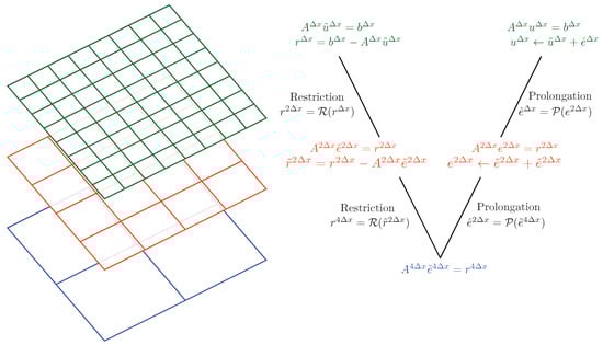
Figure 22. Illustration of multigrid V-cycle framework with three levels between fine and coarse grid. For full multigrid cycle, the coarsest mesh has $2\times 2$ grid resolution and is solved directly.

The residuals corresponding to the fine grid can be projected on to the coarse grid either using full-weighting. The full-weighting restriction operator is given by

$$r_{i,j}^{2\Delta x}=\frac{4r_{2i-1,2j-1}^{\Delta x}+2(r_{2i-1,2j}^{\Delta x}+r_{2i-1,2j-2}^{\Delta x}+r_{2i,2j-1}^{\Delta x}+r_{2i-2,2j-1}^{\Delta x})+r_{2i,2j}^{\Delta x}+r_{2i,2j-2}^{\Delta x}+r_{2i-2,2j}^{\Delta x}+r_{2i-2,2j-2}^{\Delta x}}{16}.$$

(116)

For boundary points, the residuals are directly injected from fine grid to coarse grid. The implementation of restriction operator in Julia is given in Listing 23.

The prolongation operator transfers the error from the coarse grid to the fine grid. We use direct injection for points which are common to both coarse and fine grid and bilinear interpolation for points which are on the fine grid but not on the coarse grid. The prolongation operations are given by below equations

$$\begin{array}{cc}\hfill e_{2i-1,2j-1}^{\Delta x}& =e_{i,j}^{2\Delta x},\hfill \end{array}$$

(117)

$$\begin{array}{cc}\hfill e_{2i-1,2j-1+1}^{\Delta x}& =\frac{e_{i,j}^{2\Delta x}+e_{i,j+1}^{2\Delta x}}{2},\hfill \end{array}$$

(118)

$$\begin{array}{cc}\hfill e_{2i-1+1,2j-1}^{\Delta x}& =\frac{e_{i,j}^{2\Delta x}+e_{i+1,j}^{2\Delta x}}{2},\hfill \end{array}$$

(119)

$$\begin{array}{cc}\hfill e_{2i-1+1,2j-1+1}^{\Delta x}& =\frac{e_{i,j}^{2\Delta x}+e_{i,j+1}^{2\Delta x}+e_{i+1,j}^{2\Delta x}+e_{i+1,j+1}^{2\Delta x}}{2}.\hfill \end{array}$$

(120)

The implementation of prolongation operation in Julia is given in Listing 24.

Listing 23. Implementation of restriction operation in multigrid framework.

Listing 24. Implementation of prolongation operation in multigrid framework.

The relaxation of the solution is done using the Gauss-Seidel method for each grid level as formulated in Section 6.2.1 for a fixed number of iterations. The Julia implementation of relaxation operation is provided in Listing 25. The pseudocode for V-cycle multigrid framework for three levels if provided in Algorithm 5. The implementation of a complete multigrid framework in Julia for two levels is given in Listing 26.

Listing 25. Implementation of relaxation operation (using Gauss-Seidel iterative method) in multigrid framework.

Algorithm 5 V-cycle multigrid framework
1: Given operator $\mathcal{A}$
2: Given v1	▹ number of relaxation operation during restriction
3: Given v2	▹ number of relaxation operation during prolongation
4: Given v3	▹ number of relaxation operation on coarsest grid
5: while tolerance met (or $k<\mathcal{N}$) do
6:  for v1 iterations do
7   $A^{\Delta x}{\tilde{u}}^{\Delta x}=b^{\Delta x}$	▹ relaxation for v1 iterations
8:  end for
9:  check convergence; continue if necessary
10:  $r^{\Delta x}=b^{\Delta x}-A^{\Delta x}{\tilde{u}}^{\Delta x}$	▹ compute residual for fine grid
11:  $r^{2\Delta x}=\mathcal{R}(r^{\Delta x})$	▹ restrict the residual from fine grid to intermediate grid
12:  for v1 iterations do
13:   $A^{2\Delta x}{\tilde{e}}^{2\Delta x}=r^{2\Delta x}$	▹ relaxation of error for v1 iterations
14:  end for
15:  ${\tilde{r}}^{2\Delta x}=r^{2\Delta x}-A^{2\Delta x}{\tilde{e}}^{2\Delta x}$	▹ compute residual using error at intermediate grid
16:  $r^{4\Delta x}=\mathcal{R}({\tilde{r}}^{2\Delta x})$	▹ restrict the residual for error to coarsest grid
17:  for v3 iterations do	▹ can be solved directly instead of v3 iterations
18:   $A^{4\Delta x}{\tilde{e}}^{4\Delta x}=r^{4\Delta x}$	▹ relaxation of error for v3 iterations
19:  end for
20:  ${\hat{e}}^{2\Delta x}=\mathcal{P}({\tilde{e}}^{4\Delta x})$	▹ prolongate error from coarsest grid to intermediate level
21:  $e^{2\Delta x}\leftarrow {\tilde{e}}^{2\Delta x}+{\hat{e}}^{2\Delta x}$	▹ add correction to the error at intermediate grid
22:  for v2 iterations do
23:   $A^{2\Delta x}{e}^{2\Delta x}=r^{2\Delta x}$	▹ relaxation of error for v2 iterations
24:  end for
25:  ${\hat{e}}^{\Delta x}=\mathcal{P}(e^{2\Delta x})$	▹ prolongate error from intermediate grid to coarse grid
26:  $u^{\Delta x}\leftarrow {\tilde{u}}^{\Delta x}+{\hat{e}}^{\Delta x}$	▹ add correction to the solution at fine level
27:  for v2 iterations do
28:   $A^{\Delta x}{u}^{\Delta x}=b^{\Delta x}$	▹ relaxation of solution for v2 iterations
29:  end for
30: end while

Listing 26. Implementation of multigrid framework in Julia with two levels in V-cycle.

Figure 23 displays the comparison of exact solution and numerical solution for full V-cycle multigrid framework. We use 512 × 512 grid resolution and hence we use nine levels from fine mesh to coarsest mesh. When the coarsest mesh has 2 × 2 grid resolution (i.e., since boundaries are set zero, only one grid point value is unknown and that can be solved algebraically), then it is usually referred to as the full multigrid framework. Figure 24 shows that the residual drops below tolerance in just nine iterations. This does not consist of a number of iterations for relaxation operations done for each intermediate grid levels. Although we report the outer iteration counter for multigrid results, we highlight that the workload in multigrid is more than the outer iteration counts. Equation (121) gives the total iteration count for a typical V-cycle multigrid method:

$$\mathrm{V}-\mathrm{cycle}\mathrm{multigrid}\cos \mathrm{t}=V\left((v_1+v_2)\sum _{d=0}^{L-2}\frac{1}{2^d}+v_3\frac{1}{2^{L-1}}\right),$$

(121)

where V is the outer iteration count, $v_1$ and $v_2$ are the number of iterations during prolongation and restriction, $v_3$ is the number of iterations for coarsest grid, and L is total number of levels in full multigrid cycle. In a typical application, the values of $v_1=2$, $v_2=2$, and $v_3=1$ can work effectively (i.e., a higher value of $v_3$ can be used if the coarsest resolution is larger than $2\times 2$ and intended to be solved by the same relaxation method). Table 2 provides the comparison of different iterative solvers for the Poisson equation.

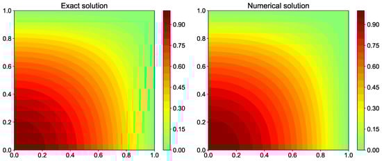
Figure 23. Comparison of exact solution and numerical solution computed using multigrid framework for the Poisson equation.

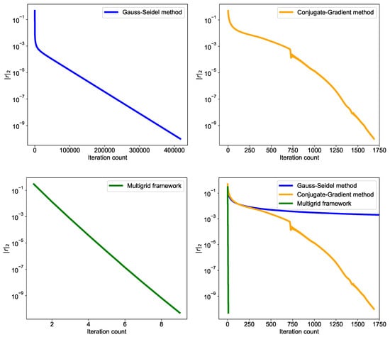
Figure 24. Residual history comparison for different iterative methods for Poisson equation with Dirichlet boundary condition. The stopping criteria for all iterative methods is that the residual should reduce below ${10}^{-10}$. The grid resolution for all cases is $N_x=512$ and $N_y=512$.

Table 2. Comparison of different iterative methods in terms of iteration count, residual and CPU time for solving the Poisson equation on a resolution of $N_x=512$ and $N_y=512$.

Iterative Solver	Iteration Count	Residual	CPU Time (s)
Gauss-Seidel	416,946	$9.99\times {10}^{-11}$	1662.08
Conjugate-Gradient	1687	$9.88\times {10}^{-11}$	4.30
V-cycle Multigrid	9	$5.04\times {10}^{-11}$	0.55

7. Incompressible Two-Dimensional Navier-Stokes Equation

The Navier-Stokes equations for incompressible flow can be written as

$$\begin{array}{cc}\hfill \mathsf{\nabla }·\mathbf{u}& =0,\hfill \end{array}$$

(122)

$$\begin{array}{cc}\hfill \frac{\partial \mathbf{u}}{\partial t}+\mathbf{u}·\mathsf{\nabla }\mathbf{u}& =-\frac{1}{\rho }\mathsf{\nabla }p+\nu {\mathsf{\nabla }}^2\mathbf{u},\hfill \end{array}$$

(123)

where $\mathbf{u}=[\mathrm{u},\mathrm{v}]$ is the velocity vector, t is the time, $\rho$ is the density, p is pressure, and $\nu$ is the kinematic viscosity. By taking curl of Equation (123) and using $\mathsf{\nabla }\times \mathbf{u}=\omega$, we can derive the vorticity equation

$$\mathsf{\nabla }\times \frac{\partial \mathbf{u}}{\partial t}+\mathsf{\nabla }\times (\mathbf{u}·\mathsf{\nabla }\mathbf{u})=-\mathsf{\nabla }\times \left(\frac{1}{\rho }\mathsf{\nabla }p\right)+\mathsf{\nabla }\times \nu {\mathsf{\nabla }}^2\mathbf{u}.$$

(124)

The first term on the left side and last term on the right side becomes

$$\mathsf{\nabla }\times \frac{\partial \mathbf{u}}{\partial t}=\frac{\partial \omega }{\partial t};\mathsf{\nabla }\times \nu {\mathsf{\nabla }}^2\mathbf{u}=\nu {\mathsf{\nabla }}^2\omega .$$

(125)

Applying the identity $\mathsf{\nabla }\times \mathsf{\nabla }f=0$ for any scalar function f, the pressure term vanishes for the incompressible flow since the density is constant

$$\mathsf{\nabla }\times \mathsf{\nabla }\left(\frac{p}{\rho }\right)=0.$$

(126)

The second term in Equation (123) can be writtern as

$$\mathbf{u}·\mathsf{\nabla }\mathbf{u}=\frac{1}{2}\mathsf{\nabla }(\mathbf{u}·\mathbf{u})-\mathbf{u}\times (\mathsf{\nabla }\times \mathbf{u})=\mathsf{\nabla }\left(\frac{{\mathbf{u}}^2}{2}\right)-\mathbf{u}\times \omega \mathrm{where}{\mathbf{u}}^2=\mathbf{u}·\mathbf{u}.$$

(127)

The second term in Equation (124) becomes

$$\begin{array}{cc}\hfill \mathsf{\nabla }\times (\mathbf{u}·\mathsf{\nabla }\mathbf{u})& =\mathsf{\nabla }\times \mathsf{\nabla }\left(\frac{{\mathbf{u}}^2}{2}\right)-\mathsf{\nabla }\times \mathbf{u}\times \omega =\mathsf{\nabla }\times (\omega \times \mathbf{u})\hfill \\ \hfill & =(\mathbf{u}·\mathsf{\nabla })\omega -\underset{(\mathrm{vortex} \mathrm{stretching})}{\underbrace{(\omega ·\mathsf{\nabla })\mathbf{u}}}+\underset{\mathsf{\nabla }·\mathbf{u}=0(\mathrm{incompressible}\mathrm{flow})}{\underbrace{\omega (\mathsf{\nabla }·\mathbf{u})}}+\underset{\mathsf{\nabla }·(\mathsf{\nabla }\times \mathbf{u})=0}{\underset{}{\underbrace{\mathbf{u}(\mathsf{\nabla }·\omega )}}},\hfill \end{array}$$

(128)

and the vortex stretching term vanishes in two-dimensional flows (i.e., ${\omega }_x=0$, ${\omega }_y=0$, ${\omega }_z=\omega$)

$$\begin{array}{cc}\hfill (\omega ·\mathsf{\nabla })\mathbf{u}& =\left(\underset{0}{\underbrace{{\omega }_x}}\frac{\partial }{\partial x}+\underset{0}{\underbrace{{\omega }_y}}\frac{\partial }{\partial y}+{\omega }_z\underset{0}{\underbrace{\frac{\partial }{\partial z}}}\right)=0.\hfill \end{array}$$

(129)

We can further use below relations for two-dimensional flows

$$\begin{array}{cc}\hfill (\mathbf{u}·\mathsf{\nabla })\omega & =\mathrm{u}\frac{\partial \omega }{\partial x}+\mathrm{v}\frac{\partial \omega }{\partial y},\hfill \end{array}$$

(130)

and introducing a streamfunction with the following definitions:

$$\begin{array}{c}\hfill \mathrm{u}=\frac{\partial \psi }{\partial y},\mathrm{and}\mathrm{v}=-\frac{\partial \psi }{\partial x},\end{array}$$

(131)

then the advection term becomes (i.e., sometimes called nonlinear Jacobian)

$$\begin{array}{cc}\hfill (\mathbf{u}·\mathsf{\nabla })\omega & =\frac{\partial \psi }{\partial y}\frac{\partial \omega }{\partial x}-\frac{\partial \psi }{\partial x}\frac{\partial \omega }{\partial y}.\hfill \end{array}$$

(132)

The vorticity equation for two-dimensional incompressible flow becomes

$$\frac{\partial \omega }{\partial t}+\frac{\partial \psi }{\partial y}\frac{\partial \omega }{\partial x}-\frac{\partial \psi }{\partial x}\frac{\partial \omega }{\partial y}=\nu \left(\frac{{\partial }^2\omega }{\partial x^2}+\frac{{\partial }^2\omega }{\partial y^2}\right).$$

(133)

The kinematic relationship between streamfunction and vorticity is given by a Poisson equation

$$\frac{{\partial }^2\psi }{\partial x^2}+\frac{{\partial }^2\psi }{\partial y^2}=-\omega .$$

(134)

The vorticity-streamfunction formulation has several advantages over solving Equations (122) and (123). It eliminates the pressure term from the momentum equation and hence, there is no odd-even coupling between the pressure and velocity. We can use vorticity-streamfunction formulation directly on the collocated grid instead of using staggered grid. The number of equations to be solved in the vorticity-streamfunction formulation is also less than primitive variable formulation as it satisfies the divergence-free condition.

We use third-order Runge-Kutta numerical scheme (as discussed in Section 2.2) for the time integration. The right hand side terms in Equation (133) is discretized using the second-order central difference scheme similar to the diffusion term in heat equation (refer to Section 2.1). The nonlinear terms in Equation (133) is defined as the Jacobian

$$J(\omega ,\psi )=\frac{\partial \psi }{\partial y}\frac{\partial \omega }{\partial x}-\frac{\partial \psi }{\partial x}\frac{\partial \omega }{\partial y}.$$

(135)

We can use any discretization method like explicit finite difference scheme (refer to Section 2.1) or compact finite difference scheme (refer to Section 2.4) for each term in Equation (135). Here, we use a numerical scheme introduced by Arakawa [44] for the discretization of Equation (135). This numerical scheme has conservation of energy, enstrophy and skew symmetry property and avoids computational instabilities arising from nonlinear interactions. The second-order Arakawa scheme for Equation (135) is given below

$$J(\omega ,\psi )=\frac{J_1(\omega ,\psi )+J_2(\omega ,\psi )+J_3(\omega ,\psi )}{3},$$

(136)

where the discrete parts of the Jacobian are

$$\begin{array}{cc}\hfill & \begin{array}{cc}\hfill J_1(\omega ,\psi )& =\frac{({\omega }_{i+1,j}-{\omega }_{i-1,j})({\psi }_{i,j+1}-{\psi }_{i,j-1})-({\omega }_{i,j+1}-{\omega }_{i,j-1})({\psi }_{i+1,j}-{\psi }_{i-1,j})}{4\Delta x\Delta y},\hfill \end{array}\hfill \end{array}$$

(137)

$$\begin{array}{cc}\hfill & \begin{array}{c}\hfill J_2(\omega ,\psi )=\frac{1}{4\Delta x\Delta y}[{\omega }_{i+1,j}({\psi }_{i+1,j+1}-{\psi }_{i+1,j-1})-{\omega }_{i-1,j}({\psi }_{i-1,j+1}-{\psi }_{i-1,j-1})\\ \hfill -{\omega }_{i,j+1}({\psi }_{i+1,j+1}-{\psi }_{i-1,j+1})+{\omega }_{i,j-1}({\psi }_{i+1,j-1}-{\psi }_{i-1,j-1})],\end{array}\hfill \end{array}$$

(138)

$$\begin{array}{cc}\hfill & \begin{array}{c}\hfill J_3(\omega ,\psi )=\frac{1}{4\Delta x\Delta y}[{\omega }_{i+1,j+1}({\psi }_{i,j+1}-{\psi }_{i+1,j})-{\omega }_{i-1,j-1}({\psi }_{i-1,j}-{\psi }_{i,j-1})\\ \hfill -{\omega }_{i-1,j+1}({\psi }_{i,j+1}-{\psi }_{i-1,j})+{\omega }_{i+1,j-1}({\psi }_{i+1,j}-{\psi }_{i,j-1})].\end{array}\hfill \end{array}$$

(139)

7.1. Lid-Driven Cavity Problem

We test our two-dimensional Navier-Stokes solver using the lid-driven cavity benchmark problem for viscous incompressible flow [45]. The problem deals with a square cavity consisting of three rigid walls with no-slip conditions and a lid moving with a tangential unit velocity. The density of the fluid is taken to be unity. Therefore, we get $\nu =1/\mathrm{Re}$, where Re is the Reynolds number of flow. The vorticity equation for lid-driven cavity problem can be written as

$$\frac{\partial \omega }{\partial t}=-\left(\frac{\partial \psi }{\partial y}\frac{\partial \omega }{\partial x}-\frac{\partial \psi }{\partial x}\frac{\partial \omega }{\partial y}\right)+\frac{1}{\mathrm{Re}}\left(\frac{{\partial }^2\omega }{\partial x^2}+\frac{{\partial }^2\omega }{\partial y^2}\right).$$

(140)

The computational domain is square in shape with $(x,y)\in [0,1]\times [0,1]$. We divide the computational domain into $64\times 64$ grid resolution. All the walls have Dirichlet boundary conditions. The time integration implementation in Julia for two-dimensional Navier-Stokes solver is similar to Listing 2. We perform time integration from time $t=0$ to $t=10$ to make sure that steady state is reached and the residual reaches below ${10}^{-6}$. The residual is defined as the $L_2$ norm of the difference between two consecutive solutions. At each step of the Runge-Kutta numerical scheme, we also update the boundary condition for vorticity (i.e., further details can be found in [46]) and solve Equation (134) to update streamfunction. Any of the Poisson solvers mentioned in Section 6 can be used to solve this equation. We use fast sine transform Poisson solver discussed in Section 6.1.2 to get streamfunction from vorticity field as we have Dirichlet boundary conditions for all four walls. The implementation of FST Poisson solver in Julia is given in Listing 20. The functions to compute the right-hand side term for Runge-Kutta numerical scheme and to update boundary conditions are given in Listings 27 and 28 respectively. Figure 25 shows the vorticity and streamfunction field for the lid driven cavity problem.

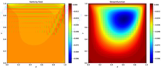
Figure 25. Vorticity field and streamfunction field for the lid-driven cavity benchmark problem.

Listing 27. Computation of right-hand side term in Equation (140) in Julia for two-dimensional incompressible Navier-Stokes equations.

Listing 28. Boundary condition update function in Julia for the lid-driven cavity problem.

7.2. Vortex-Merger Problem

We demonstrate the two-dimensional Navier-Stokes solver for the domain with periodic boundary condition using vortex-merger problem. The merging process occurs when two vortices of the same sign with parallel axes are within a certain critical distance from each other. The two vortices merge to form a single vortex. It is a two-dimensional process and is one of the fundamental processes of fluid motion and it plays a key role in a variety of simulations, such as decaying two-dimensional turbulence, three-dimensional turbulence, and mixing layers [47,48,49]. This phenomenon also occurs in other fields such as astrophysics, meteorology, and geophysics [50].

We use the Cartesian computational domain $(x,y)\in [0,2\pi ]\times [0,2\pi ]$ and divide it into $128\times 128$ grid resolution. The vorticity equation for the vortex-merger problem is same as the lid-driven cavity problem and is given in Equation (140). We use $\mathrm{Re}=2000$ and integrate the solution from time $t=0$ to $t=20$ with $\Delta t=0.01$. We use third-order Runge-Kutta method for time integration similar to the lid-driven cavity problem. The Julia function to compute the right hand side term of vorticity equation is the same as the lid-driven cavity problem and is given in Listing 27. The Julia function to assign the initial condition for vortex-merger problem is detailed in Listing 29.

Listing 29. Initial condition assignment function in Julia for vortex-merger problem.

The vortex-merger problem has the periodic domain and hence we use fast Fourier transform (FFT) Poisson solver discussed in Section 6.1.1 to get the streamfunction from vorticity field at every time step. The Julia function for FFT Poisson solver is outlined in Listing 18. The evolution of the merging process for two vortices into a single vortex is displayed in Figure 26. If we let the simulation run for some more time, we will see a single vortex getting formed.

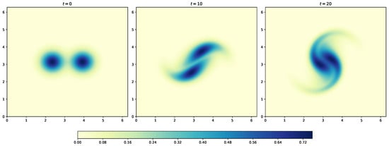
Figure 26. Evolution of the vorticity field at three time steps during the co-rotating vortex interaction. The solution is computed using second-order explicit solver.

We compare the computational time required for two-dimensional incompressible Navier-Stokes solver in Julia with Python code. We use two versions of Python code. In the first version, we use for loop similar to the way we write Julia code. The Python code for computing the right hand side term using Arakawa numerical scheme is given in Listing 30. The other version is the vectorized version which speeds up the code without using any loops and is given in Listing 31. In vectorization, several operations such as multiplication, addition, division are performed over a vector at the same time. From Table 3, we can easily see the benefit of Julia over Python for computationally intensive problems like the ones encountered in CFD applications.

Table 3. Comparison of CPU time for Julia and Python version of Navier-Stokes solver for grid resolution $N_x=128$ and $N_y=128$. We note that the codes are written mostly for the pedagogical purpose and the CPU time may not be the optimal time that can be achieved for each of the programming languages.

Programming Language	CPU Time (s)
Julia	5.97
Python (nonvectorized)	1271.55
Python (vectorized)	18.46

Listing 30. Computation of right hand side function in Python without vectorization.

Listing 31. Computation of right hand side function in Python with vectorization.

8. Hybrid Arakawa-Spectral Solver

In this section, instead of using a fully explicit method in time for solving 2D incompressible Navier-Stokes equation, we show how to design hybrid explicit and implicit scheme. The nonlinear Jacobian term in vorticity Equation (133) is treated explicitly using third-order Runge-Kutta scheme, and we treat the viscous term implicitly using the Crank-Nicolson scheme. This type of hybrid approach is useful when we design solvers for wall-bounded flows, where we cluster the grid in the boundary layer. For wall-bounded flows, we use dense mesh with a smaller grid size in the boundary layer region to capture the boundary layer flow correctly. First, we can re-write Equation (133) with nonlinear Jacobian term on the right hand side

$$\frac{\partial \omega }{\partial t}=-J(\omega ,\psi )+\nu {\mathsf{\nabla }}^2\omega .$$

(141)

The hybrid third-order Runge-Kutta/Crank-Nicolson scheme can be written as [51]

$$\begin{array}{cc}\hfill {\omega }^{(1)}& ={\omega }^{(n)}+{\gamma }_1\Delta t(-J^{(n)})+{\rho }_1\Delta t(-J^{(n-1)(2)})+\frac{{\alpha }_1\Delta t\nu }{2}{\mathsf{\nabla }}^2({\omega }^{(1)}+{\omega }^{(n)}),\hfill \end{array}$$

(142)

$$\begin{array}{cc}\hfill {\omega }^{(2)}& ={\omega }^{(1)}+{\gamma }_2\Delta t(-J^{(1)})+{\rho }_2\Delta t(-J^{(n)})+\frac{{\alpha }_2\Delta t\nu }{2}{\mathsf{\nabla }}^2({\omega }^{(1)}+{\omega }^{(2)}),\hfill \end{array}$$

(143)

$$\begin{array}{cc}\hfill {\omega }^{(n+1)}& ={\omega }^{(2)}+{\gamma }_3\Delta t(-J^{(2)})+{\rho }_3\Delta t(-J^{(1)})+\frac{{\alpha }_3\Delta t\nu }{2}{\mathsf{\nabla }}^2({\omega }^{(n+1)}+{\omega }^{(2)}),\hfill \end{array}$$

(144)

where the term $-J^{(n-1)(2)}$ is the nonlinear Jacobian term at the second-step of previous time step at $(n-1)$. We can choose coefficients in Equations (142)–(144) in such a way that ${\rho }_1$ vanishes and we do not have to store the solution at second-step of the previous time step. These coefficients are

$$\begin{array}{cc}\hfill {\alpha }_1& =\frac{8}{15},{\alpha }_2=\frac{2}{15},{\alpha }_3=\frac{1}{3},\hfill \end{array}$$

(145)

$$\begin{array}{cc}\hfill {\gamma }_1& =\frac{8}{15},{\gamma }_2=\frac{5}{12},{\gamma }_3=\frac{3}{4},\hfill \end{array}$$

(146)

$$\begin{array}{cc}\hfill {\rho }_1& =0,{\rho }_2=-\frac{17}{60},{\rho }_2=-\frac{5}{12}.\hfill \end{array}$$

(147)

Besides, to use a hybrid scheme for time, we also design a hybrid finite difference and spectral scheme. We use Arakawa finite difference scheme for the nonlinear Jacobian term and spectral scheme for linear viscous terms. In Fourier space, Equations (142)–(144) can be written as

$$\begin{array}{cc}\hfill {\tilde{\omega }}^{(1)}& ={\tilde{\omega }}^{(n)}+{\gamma }_1\Delta t(-{\tilde{J}}^{(n)})+{\rho }_1\Delta t(-{\tilde{J}}^{(n-1)(2)})+\frac{{\alpha }_1\Delta t\nu }{2}(-k^2)({\tilde{\omega }}^{(1)}+{\tilde{\omega }}^{(n)}),\hfill \end{array}$$

(148)

$$\begin{array}{cc}\hfill {\tilde{\omega }}^{(2)}& ={\tilde{\omega }}^{(1)}+{\gamma }_2\Delta t(-{\tilde{J}}^{(1)})+{\rho }_2\Delta t(-{\tilde{J}}^{(n)})+\frac{{\alpha }_2\Delta t\nu }{2}(-k^2)({\tilde{\omega }}^{(1)}+{\tilde{\omega }}^{(2)}),\hfill \end{array}$$

(149)

$$\begin{array}{cc}\hfill {\tilde{\omega }}^{(n+1)}& ={\tilde{\omega }}^{(2)}+{\gamma }_3\Delta t(-{\tilde{J}}^{(2)})+{\rho }_3\Delta t(-{\tilde{J}}^{(1)})+\frac{{\alpha }_3\Delta t\nu }{2}(-k^2)({\tilde{\omega }}^{(n+1)}+{\tilde{\omega }}^{(2)}),\hfill \end{array}$$

(150)

where $k^2=m^2+n^2$. Here, m and n are wavenumber in x and y directions, respectively. Rearranging above equations, we get

$$\begin{array}{cc}\hfill {\tilde{\omega }}^{(1)}& =\frac{1-\frac{{\alpha }_1\Delta t\nu k^2}{2}}{1+\frac{{\alpha }_1\Delta t\nu k^2}{2}}{\tilde{\omega }}^{(n)}+\frac{{\gamma }_1\Delta t}{1+\frac{{\alpha }_1\Delta t\nu k^2}{2}}(-{\tilde{J}}^{(n)}),\hfill \end{array}$$

(151)

$$\begin{array}{cc}\hfill {\tilde{\omega }}^{(2)}& =\frac{1-\frac{{\alpha }_2\Delta t\nu k^2}{2}}{1+\frac{{\alpha }_2\Delta t\nu k^2}{2}}{\tilde{\omega }}^{(1)}+\frac{{\gamma }_2\Delta t(-{\tilde{J}}^{(1)})+{\rho }_2\Delta t(-{\tilde{J}}^{(n)})}{1+\frac{{\alpha }_2\Delta t\nu k^2}{2}},\hfill \end{array}$$

(152)

$$\begin{array}{cc}\hfill {\tilde{\omega }}^{(n+1)}& =\frac{1-\frac{{\alpha }_3\Delta t\nu k^2}{2}}{1+\frac{{\alpha }_3\Delta t\nu k^2}{2}}{\tilde{\omega }}^{(2)}+\frac{{\gamma }_3\Delta t(-{\tilde{J}}^{(2)})+{\rho }_3\Delta t(-{\tilde{J}}^{(1)})}{1+\frac{{\alpha }_3\Delta t\nu k^2}{2}}.\hfill \end{array}$$

(153)

We use Arakawa finite difference scheme described in Section 7 to compute the Jacobian term in physical space. The streamfunction is computed from the vorticity field using a spectral method. Once the Jacobian term is available in physical space we convert it to Fourier space using FFT. The relationship between vorticity and streamfunction is Fourier space can be written as

$$\tilde{\psi }=\frac{\tilde{\omega }}{k^2}.$$

(154)

The time integration using hybrid third-order Runge-Kutta/ Crank-Nicolson scheme in Julia is listed in Listing 32. The Julia implementation to compute the nonlinear Jacobian term for the Arakawa-spectral solver is given in Listing 33.

Listing 32. Julia implementation of hybrid third-order Runge-Kutta/ Crank-Nicolson scheme for 2D incompressible Navier-Stokes equation with Arakawa-spectral finite difference scheme.

Listing 33. Julia implementation of computing the nonlinear Jacobian term in physical space and converting it to Fourier space.

We validate our hybrid Arakawa-spectral solver for vortex-merger problem. Figure 27 shows the evolution of two point vortices merging into a single vortex computed using hybridized finite difference and spectral methodology. In the next section, we will eliminate finite difference and present a pseudo-spectral methodology.

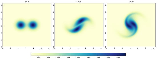
Figure 27. Evolution of the vorticity field at three time steps during the co-rotating vortex interaction. The solution is computed using hybrid Arakawa-spectral solver.

9. Pseudo-Spectral Solver

In Section 8, we computed the Jacobian term using finite difference Arakawa scheme. We can also compute this term using a spectral method to develop the pseudo-spectral solver. The main motivation for the spectral solver is a unique advantage of both accuracy and efficiency considerations in simple geometries. It reduces a PDE problem to a set of ODEs without introducing a numerical discretization error. Furthermore, the code implementation will be much simpler due to the availability of FFT libraries. We refer to a paper by Mortensen and Langtangen [52] for further discussion of high performance pseudo-spectral solver implementation of 3D Navier-Stokes equations. We use the hybrid explicit and implicit Crank-Nicolson scheme for time integration similar to the previous section. The only difference is the computation of the Jacobian term. The Jacobian term involves the first derivative term and can be calculated easily using a spectral method. The first derivative of Equation (88) in x and y direction is calculated as

$$\begin{array}{cc}\hfill \frac{\partial }{\partial x}{u}_{i,j}& =\frac{1}{N_x}\frac{1}{N_y}\sum _{m=-N_x/2}^{N_x/2-1}\sum _{n=-N_y/2}^{N_y/2-1}\left(\iota m\right){\tilde{u}}_{m,n}{e}^{\iota 2\pi \left(\frac{mi}{N_x}+\frac{nj}{N_y}\right)},\hfill \end{array}$$

(155)

$$\begin{array}{cc}\hfill \frac{\partial }{\partial y}{u}_{i,j}& =\frac{1}{N_x}\frac{1}{N_y}\sum _{m=-N_x/2}^{N_x/2-1}\sum _{n=-N_y/2}^{N_y/2-1}\left(\iota n\right){\tilde{u}}_{m,n}{e}^{\iota 2\pi \left(\frac{mi}{N_x}+\frac{nj}{N_y}\right)}.\hfill \end{array}$$

(156)

The Jacobian term in the Fourier space can be computed as

$${\tilde{J}}_{m,n}=(\iota n\tilde{\psi })⊛(\iota m\tilde{\omega })-(\iota m\tilde{\psi })⊛(\iota n\tilde{\omega }),$$

(157)

where ⊛ is the convolution operation. Using Equation (154), we get

$${\tilde{J}}_{m,n}=\left(\iota n\frac{\tilde{\omega }}{k^2}\right)⊛(\iota m\tilde{\omega })-\left(\iota m\frac{\tilde{\omega }}{k^2}\right)⊛(\iota n\tilde{\omega }).$$

(158)

The convolution operation is performed in physical space and then converted to physical space. The pseudo-code for calculating the Jacobian term is given as

$${\tilde{J}}_{m,n}=\mathrm{fft}[\underset{\frac{\partial \psi }{\partial y}}{\underbrace{\mathrm{ifft}(\iota n\frac{\tilde{\omega }}{k^2})}}⊛\underset{\frac{\partial \omega }{\partial x}}{\underbrace{\mathrm{ifft}(\iota m\tilde{\omega })}}-\underset{\frac{\partial \psi }{\partial x}}{\underbrace{\mathrm{ifft}(\iota m\frac{\tilde{\omega }}{k^2})}}⊛\underset{\frac{\partial \omega }{\partial y}}{\underbrace{\mathrm{ifft}(\iota n\tilde{\omega })}}].$$

(159)

We can observe that the Jacobian term involves the product of two functions. When we evaluate the product of two functions using Fourier transform, aliasing errors appear in the computation [12]. Aliasing errors refers to the misrepresentation of wavenumbers when the function is mapped onto a grid with not enough grid points. One way to reduce aliasing errors is to use 3/2-rule. In this method, the original grid is refined by a factor $\mathit{M}=3/2N$ in each direction. The additional grid points are assigned zero value and this is also referred to as zero-padding. For example, if we are using spatial resolution of $N_x=128$ and $N_y=128$ in x and y direction, the Jacobian term will be evaluated on grid with $N_x=192$ and $N_y=192$ (i.e., a data set consisted of ${192}^2$ points is used in the inverse and forward FFT calls in Equation (159)). The main code for the pseudo-spectral solver is the same as the hybrid solver discussed in Section 8 except for the Jacobian function. The implementation of Jacobian calculation with 3/2 padding is given in Listing 34.

Listing 34. Julia implementation of computing the nonlinear Jacobian term in Fourier space with 3/2 padding rule.

We compare the performance of pseudo-spectral solver for two-dimensional incompressible flow problems written in Julia with the vectorized version of Python code. The FFT operations in Julia are performed using the FFTW package. We use two different packages for FFT operations in Python: Numpy library and pyFFTW package. We measure the CPU time for two grid resolutions: $N_x=N_y=128$ and $N_x=N_y=256$. We test two codes at $Re=1000$ with $\Delta t=0.01$ from time $t=0$ to $t=20$. The CPU time for two grid resolutions for two versions of code is provided in Table 4. It can be seen that the computational time for Julia is slightly better than Python code with the Numpy library for performing FFT operations. The pyFFTW package uses FFTW which is a very fast C library. The computational time required by vectorized Python code with pyFFTW package is better than the Julia code. This might be due to the effective interface between the FFTW library and pyFFTW package. Therefore, each programming language has some benefits over others. However, the goal of this study is not to optimize the code or find the best scientific programming language but is to present how can one implement CFD codes.

Table 4. Comparison of CPU time for Julia and Python version of pseudo-spectral solver at two grid resolutions. We highlight that the codes are not written for optimization purpose and the CPU time may not be the optimal time that can be achieved for each of the programming languages.

Programming Language	CPU Time (s)
	${\mathit{N}}_{\mathit{x}},{\mathit{N}}_{\mathit{y}}=\mathbf{128}$	${\mathit{N}}_{\mathit{x}},{\mathit{N}}_{\mathit{y}}=\mathbf{256}$
Julia	31.25	163.63
Python (Numpy)	37.05	181.07
Python (pyFFTW)	21.76	105.81

Another common technique to reduce aliasing error which is widely used in practice is to use 2/3-rule. In this technique we retain the data on 2/3 of the grid is retained, while the remaining data is assigned with zero value. For example, if we are using a spatial resolution of $N_x=128$ and $N_y=128$ (i.e., $-64\le k_x\le 64$ and $-64\le k_y\le 64$), we will retain the Fourier coefficients corresponding to (−42 to 42) and remaining Fourier coefficients are set zero. One of the advantages of using this method is that it is computationally efficient since the Fourier transform of the matrix having size as the power of 2 is more efficient than the matrix which has dimension non-powers of 2. If we use $2/3$-rule it is equivalent to performing calculation on $N_x=85$ and $N_y=85$ grid. However, a data set consisted of ${128}^2$ points is used in the inverse and forward FFT calls in Equation (159). The implementation of Jacobian calculation with $2/3$ padding is given in Listing 35. Before we close this section, we would like to note that there is no significant aliasing error in the example presented in this section. Therefore, one might get similar results without performing any padding (1/1 rule).

Listing 35. Julia implementation of computing the nonlinear Jacobian term in Fourier space with 2/3 padding rule.

10. Concluding Remarks

The easy syntax and fast performance of Julia programming language make it one of the best candidates for engineering students, especially from a non-computer science background to develop codes to solve problems they are working on. We use Julia language as a tool to solve basic fluid flow problems which can be included in graduate-level CFD coursework. We follow a similar pattern as teaching a class, starting from basics and then building upon it to solve more advanced problems. We provide small pieces of code developed for simple fundamental problems in CFD. These pieces of codes can be used as a starting point and one can go about adding more features to solve complex problems. We make all codes, plotting scripts available online and open to everyone. All the codes are made available online to everyone on Github (https://github.com/surajp92/CFD_Julia).

We explain fundamental concepts of finite difference discretization, explicit methods, implicit methods using one-dimensional heat equation in Section 2. We also outline the procedure to develop a compact finite difference scheme which gives higher-order accuracy with smaller stencil size. We present a multi-step Runge-Kutta method which has higher temporal accuracy than standard single step finite difference method. We illustrate numerical methods for hyperbolic conservation laws using the inviscid Burgers equation as the prototype example in Section 3. We demonstrate two shock-capturing methods: WENO-5 and CRWENO-5 methods for Dirichlet and periodic boundary conditions. Students can learn about WENO reconstruction and boundary points treatment which is also applicable to other problems.

We show an implementation of the finite difference method for the inviscid Burgers equation in its conservative form in Section 4. Students will get insight into a finite volume method implementation through this example. We present two approaches for computing fluxes at the interface using the flux splitting method and using Riemann solver. We use Riemann solver based on simple Rusanov scheme. Students can easily implement other methods by changing the function for Rusanov scheme. We also develop one-dimensional Euler solver and validate it for the Sod shock tube problem in Section 5. We borrow functions from heat equation codes, such as Runge-Kutta code for time integration. We use WENO-5 code developed for the inviscid Burgers equation for solving Euler equations. This will give students an understanding of how coding blocks developed for simple problems can be integrated to solve more challenging problems.

We illustrate different methods to solve elliptic equations using Poisson equation as an example in Section 6. We describe both direct methods and iterative methods to solve the Poisson equation. The direct solvers explained in this study are based on the Fourier transform. We demonstrate an implementation of FFT and FST for developing a Poisson solver for periodic and Dirichlet boundary condition respectively. We provide an overview of two iterative methods: Gauss-Seidel method and conjugate gradient method for the Poisson equation. Furthermore, we demonstrate the implementation of the V-cycle multigrid framework for the Poisson equation. A multigrid framework is a powerful tool for CFD simulations as it scales linearly, i.e., it has $O(N)$ computational complexity.

We describe two-dimensional incompressible Navier-Stokes solver in Section 7 and validate it for two examples: lid-driven cavity problem and vortex-merger problem. We use streamfunction-vorticity formulation to develop the solver. This eliminates the pressure term in the momentum equation and we can use the collocated grid arrangement instead of the staggered grid arrangement. We use Arakawa numerical scheme for the Jacobian term. The lid-driven cavity problem has Dirichlet boundary condition and hence we use FST-based Poisson solver. We use FFT-based Poisson solver the vortex-merger problem since this problem is periodic in the domain. Most of the functions needed for developing the two-dimensional incompressible Navier-Stokes solver are taken from the heat equation and Poisson equation. Students will learn derivation of streamfunction-vorticity formulation, and its implementation through these examples and it can be easily extended to other problems like Taylor-Green vortex, decaying turbulence, etc. Furthermore, we develop hybrid incompressible Navier-Stokes solver for two-dimensional flow problems and is presented in Section 8. The solver is hybridized using explicit Runge-Kutta scheme and implicit Crank-Nicolson scheme for time integration. The solver is developed by solving the Navier-Stokes equation in Fourier space except for the nonlinear term. The nonlinear Jacobian term is computed in physical space using Arakawa finite difference scheme, converted to Fourier space and then used in Navier-Stokes equations. In addition, Section 9 provides the pseudo-spectral solver with 3/2 padding and 2/3 padding rule for two-dimensional incompressible Navier-Stokes equations. We also compare the computational performance of codes written in Julia and Python for the Navier-Stokes solvers. We should highlight that the codes are written in considering mostly pedagogical aspects (i.e., without performing any additional efforts in optimal coding and implementation practices) and cannot be viewed as a legitimate performance comparison of different languages, which is beyond the scope of this work.

References

- Barba, L.A.; Forsyth, G.F. CFD Python: The 12 steps to Navier-Stokes equations. J. Open Source Educ. 2018, 9, 21. [Google Scholar] [CrossRef]
- Oliphant, T.E. A Guide to NumPy; Trelgol Publishing: New York, NY, USA, 2006; Volume 1. [Google Scholar]
- Ketcheson, D.I. Teaching numerical methods with IPython notebooks and inquiry-based learning. In Proceedings of the 13th Python in Science Conference (SciPy. org), Austin, TX, USA, 6–13 July 2014. [Google Scholar]
- Ketcheson, D.I. HyperPython: An Introduction to Hyperbolic PDEs in Python. 2014. Available online: http://github.com/ketch/HyperPython/ (accessed on 25 June 2019).
- Ketcheson, D.I.; Mandli, K.T.; Ahmadia, A.J.; Alghamdi, A.; Quezada de Luna, M.; Parsani, M.; Knepley, M.G.; Emmett, M. PyClaw: Accessible, Extensible, Scalable Tools for Wave Propagation Problems. SIAM J. Sci. Comput. 2012, 34, C210–C231. [Google Scholar] [CrossRef]
- Bezanson, J.; Edelman, A.; Karpinski, S.; Shah, V.B. Julia: A fresh approach to numerical computing. SIAM Rev. 2017, 59, 65–98. [Google Scholar] [CrossRef]
- Numrich, R.W.; Reid, J. Co-Array Fortran for Parallel Programming; ACM Sigplan Fortran Forum; ACM: New York, NY, USA, 1998; Volume 17, pp. 1–31. [Google Scholar]
- Sanner, M.F. Python: A programming language for software integration and development. J. Mol. Graph. Model. 1999, 17, 57–61. [Google Scholar] [PubMed]
- Stroustrup, B. The C++ Programming Language; Pearson Education: London, UK, 2000. [Google Scholar]
- MATLAB. Version 7.10.0 (R2010a); The MathWorks Inc.: Natick, MA, USA, 2010. [Google Scholar]
- Versteeg, H.K.; Malalasekera, W. An Introduction to Computational Fluid Dynamics: The Finite Volume Method; Pearson Education: New York, NY, USA, 2007. [Google Scholar]
- Moin, P. Fundamentals of Engineering Numerical Analysis; Cambridge University Press: New York, NY, USA, 2010. [Google Scholar]
- Strang, G.; Fix, G.J. An analysis of the Finite Element Method; Prentice-Hall: Englewood Cliffs, NJ, USA, 1973; Volume 212. [Google Scholar]
- Canuto, C.; Hussaini, M.Y.; Quarteroni, A.; Thomas, A., Jr. Spectral Methods in Fluid Dynamics; Springer Science & Business Media: Berlin, Germany, 2012. [Google Scholar]
- Strikwerda, J.C. Finite Difference Schemes and Partial Differential Equations; Society for Industrial & Applied Mathmatics (SIAM): Philadelphia, PA, USA, 2004; Volume 88. [Google Scholar]
- Gottlieb, S.; Shu, C.W. Total variation diminishing Runge-Kutta schemes. Math. Comput. Am. Math. Soc. 1998, 67, 73–85. [Google Scholar] [CrossRef]
- Press, W.H.; Teukolsky, S.A.; Vetterling, W.T.; Flannery, B.P. Numerical Recipes in Fortran; Cambridge University Press: New York, NY, USA, 1992; Volume 2. [Google Scholar]
- Lele, S.K. Compact finite difference schemes with spectral-like resolution. J. Comput. Phys. 1992, 103, 16–42. [Google Scholar] [CrossRef]
- LeVeque, R.J. Finite Volume Methods for Hyperbolic Problems; Cambridge University Press: Cambridge, UK, 2002; Volume 31. [Google Scholar]
- Knight, D. Elements of Numerical Methods for Compressible Flows; Cambridge University Press: New York, NY, USA, 2006; Volume 19. [Google Scholar]
- Hirsch, C. Numerical Computation of Internal and External Flows: The Fundamentals of Computational Fluid Dynamics; Butterworth-Heinemann: Burlington, MA, USA, 2007. [Google Scholar]
- Pulliam, T.H. Artificial dissipation models for the Euler equations. AIAA J. 1986, 24, 1931–1940. [Google Scholar] [CrossRef]
- Rahman, S.; San, O. A relaxation filtering approach for two-dimensional Rayleigh–Taylor instability-induced flows. Fluids 2019, 4, 78. [Google Scholar] [CrossRef]
- Jiang, G.S.; Shu, C.W. Efficient implementation of weighted ENO schemes. J. Comput. Phys. 1996, 126, 202–228. [Google Scholar] [CrossRef]
- Ghosh, D.; Baeder, J.D. Compact reconstruction schemes with weighted ENO limiting for hyperbolic conservation laws. SIAM J. Sci. Comput. 2012, 34, A1678–A1706. [Google Scholar] [CrossRef]
- Shu, C.W. High order weighted essentially nonoscillatory schemes for convection dominated problems. SIAM Rev. 2009, 51, 82–126. [Google Scholar] [CrossRef]
- San, O.; Kara, K. Evaluation of Riemann flux solvers for WENO reconstruction schemes: Kelvin–Helmholtz instability. Comput. Fluids 2015, 117, 24–41. [Google Scholar] [CrossRef]
- Rahman, S.M.; San, O. A localised dynamic closure model for Euler turbulence. Int. J. Comput. Fluid Dyn. 2018, 32, 326–378. [Google Scholar] [CrossRef]
- Ruasnov, V. Calculation of intersection of non-steady shock waves with obstacles. USSR Comput. Math. Math. Phys. 1961, 1, 267–279. [Google Scholar]
- Toro, E.F. Riemann Solvers and Numerical Methods for Fluid Dynamics: A Practical Introduction; Springer Science & Business Media: Berlin, Germany, 2013. [Google Scholar]
- Van Der Burg, J.; Kuerten, J.G.; Zandbergen, P. Improved shock-capturing of Jameson’s scheme for the Euler equations. Int. J. Numer. Methods Fluids 1992, 15, 649–671. [Google Scholar] [CrossRef]
- Godunov, S.K. A difference method for numerical calculation of discontinuous solutions of the equations of hydrodynamics. Mat. Sb. 1959, 89, 271–306. [Google Scholar]
- Roe, P.L. Approximate Riemann solvers, parameter vectors, and difference schemes. J. Comput. Phys. 1981, 43, 357–372. [Google Scholar] [CrossRef]
- Sod, G.A. A survey of several finite difference methods for systems of nonlinear hyperbolic conservation laws. J. Comput. Phys. 1978, 27, 1–31. [Google Scholar] [CrossRef]
- Peng, J.; Zhai, C.; Ni, G.; Yong, H.; Shen, Y. An adaptive characteristic-wise reconstruction WENO-Z scheme for gas dynamic Euler equations. Comput. Fluids 2019, 179, 34–51. [Google Scholar] [CrossRef]
- Harten, A.; Lax, P.D.; van Leer, B. On upstream differencing and Godunov-type schemes for hyperbolic conservation laws. SIAM Rev. 1983, 25, 35–61. [Google Scholar] [CrossRef]
- Gupta, M.M.; Kouatchou, J.; Zhang, J. Comparison of second-and fourth-order discretizations for multigrid Poisson solvers. J. Comput. Phys. 1997, 132, 226–232. [Google Scholar] [CrossRef]
- McAdams, A.; Sifakis, E.; Teran, J. A parallel multigrid Poisson solver for fluids simulation on large grids. In Proceedings of the 2010 ACM SIGGRAPH/Eurographics Symposium on Computer Animation, Madrid, Spain, 2–4 July 2010; pp. 65–74. [Google Scholar]
- Trefethen, L.N.; Bau III, D. Numerical Linear Algebra; Society for Industrial & Applied Mathmatics (SIAM): Philadelphia, PA, USA, 1997; Volume 50. [Google Scholar]
- Barrett, R.; Berry, M.W.; Chan, T.F.; Demmel, J.; Donato, J.; Dongarra, J.; Eijkhout, V.; Pozo, R.; Romine, C.; Van der Vorst, H. Templates for the Solution of Linear Systems: Building Blocks for Iterative Methods; Society for Industrial & Applied Mathmatics (SIAM): Philadelphia, PA, USA, 1994; Volume 43. [Google Scholar]
- Hadjidimos, A. Successive overrelaxation (SOR) and related methods. J. Comput. Appl. Math. 2000, 123, 177–199. [Google Scholar] [CrossRef]
- San, O.; Vedula, P. Generalized deconvolution procedure for structural modeling of turbulence. J. Sci. Comput. 2018, 75, 1187–1206. [Google Scholar] [CrossRef]
- Saad, Y. Iterative Methods for Sparse Linear Systems; Society for Industrial & Applied Mathmatics (SIAM): Philadelphia, PA, USA, 2003; Volume 82. [Google Scholar]
- Arakawa, A. Computational design for long-term numerical integration of the equations of fluid motion: Two-dimensional incompressible flow. Part I. J. Comput. Phys. 1966, 1, 119–143. [Google Scholar] [CrossRef]
- Ghia, U.; Ghia, K.N.; Shin, C. High-Re solutions for incompressible flow using the Navier-Stokes equations and a multigrid method. J. Comput. Phys. 1982, 48, 387–411. [Google Scholar] [CrossRef]
- Hoffmann, K.A.; Chiang, S.T. Computational Fluid Dynamics; Engineering Education System: Wichita, KS, USA, 2000; Volume I. [Google Scholar]
- Meunier, P.; Le Dizes, S.; Leweke, T. Physics of vortex merging. Comptes Rendus Phys. 2005, 6, 431–450. [Google Scholar] [CrossRef]
- San, O.; Staples, A.E. High-order methods for decaying two-dimensional homogeneous isotropic turbulence. Comput. Fluids 2012, 63, 105–127. [Google Scholar] [CrossRef]
- San, O.; Staples, A.E. A coarse-grid projection method for accelerating incompressible flow computations. J. Comput. Phys. 2013, 233, 480–508. [Google Scholar] [CrossRef]
- Reinaud, J.N.; Dritschel, D.G. The critical merger distance between two co-rotating quasi-geostrophic vortices. J. Fluid Mech. 2005, 522, 357–381. [Google Scholar] [CrossRef]
- Orlandi, P. Fluid Flow Phenomena: A Numerical Toolkit; Springer Science & Business Media: Berlin, Germany, 2012; Volume 55. [Google Scholar]
- Mortensen, M.; Langtangen, H.P. High performance Python for direct numerical simulations of turbulent flows. Comput. Phys. Commun. 2016, 203, 53–65. [Google Scholar] [CrossRef]
© 2019 by the authors. Licensee MDPI, Basel, Switzerland. This article is an open access article distributed under the terms and conditions of the Creative Commons Attribution (CC BY) license (http://creativecommons.org/licenses/by/4.0/).