Turbulence After a Time-Periodic Change of Observer

Abstract

Objectivity or material frame indifference is the indifference of material behavior to a Euclidean transformation (a general change of observer). This paper considers the objectivity of turbulent fields under a time-periodic change of the observer. At a given phase, the fluctuating velocity and Reynolds stress tensor fields are shown to be objective. This is further illustrated by presenting one-point statistics of two canonical flows: homogeneous isotropic turbulence and turbulent channel flow. The results also highlight that statistical symmetries such as homogeneity and stationarity found in the objective fields are carried over after a change of observer. The paper concludes with some final thoughts on objectivity and its usefulness for the advancement of turbulent theory.

1. Introduction

Turbulent flows are ubiquitous in nature and in technological applications, whereas laminar flows occur as fairly rare exceptions [1]. From wall-bounded to free shear flows found near and at a distance of landforms such as hills and islands, and man-made vehicles such as aircraft and sea vessels. Therefore, the description of turbulent flows is of significant importance. Moreover, such a description is not to be restricted to a particular type of observer, for instance, those having an inertial frame of reference.

Material frame indifference or objectivity refers to the indifference of material behavior to the observer. In other words, it refers to the fact that material features are independent of the choice of the frame of reference. Consider, for example, the trajectories of marked fluid particles. Different observers may register different motions relative to their own frames, yet all refer to the same fluid particles. The principle of objectivity has often been misunderstood and misinterpreted over the years (see, e.g., Section 3.1 of [2]), leading to rather intense debates (see, e.g., [3,4,5,6]). In particular, the interpretation of material frame indifference as invariance to rigid body rotations has re-emerged repetitively. Murdoch [3] contrasted such a view with objectivity in a concise manner: “two independent motions, one observer” as opposed to “one motion, two observers”. In the context of the equations of motion, the former involves different forcing and, thus, potentially different material behavior.

The association of objectivity with invariance to rigid body rotations has also caused confusion in the study of non-Newtonian fluids. The fact that the viscous stress in Newtonian fluids has an invariant form under a change of observer, and that such invariance was implicit in the work of Oldroyd [7], has resulted in many other constitutive relations sharing the characteristic of having the same form in all frames of reference. However, this has led some to conclude that the main physical consequence of material frame indifference is that stress remains unaffected when superposing an arbitrary rigid body motion [8]. As remarked by Lumley [9], the interpretation that “two motions differing only by arbitrary time-dependent rigid motion must produce the same stress, taking proper account of the transformation of coordinates” is erroneous and, in the authors’ opinion, has resulted in the discarding of the objectivity axiom by most of the turbulence community [9,10].

The present work attempts to rekindle the interest of the turbulence community in the principle of material frame indifference, bringing to attention the validity of this axiom, even from the traditional perspective of studying turbulent flow statistics. This is considered important both for fundamental and practical reasons. On the one hand, there is the matter of generality; that is, our understanding of turbulent flows should not be limited to a particular frame of reference. On the other hand, cornerstone hypotheses in turbulence such as the attached eddy hypothesis [11]—used to predict scaling behaviors for various turbulence statistics in wall-bounded flows—may not necessarily hold after considering changes to non-inertial frames. Here, the (non-)objectivity of turbulent fields is explored, and the upholding (or not) of statistical symmetries such as homogeneity and stationarity after a time-periodic change of observer is assessed. The aim is to highlight as well how typical fields such as the velocity and the Reynolds stress transform after a change of observer and how such information can be used to pave the way for the testing of well-established notions in turbulence.

The rest of the paper is organized as follows: Section 2 summarizes the transformation rules for objective tensors up to rank 2, after a Euclidean transformation. This section also discusses the treatment of typical turbulent fields and their transformations after a time-periodic change of observer. The following Section 3 tests the (non-)objectivity of these turbulent fields in two canonical flow configurations: homogeneous isotropic turbulence (HIT) and turbulent channel (TC) flow. Finally, Section 4 closes the manuscript with a summary of the work and some final reflections on the principle of material frame indifference and its usefulness for the advancement of theories and models in turbulence.

2. Theoretical Background

2.1. Material Frame Indifference (Objectivity)

Consider a generalized change of frame $\mathit{x}\to {\mathit{x}}_{*}$ of the form

$${\mathit{x}}_{*}=\mathsf{Q}\mathit{x}+\mathit{d},$$

(1)

where $\mathsf{Q}=\mathsf{Q}\left(t\right)\in$ SO(3) is a proper rotation matrix, $\mathit{x}\in {\mathbb{R}}^3$ are spatial coordinates with respect to an inertial frame of reference, and $\mathit{d}=\mathit{d}\left(t\right)\in {\mathbb{R}}^3$ is a translation vector. Both, $\mathsf{Q}$ and $\mathit{d}$, are smooth functions of time t. Therefore, the previous Equation (1) represents a reference frame change from $\mathit{x}$ to a set of non-inertial rotating coordinates ${\mathit{x}}_{*}$.

Under the Euclidean transformation (1), objective scalar, vector, and tensor fields transform according to [12]

$$g_{*}\left({\mathit{x}}_{*},t\right)=g\left(\mathit{x},t\right),$$

(2a)

$${\mathit{g}}_{*}\left({\mathit{x}}_{*},t\right)=\mathsf{Q}\left(t\right)\mathit{g}\left(\mathit{x},t\right),$$

(2b)

and

$${\mathsf{G}}_{*}\left({\mathit{x}}_{*},t\right)=\mathsf{Q}\left(t\right)\mathsf{G}\left(\mathit{x},t\right){\mathsf{Q}}^{\mathrm{T}}\left(t\right),$$

(2c)

respectively. Thus, frame indifference or objectivity requires g, the length (norm) of $\mathit{g}$, and the eigenvalues of $\mathsf{G}$ to be invariant under the change of observer (1) at all t.

2.2. Objectivity of Common Eulerian Fields

After a general frame change, the transformed velocity field, ${\mathit{u}}_{*}$, is found by taking the material time derivative, $\mathrm{D}\left(·\right)/\mathrm{D}t$, of (1) as follows:

$$\begin{array}{ccc}\hfill {\displaystyle \frac{\mathrm{D}{\mathit{x}}_{*}}{\mathrm{D}t}}& =& {\displaystyle \frac{\mathrm{D}}{\mathrm{D}t}}\left(\mathsf{Q}\mathit{x}+\mathit{d}\right)\hfill \\ \hfill {\mathit{u}}_{*}& =& \dot{\mathsf{Q}}\mathit{x}+\mathsf{Q}\mathit{u}+\dot{\mathit{d}}.\hfill \end{array}$$

(3)

In the transformed velocity (3), a dot over a quantity represents its temporal rate and $\mathit{u}$ is the velocity field in the original inertial frame of reference.

Similarly, the transformed velocity gradient, ${\mathsf{\nabla }}_{*}{\mathit{u}}_{*}$, is straightforwardly found by taking the ${\mathit{x}}_{*}$–gradient, ${\mathsf{\nabla }}_{*}$, of the transformed velocity (3) and by applying the chain rule as follows:

$$\begin{array}{ccc}\hfill {\mathsf{\nabla }}_{*}{\mathit{u}}_{*}& =& {\mathsf{\nabla }}_{*}\left(\dot{\mathsf{Q}}\mathit{x}+\mathsf{Q}\mathit{u}+\dot{\mathit{d}}\right)\hfill \\ & =& \dot{\mathsf{Q}}{\mathsf{\nabla }}_{*}\mathit{x}+\mathsf{Q}{\mathsf{\nabla }}_{*}\mathit{u}\hfill \\ & =& \dot{\mathsf{Q}}{\mathsf{Q}}^{\mathrm{T}}+\mathsf{Q}\mathsf{\nabla }\mathit{u}{\mathsf{Q}}^{\mathrm{T}},\hfill \end{array}$$

(4)

where the first term in (4) is the skew-symmetric, frame-spin tensor and represents the rate at which the new frame ${\mathit{x}}_{*}$ is spinning [12].

Consequently, according to (2b) and (2c), the velocity and the velocity gradient are not objective. Examples of other typical Eulerian fields that are not objective include the rotation-rate tensor (skew-symmetric part of $\mathsf{\nabla }\mathit{u}$) and the vorticity field (see, e.g., [2]). In contrast, other common fields such as the strain-rate tensor (symmetric part of $\mathsf{\nabla }\mathit{u}$), and the density and pressure fields are known to be objective (see, e.g., [12]).

2.3. Typical Averaging Operations in Turbulence

The mean, first (raw) statistical moment, or expectation of a turbulent variable $U\left(\mathit{x},t\right)$, with probability density function pdf$\left(V;\mathit{x},t\right)$, is given by (see, e.g., [13])

$$⟨U\left(\mathit{x},t\right)⟩={\int }_{-\infty }^{\infty }V\mathrm{pdf}\left(V;\mathit{x},t\right)\mathrm{d}V,$$

(5)

where V is the sample space variable corresponding to U.

In turbulent flow investigations, several averaging operations related to $⟨·⟩$ are used. For flows that are repeated over an N number of similar realizations, there is the ensemble average

$${⟨U\left(\mathit{x},t\right)⟩}_N={\displaystyle \frac{1}{N}}\sum _{n=1}^N{U}^{\left(n\right)}\left(\mathit{x},t\right),$$

(6)

where $U^{\left(n\right)}$ is a U–measurement at the nth–realization. For statistically steady flows, during a time interval T, there is the time average

$${⟨U\left(\mathit{x},t\right)⟩}_T={\displaystyle \frac{1}{T}}{\int }_t^{t+T}U\left(\mathit{x},t\right)\mathrm{d}t.$$

(7)

For time-periodic flows, with a period $\tau$ and measured N times at a phase $\varphi$, there is the phase average

$${⟨U\left(\mathit{x},t\right)⟩}_{\varphi }={\displaystyle \frac{1}{N}}\sum _{n=1}^N{\left.U^{\left(n\right)}\left(\mathit{x},t\right)\right|}_{\varphi }.$$

(8)

Lastly, for statistically homogeneous flows over a spatial domain $\mathrm{𝒱}\subset {\mathbb{R}}^3$, there is the spatial average

$${⟨U\left(\mathit{x},t\right)⟩}_{\mathrm{𝒱}}={\displaystyle \frac{1}{\mathrm{𝒱}}}{\int }_{\mathrm{𝒱}}U\left(\mathit{x},t\right)\mathrm{d}\mathrm{𝒱}.$$

(9)

Similar averages to (9) are defined for flows that are statistically homogeneous in only one or two spatial directions.

Depending on the kind of flow under investigation and the available information, averages (6)–(9) can be used to estimate $⟨U\left(\mathit{x},t\right)⟩$. For example, in the case of statistically stationary flows and as $T\to \infty$, ${⟨U\left(\mathit{x},t\right)⟩}_T$ tends to $⟨U\left(\mathit{x},t\right)⟩$. Moreover, under the ergodic hypothesis (see, e.g., [1]), some averages can be used to approximate others. Once again, in the case of statistically stationary flow and as $T\to \infty$ and $N\to \infty$, ${⟨U\left(\mathit{x},t\right)⟩}_T\approx {⟨U\left(\mathit{x},t\right)⟩}_N$.

2.4. Treatment of Turbulent Fields After a Euclidean Transformation

Traditionally, Eulerian fields in turbulent flows are decomposed into mean and fluctuating parts as follows:

$$U\left(\mathit{x},t\right)=⟨U\left(\mathit{x},t\right)⟩+U^{\prime }\left(\mathit{x},t\right),$$

(10)

where a prime is used to represent the fluctuating component. In the decomposition (10), the mean is approximated depending on the type of flow and the available sample space. For example, in the case of a statistically steady flow, it is more convenient to compute the time average of a single experimental run instead of the ensemble average, which requires repeating the experiment many times to obtain flow realizations under similar conditions.

Next, let us consider the treatment of turbulent fields after a change of observer. Similar to the situation in an inertial frame of reference, it is possible to decompose the Eulerian fields as

$$U_{*}\left({\mathit{x}}_{*},t\right)=⟨U_{*}\left({\mathit{x}}_{*},t\right)⟩+U_{*}^{\prime }\left({\mathit{x}}_{*},t\right),$$

(11)

where, once again, the estimation of the mean depends on the flow type and the available measurements or numerical results. The averaging may also be influenced by the temporal dependency of the transformation. For instance, in the case of a flow that may be replicated many times and as long as the same frame of reference is used for each realization ($\mathsf{Q}$ and $\mathit{d}$ are independent of the realization), it is easy to show that the same transformation rules for Eulerian fields such as velocity and pressure are carried over to their mean components; therefore, making their fluctuations objective [14].

Likewise, when considering a statistically steady flow, the fluctuating velocity and pressure fields are proved objective, provided that after a change of observer, the computation of statistics is conditioned to times when a particular combination of orientation and translation in the frame of reference takes place. Physically, this may occur when time-periodic Euclidean transformations and measurements at a given phase are collected. This is briefly elaborated on for the velocity field in the following: Assume $\mathsf{Q}\left(t\right)=\mathsf{Q}\left(t+n\tau \right)$ and $\mathit{d}\left(t\right)=\mathit{d}\left(t+n\tau \right)$. Then, taking the phase average (8) of the transformed velocity (3) gives

$$\begin{array}{ccc}\hfill {⟨{\mathit{u}}_{*}⟩}_{\varphi }& =& {⟨\dot{\mathsf{Q}}\mathit{x}+\mathsf{Q}\mathit{u}+\dot{\mathit{d}}⟩}_{\varphi }\hfill \\ & =& {\left.\dot{\mathsf{Q}}\right|}_{\varphi }\mathit{x}+{\left.\mathsf{Q}\right|}_{\varphi }{⟨\mathit{u}⟩}_{\varphi }+{\left.\dot{\mathit{d}}\right|}_{\varphi }.\hfill \end{array}$$

(12)

Now, recalling decompositions (10) and (11) leads to

$$\begin{array}{ccc}\hfill {\left.{\mathit{u}}_{*}^{\prime }\right|}_{\varphi }& =& {\left.{\mathit{u}}_{*}\right|}_{\varphi }-{⟨{\mathit{u}}_{*}⟩}_{\varphi }\hfill \\ & =& {\left.\mathsf{Q}\right|}_{\varphi }\left({\left.\mathit{u}\right|}_{\varphi }-{⟨\mathit{u}⟩}_{\varphi }\right)\hfill \\ & =& {\left.\mathsf{Q}\right|}_{\varphi }{\left.{\mathit{u}}^{\prime }\right|}_{\varphi },\hfill \end{array}$$

(13)

showing that the fluctuating velocity at a phase $\varphi$ is frame-indifferent. With the transformation rule (13), it is also possible to show that

$$\begin{array}{ccc}\hfill {⟨{\mathit{u}}_{*}^{\prime }\otimes {\mathit{u}}_{*}^{\prime }⟩}_{\varphi }& =& {⟨{\mathit{u}}_{*}^{\prime }{{\mathit{u}}_{*}^{\prime }}^{\mathit{T}}⟩}_{\varphi }\hfill \\ & =& {\left.\mathsf{Q}\right|}_{\varphi }{⟨{\mathit{u}}^{\prime }{{\mathit{u}}^{\prime }}^{\mathrm{T}}⟩}_{\varphi }{\left.\mathsf{Q}\right|}_{\varphi }^{\mathrm{T}}\hfill \\ & =& {\left.\mathsf{Q}\right|}_{\varphi }{⟨{\mathit{u}}^{\prime }\otimes {\mathit{u}}^{\prime }⟩}_{\varphi }{\left.\mathsf{Q}\right|}_{\varphi }^{\mathrm{T}}.\hfill \end{array}$$

(14)

That is, the Reynolds stress tensor (in its kinematic form) at a phase $\varphi$ is also objective. Result (14) is analogous but different to the transformation rule found for the Reynolds stress tensor when considering an N–number of flow realizations for a given Euclidean transformation, independent of the realizations [14]. It is worth noting that Speziale [14] considered flows that can be repeated or replicated N times under a fixed change of observer, whereas statistically steady flows under a time-periodic Euclidean transformation at a given phase are considered here. Furthermore, the result (14) is also fairly relevant for HIT. The statistical isotropy condition holds only if the Reynolds stress tensor is transformed objectively.

2.5. A Time-Periodic Change of Observer

In this paper, for simplicity, $\mathit{d}=\mathbf{0}$ and the change of observer is a pure rigid body rotation. Also, a time-periodic, proper rotation matrix of the form

$$\mathsf{Q}=\left[\begin{array}{ccc}1& 0& 0\\ 0& cos\left({\alpha }_{x}t\right)& sin\left({\alpha }_{x}t\right)\\ 0& -sin\left({\alpha }_{x}t\right)& cos\left({\alpha }_{x}t\right)\end{array}\right]\left[\begin{array}{ccc}cos\left({\alpha }_{y}t\right)& 0& -sin\left({\alpha }_{y}t\right)\\ 0& 1& 0\\ sin\left({\alpha }_{y}t\right)& 0& cos\left({\alpha }_{y}t\right)\end{array}\right]\left[\begin{array}{ccc}cos\left({\alpha }_{z}t\right)& sin\left({\alpha }_{z}t\right)& 0\\ -sin\left({\alpha }_{z}t\right)& cos\left({\alpha }_{z}t\right)& 0\\ 0& 0& 1\end{array}\right]$$

(15)

is considered. This matrix, commonly used in engineering applications, corresponds to counterclockwise subsequent rotations about the three perpendicular axes in the original frame of reference $\mathit{x}$, and it is a rotation matrix in the $xyz$–convention [15]. In matrix (15), ${\alpha }_x=2\pi /{\tau }_x$, ${\alpha }_y=2\pi /{\tau }_y$, and ${\alpha }_z=2\pi /{\tau }_z$ are the angular frequencies of the rotations about the respective perpendicular axes. Note also that for a period given by $ct$, where c is a constant, the resulting rotation about a given axis loses its temporal dependency. Furthermore, $c\to \infty$ results in no change; for example, ${\tau }_x={\tau }_y\to \infty$ results in a time-periodic two-dimensional (2D) rotation about the z-axis.

3. Results

Datasets from direct numerical simulation (DNS)—available from the Johns Hopkins Turbulence Database (JHTDB, https://turbulence.idies.jhu.edu/datasets, accessed on 3 April 2025)—are considered to assess the frame indifference of the velocity and Reynolds stress fields. The data correspond to two canonical flow simulations.

The first is the DNS of forced HIT at a Taylor microscale Reynolds number $R{e}_{\lambda }=\lambda u_0/\nu$ $\sim 433$, where $\lambda$ is the Taylor microscale, $u_0$ is the characteristic velocity based on the turbulent kinetic energy and the isotropy condition, and $\nu$ is the fluid kinematic viscosity. The simulation is performed using ${1024}^3$ grid points on a triple periodic cube of length $2\pi$ (about $4.6$ times the integral length-scale). For further details on the simulation, the available information, and how to access it, see Li et al. [16] and the related documentation at the JHTDB. For the objectivity tests, both spatial- and temporal-based sample spaces are considered. The former consists of 100 equidistant $2\pi \times 2\pi$ planes taken at two arbitrary times. The latter involves 5029 time samples taken at two different locations, the start and the center of the periodic cube. The examined change of observer is a pure rigid body rotation with a constant period $\tau ={\tau }_x={\tau }_y={\tau }_z=8\delta t$, where $\delta t=0.002$ is the time interval between stored samples. The data is stored for a total of $5028\delta t$ (about five large-eddy turnover times, $T_{\ell }$).

The other simulation is the DNS of a pressure-driven TC flow at a frictional Reynolds number ${Re}_{\tau }=h{u}_{\tau }/\nu \sim 1000$, where h is the channel half-height and $u_{\tau }$ is the friction velocity. The simulated channel flow is periodic along the streamwise and spanwise directions and has a size of $8\pi h\times 2h\times 3\pi h$. The data is stored at $2048\times 512\times 1536$ grid points for a total of 4000 snapshots. For further details on the simulation and the available data, see Graham et al. [17] and the related documentation at the JHTDB. In this case, the objectivity test consists of a pure 2D rotation about the wall-normal direction. Recall that turbulent channels, as well as other wall-bounded flows, are inhomogeneous and anisotropic, and it is the wall that segregates them into layers [18]. As in forced HIT, both spatial- and temporal-based information are considered. The spatial-based sample space consists of $8\pi h\times 3\pi h$ planes at two arbitrary times and at two different wall-normal positions: one in the viscous wall region (see, e.g., [13] for an overview on the different wall regions and layers) and another close to the center of the channel. On the other hand, the temporal-based sample space consists of 4000 samples at two different locations of the wall-normal planes: one at the origin of the planes and another at their center. The period of the 2D change of observer is also $8\delta t$, where $\delta t=0.0065$. The total storage time for the data is $3999\delta t$ (about one channel flow through time, that is, $8\pi h/U_b$, where $U_b$ is the bulk velocity).

Henceforth, u, v, and w denote the velocity components in the x, y, and z directions of the original frame of reference in a Cartesian coordinate system. For the channel flow, these refer to the components in the streamwise, wall-normal, and spanwise directions, respectively. Lastly, it is also worth noting that the following observations hold for any arbitrary period $\tau$ and temporal phase $\varphi$. The use of $\tau =8\delta t$ and $\varphi =\pi /4$ is simply for convenience. $\tau$ being a multiple of $\delta t$ ensures that some of the collected snapshots are within a complete rotation cycle of the observer in the rotating frame. In other words, $\tau =8\delta t$ means that a periodic rotation is completed every eight time samples. A phase $\varphi =\pi /4$ is one of the phases for which there is available information within such a full revolution.

3.1. Forced HIT

HIT can be made statistically stationary by considering an artificial forcing. In such turbulent flows, the mean velocity is zero and all velocity components are statistically identical. Therefore, in principle, it suffices to discuss a single velocity component. Figure 1 shows the normalized velocity component in the x-direction, $u/u_0$, and its transformation, $u_{*}/u_0$, after the time-periodic change of observer and at a phase $\varphi =\pi /4$. The time sequences correspond to the values in the center of the periodic box. As can be seen, different from $u/u_0$, $u_{*}/u_0$ has a deterministic component consisting of a linear term that arises at a distance from the origin and due to the transformation to a rotating frame; see the first term of the transformation rule (3). This component is also the phase average of $u_{*}/u_0$. Moreover, as seen in Figure 1b, the character of the fluctuating component of ${\left.u_{*}\right|}_{\varphi }$ resembles that of u and scales well with $u_0$. This shows that ${\left.u^{\prime }\right|}_{\varphi }$ is indeed objective.

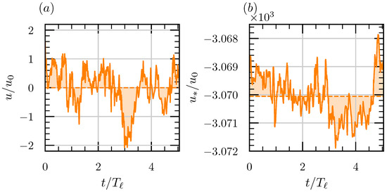
Figure 1. Temporal evolution of normalized velocity component in forced HIT at the domain center: (a) $u/u_o$ in the original frame and (b) $u_{*}/u_0$ in the rotating frame and at a phase $\varphi =\pi /4$. In (a), a dashed line style is used to represent the temporal average, which is null in HIT, whereas in (b), it is used for the phase average, which has a value of $-3.07\times {10}^3$.

With the purpose of corroborating the above, the probability distribution function, pdf, of each of the different velocity components in the original and in the rotating frame, is assessed. In HIT, these pdfs should be independent of time and space. Furthermore, they should agree for them to be invariant under proper rotations and reflections. Figure 2a compares the pdf of $u/u_o$ based on spatial information collected in two different instances and based on temporal information in two different positions. As seen from the figure, the agreement in the former and the latter implies, respectively, statistically stationarity and homogeneity. In addition, Figure 2a also displays the pdf of $v/u_o$ and of $w/u_0$ based on spatial information for one of the considered instances. As anticipated, these pdfs are also in agreement with the spatial-based pdf of $u/u_0$. Note that for a large enough number of events, complete overlapping between all curves is expected. In fact, the coincidence of the spatial- and temporal-based pdfs corroborates the ergodic hypothesis in turbulent flows that are both statistically stationary in time and homogeneous in space [19]. Note as well that the temporal-based information for estimating the pdfs appears to be particularly lacking. This is more easily discernible in the standard deviation, std, corresponding to the different pdfs; see Figure 2c.

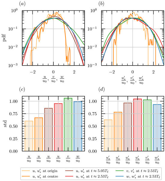
Figure 2. Probability distribution function, pdf, and standard deviation, std, in forced HIT: (a,c) $u/u_0$, $v/u_0$ and $w/u_0$, and (b,d) $u_{*}^{\prime }/u_0$, $v_{*}^{\prime }/u_0$ and $w_{*}^{\prime }/u_0$ at a phase $\varphi =\pi /4$. Yellow and orange colors are used to identify temporal-based information collected at the start and at the center of the spatial domain. Lines colored in red, green, and blue correspond to spatial-based information collected at $t/T_{\ell }\approx 2.53$, whereas brown corresponds to spatial-based information collected at $t/T_{\ell }\approx 5.05$.

Similar observations are made for the pdfs of the fluctuating velocity components at a phase after the time-periodic change of observer; see Figure 2b. In fact, there is even better agreement between the pdfs of $u_{*}^{\prime }/u_0$, $v_{*}^{\prime }/u_0$ and $w_{*}^{\prime }/u_0$ at $\varphi =\pi /4$. This improvement is attributed to the fact that there are more varied events in the sample space after the Euclidean transformation. This is also reflected in the stds shown in Figure 2d. In short, Figure 1 and Figure 2 exhibit HIT from the perspective of two different observers, highlighting that ${\left.{\mathit{u}}_{*}^{\prime }\right|}_{\varphi }$ is objective and that statistical symmetries such as stationarity and homogeneity are still preserved after a change of observer. Note that the last observation, although interesting, is not really surprising and can be seen as another indicator about the objectivity of the fluctuating field. For example, consider a homogeneous vector field which is frame-indifferent. Even after a change of observer, such a vector would retain this symmetry (homogeneity) since it is length-preserving.

3.2. Pressure-Driven TC Flow

The objectivity of the fluctuating velocity field and the Reynolds stress tensor is now investigated for plane TC flow. Compared to HIT, canonical wall-bounded turbulent flows are more accessible in the sense that there is a clear source of energy—the gradient of the mean velocity—entering the turbulent cascade [20]. A TC flow is also characterized by being inhomogeneous and having different Reynolds stress anisotropy states at different distances from the wall (see, e.g., [21,22]).

Figure 3 shows the temporal evolution of the velocity in the streamwise direction, u, and of the corresponding transformed velocity component, $u_{*}$, at $\varphi =\pi /4$ and after performing the 2D time-periodic change of observer. The signals are taken at the center of two wall-normal planes: one in the viscous wall region at $y{u}_{\tau }/\nu \approx 15$—where the streamwise variance is known to attain a maximum [23,24]—and another in the outer layer at $y/h\approx 0.8$. Figure 3a,b highlight some expected outcomes in TC flow. There are larger and more frequent velocity fluctuations in the near-wall region than in the channel core. Also, in the latter, the mean velocity is larger, as the total mean shear is noticeably less pronounced. Regarding the transformed velocity signals displayed in Figure 3c,d, it is interesting to note the difference in the phase average values and how this corresponds to the transformation rule (12). Despite both signals having the same deterministic component owing to the change of reference frame, they differ due to the modulation of the different mean components in the original inertial frame; see the first and second term in Equation (12), respectively.

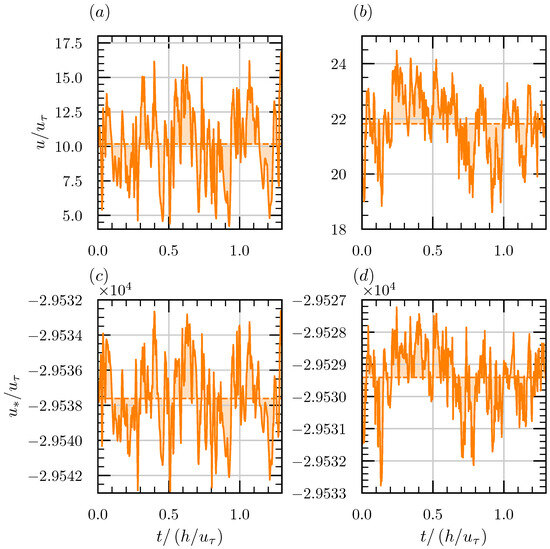
Figure 3. Temporal evolution of normalized velocity component in a pressure-driven TC flow: $u/u_{\tau }$ in the original frame and at the center of a wall-normal plane at (a) $y{u}_{\tau }/\nu \approx 15.36$ and (b) $y/h\approx 0.80$, and $u_{*}/u_{\tau }$ in the rotating frame, at a phase $\varphi =\pi /4$, and at the center of a wall-normal plane at (c) $y{u}_{\tau }/\nu \approx 15.36$ and (d) $y/h\approx 0.80$. In (a,b), a dashed line style is used to represent the temporal average, with respective values of $10.17$ and $21.82$, whereas in (c,d), it is used for the phase average, with approximate respective values of $-2.954\times {10}^4$ and $-2.953\times {10}^4$.

Now, let us consider the pdf of the different fluctuating velocity components for the same wall-normal positions, both in the original frame and in the rotating one. For the latter, once again the pdfs correspond to a phase $\varphi =\pi /4$. As in Section 3.1, some of the presented pdfs are solely based on temporal information, while others on spatial information. Figure 4a,c show the pdfs in the original frame. As can be seen, there is good agreement between the temporal- and spatial-based curves corresponding to $u^{\prime }$, showing that the flow is statistically homogeneous in the streamwise and spanwise directions and also statistically stationary. This also means that the ergodic hypothesis is fulfilled at both wall-normal positions. In addition, and as expected, there is a larger degree of anisotropy close to the wall than towards the channel center; see also the barycentric map [25] in Figure 5. A barycentric map is a linear map used to represent states of turbulence and is based on the analysis of the Reynolds stress anisotropy tensor [26]. As seen in Figure 5, close to the wall, the turbulence has just departed from the two-component limit (the variance in the wall-normal direction is starting to increase), whereas close to the channel center, the turbulence is approaching the axisymmetric expansion limit, with the variance in the streamwise direction still being larger than the others. See, e.g, Simonsen and Krogstad [27] for further details about the terminology used to characterize states of turbulence. With respect to the pdfs corresponding to the fluctuations in the transformed velocity components, see Figure 4b,d, it seems that the statistical symmetries (stationarity and homogeneity along $x_{*}$ and $z*$) are indeed carried over after the Euclidean transformation. Moreover, although at both wall-normal positions $v_{*}^{\prime }\equiv v^{\prime }$ has a shorter tail compared to the others, as shown in Figure 5, the turbulence anisotropy remains invariant after the change of observer. This is expected considering that the states of turbulence are defined in terms of the eigenvalues of the Reynolds stress anisotropy tensor [25], which is objective. This is the case precisely because it depends on the Reynolds stress tensor and its trace. In consequence, Figure 5 also reflects the material frame indifference of the Reynolds stress tensor.

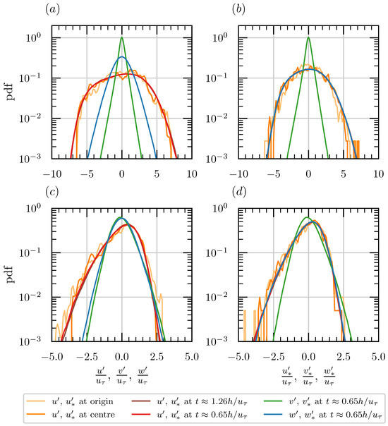
Figure 4. Probability distribution function, pdf, in a pressure-driven TC flow: $u^{\prime }/u_{\tau }$, $v^{\prime }/u_{\tau }$ and $w^{\prime }/u_{\tau }$ in the original frame and at (a) $y{u}_{\tau }/\nu \approx 15.36$ and at (c) $y/h\approx 0.80$; $u_{*}^{\prime }/u_{\tau }$, $v_{*}^{\prime }/u_{\tau }$ and $w_{*}^{\prime }/u_{\tau }$ in the rotating frame at a phase $\varphi =\pi /4$ and at (b) $y{u}_{\tau }/\nu \approx 15.36$ and at (d) $y/h\approx 0.80$. Yellow and orange colors are used to identify temporal-based information collected at the start and at the center of the respective wall-normal plane. Lines colored in red, green, and blue correspond to spatial-based information collected at $t{u}_{\tau }/h\approx 0.65$, whereas brown corresponds to spatial-based information collected at $t{u}_{\tau }/h\approx 1.26$.

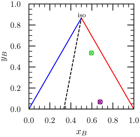
Figure 5. State of turbulence in a barycentric map [25]. Purple and green markers are used to denote the states of turbulence at $y{u}_{\tau }/\nu \approx 15.36$ and $y/h\approx 0.80$, whereas ‘∘’ and ‘×’ markers are used for states based on the Reynolds stress tensor in the original frame and in the rotating one, respectively. In the map, blue and red lines are used to identify the axisymmetric contraction and expansion limits, two-component states are found at the base, plane strain turbulence is represented by the dashed line, and isotropic turbulence is labeled as “iso”, with the barycentric coordinates $\left(x_B,y_B\right)=1/2,\sqrt{3}/2$.

Finally, let us discuss the only non-zero covariance, cov, in plane TC flow, i.e., the shear Reynolds stress. As shown in Figure 6, $u_{*}^{\prime }<0,v_{*}^{\prime }>0$ and $u_{*}^{\prime }>0,v_{*}^{\prime }<0$ events—analogous to the traditional sweeps and ejections [28,29] in the original frame—are predominant with a larger degree of correlation close to the wall than to the core. Nonetheless, the correlations at both wall-normal positions appear to have diminished compared to cov$(u^{\prime },v^{\prime })$. Compare Figure 6a,c with Figure 6b,d. This is because $u_{*}^{\prime }$ involves modulations of both $u^{\prime }$ and $w^{\prime }$, and cov$\left(w^{\prime }{v}^{\prime }\right)=0$. It is also remarked that, for the variances, the same statistical symmetries seen in cov$\left(u^{\prime }{v}^{\prime }\right)$ are carried over to cov$\left(u_{*}^{\prime }{v}_{*}^{\prime }\right)$ after the 2D time-periodic change of observer. In summary, Figure 3, Figure 4, Figure 5 and Figure 6 underline the objectivity of the fluctuating velocity and Reynolds stress tensor fields at a phase $\varphi$. Consistent with Section 3.1, the figures also show that the original statistical symmetries for the objective fields are preserved after the change of observer. From the figures, it is also clear that the well-known conclusions about TC flow in the inertial frame may not necessarily hold in a rotating one.

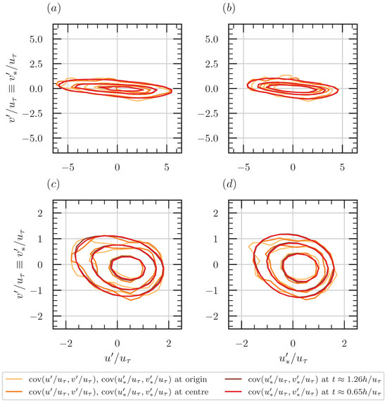
Figure 6. Joint pdf for finding the covariance, cov, in a pressure-driven TC flow of $u^{\prime }/u_{\tau }$ and $v^{\prime }/u_{\tau }$ in the original frame and at (a) $y{u}_{\tau }/\nu \approx 15.36$ and at (c) $y/h\approx 0.80$; $u_{*}^{\prime }/u_{\tau }$ and $v_{*}^{\prime }/u_{\tau }$ in the rotating frame, at a phase $\varphi =\pi /4$, and at (b) $y{u}_{\tau }/\nu \approx 15.36$ and at (d) $y/h\approx 0.80$. Yellow and orange colors are used to identify temporal-based information collected at the start and at the center of the respective wall-normal plane. Line colored in red corresponds to spatial-based information collected at $t{u}_{\tau }/h\approx 0.65$, whereas brown corresponds to spatial-based information collected at $t{u}_{\tau }/h\approx 1.26$. The approximate values of cov in (a), (b), (c), and (d) are −0.66, −0.47, −0.21, and −0.16, respectively.

4. Closing Remarks

In this paper, the frame indifference of typical turbulent fields is assessed after a time-periodic Euclidean transformation. Taking inspiration from Speziale [14], it is shown that the phase-averaged fluctuating velocity and Reynolds stress tensor fields are objective; see transformation rules (13) and (14). This is corroborated in a practical manner by examining one-point statistics of two canonical flow configurations: forced HIT and pressure-driven plane TC flow. The results also elucidate that, although different observers may not necessarily agree on their findings about the flows, statistical symmetries such as homogeneity, stationarity, and isotropy displayed by the objective fields are preserved after a change of observer. Altogether, this work draws attention to the validity of the objectivity axiom from the perspective of a statistical description of turbulent flows. It is also a first step toward the use of the principle of material frame indifference for the testing of hypotheses and models in turbulence. In particular, the fact that the Reynolds stress tensor is objective under a time-periodic change of observer has important implications for validating second-order closures in turbulence modeling.

Finally, with respect to the relevance of the objectivity axiom and the use of rotating frames in turbulence, it is worth emphasizing that beyond the important matter of generality—that is, insight about turbulence should not be restricted to inertial frames of reference—there are also practical reasons for considering rotating frames. Firstly, as in the case of a canonical channel flow, where it is convenient to consider an inertial frame aligned with the mean shear flow direction, for other flows, the use of a rotating frame may be more appropriate. For example, let us discuss the linear velocity field

$$\mathit{u}\left(\mathit{x},t\right)=\mathsf{A}\left(t\right)\mathit{x},\mathsf{A}=\left[\begin{array}{ccc}sin\left(4t\right)& -2-cos\left(4t\right)& 0\\ 2-cos\left(4t\right)& -sin\left(4t\right)& 0\\ 0& 0& 0\end{array}\right],$$

(16)

which is analogous to the one presented in Haller [30] for positive vorticity. In the inertial frame $\mathit{x}$, the velocity field (16) is unsteady. In addition, it has a fixed elliptical stagnation point at the origin and closed streamlines [2], typically associated with vortical motion. Conversely, when passing to the rotating frame

$${\mathit{x}}_{*}=\mathsf{Q}\left(t\right)\mathit{x},\mathsf{Q}=\left[\begin{array}{ccc}cos\left(2t\right)& sin\left(2t\right)& 0\\ -sin\left(2t\right)& cos\left(2t\right)& 0\\ 0& 0& 1\end{array}\right],$$

(17)

according to the transformation rules (1) and (3), the velocity field in ${\mathit{x}}_{*}$ is given by

$${\mathit{u}}_{*}\left({\mathit{x}}_{*},t\right)=\left(\dot{\mathsf{Q}}+\mathsf{Q}\mathsf{A}\right){\mathsf{Q}}^{\mathrm{T}}{\mathit{x}}_{*}\equiv \mathsf{B}{\mathit{x}}_{*},\mathsf{B}=\left[\begin{array}{ccc}0& -1& 0\\ -1& 0& 0\\ 0& 0& 0\end{array}\right],$$

(18)

which represents a steady flow with a saddle point at its center. Thus, the frame change (17) not only eliminates the temporal dependency but also allows us to realize the correct material behavior, that is, a rotating saddle point [31]. The convenience of using a rotating frame for flows within rotating devices is evident (e.g., stirred tanks and centrifugal pumps); however, this may also be the case for more traditional and well-studied flows such as pipes and channels if rotating [32,33] and strong curvature effects [34,35] are considered. Lastly, note that examples (16)–(18) also highlight another practical reason for considering changes to non-inertial frames and for having awareness about objectivity in general: typical tools for flow visualization such as streamlines may misdiagnose material behavior, e.g., in this case, the identification of a vortex instead of a hyperbolic structure. The study of coherent structures in turbulence from the perspective of material barriers has gained renewed interest in recent years (see, e.g., [36,37]), underlying the importance of the principle of material frame indifference for the community. In a similar manner, knowledge about the (non-)objectivity of turbulent fields can be used for testing hypotheses and models in turbulence. For instance, think about the different scaling laws proposed for the inner peak of the streamwise velocity variance in wall-bounded turbulent flows; see, e.g., discussion in Hwang [38]. The use of objectivity for the testing of hypotheses and models in wall-bounded turbulence is seen as a promising research direction and warrants future studies.

References

- Monin, A.S.; Yaglom, A.M. Statistical Fluid Mechanics, Vol. I: Mechanics of Turbulence; MIT Press: Cambridge, MA, USA, 1971. [Google Scholar]
- Haller, G. Transport Barriers and Coherent Structures in Flow Data; Cambridge University Press: Cambridge, UK, 2023. [Google Scholar] [CrossRef]
- Murdoch, A.I. Objectivity in classical continuum physics: A rationale for discarding the ‘principle of invariance under superposed rigid body motions’ in favour of purely objective considerations. Contin. Mech. Thermodyn. 2003, 15, 309–320. [Google Scholar] [CrossRef]
- Murdoch, A.I. On criticism of the nature of objectivity in classical continuum physics. Contin. Mech. Thermodyn. 2005, 17, 135–148. [Google Scholar] [CrossRef]
- Liu, I.S. On Euclidean objectivity and the principle of material frame-indifference. Contin. Mech. Thermodyn. 2004, 16, 177–183. [Google Scholar] [CrossRef]
- Liu, I.S. Further remarks on Euclidean objectivity and the principle of material frame-indifference. Contin. Mech. Thermodyn. 2005, 17, 125–133. [Google Scholar] [CrossRef]
- Oldroyd, J.G. On the formulation of rheological equations of state. Proc. R. Soc. Lond. A 1950, 200, 523–541. [Google Scholar] [CrossRef]
- Speziale, C.G. A Review of Material Frame-Indifference in Mechanics. Appl. Mech. Rev. 1998, 51, 489–504. [Google Scholar] [CrossRef]
- Lumley, J.L. Toward a turbulent constitutive relation. J. Fluid. Mech. 1970, 41, 413–434. [Google Scholar] [CrossRef]
- Lumley, J.L. Turbulence Modeling. J. Appl. Mech. 1983, 50, 1097–1103. [Google Scholar] [CrossRef]
- Marusic, I.; Monty, J.P. Attached Eddy Model of Wall Turbulence. Annu. Rev. Fluid Mech. 2019, 51, 49–74. [Google Scholar] [CrossRef]
- Gurtin, M.E.; Fried, E.; Anand, L. The Mechanics and Thermodynamics of Continua; Cambridge University Press: Cambridge, UK, 2010. [Google Scholar] [CrossRef]
- Pope, S.B. Turbulent Flows; Cambridge University Press: Cambridge, UK, 2000. [Google Scholar] [CrossRef]
- Speziale, C.G. Invariance of turbulent closure models. Phys. Fluids 1979, 22, 1033–1037. [Google Scholar] [CrossRef]
- Goldstein, H.; Poole, C.P.; Safko, J.L. Classical Mechanics; Pearson: London, UK, 2002. [Google Scholar]
- Li, Y.; Perlman, E.; Wan, M.; Yang, Y.; Meneveau, C.; Burns, R.; Chen, S.; Szalay, A.; Eyink, G. A public turbulence database cluster and applications to study Lagrangian evolution of velocity increments in turbulence. J. Turbul. 2008, 9, 1–29. [Google Scholar] [CrossRef]
- Graham, J.; Kanov, K.; Yang, X.I.A.; Lee, M.K.; Malaya, N.; Lalescu, C.C.; Burns, R.; Eyink, G.; Szalay, A.; Moser, R.D.; et al. A Web services accessible database of turbulent channel flow and its use for testing a new integral wall model for LES. J. Turbul. 2016, 17, 181–215. [Google Scholar] [CrossRef]
- Jiménez, J. Cascades in Wall-Bounded Turbulence. Annu. Rev. Fluid Mech. 2012, 44, 27–45. [Google Scholar] [CrossRef]
- Galanti, B.; Tsinober, A. Is turbulence ergodic? Phys. Lett. A 2004, 330, 173–180. [Google Scholar] [CrossRef]
- Jiménez, J. Near-wall turbulence. Phys. Fluids 2013, 25, 101302. [Google Scholar] [CrossRef]
- Lee, M.; Moser, R.D. Direct numerical simulation of turbulent channel flow up to Reτ ≈ 5200. J. Fluid. Mech. 2015, 774, 395–415. [Google Scholar] [CrossRef]
- Hoyas, S.; Oberlack, M.; Alcántara-Ávila, F.; Kraheberger, S.V.; Laux, J. Wall turbulence at high friction Reynolds numbers. Phys. Rev. Fluids 2022, 7, 014602. [Google Scholar] [CrossRef]
- Sreenivasan, K.R. The turbulent boundary layer. In Frontiers in Experimental Fluid Mechanics; el Hak, M.G., Ed.; Springer: Berlin/Heidelberg, Germany, 1989; pp. 159–209. [Google Scholar] [CrossRef]
- Smits, A.J.; Hultmark, M.; Lee, M.; Pirozzoli, S.; Wu, X. Reynolds stress scaling in the near-wall region of wall-bounded flows. J. Fluid. Mech. 2021, 926, A31. [Google Scholar] [CrossRef]
- Banerjee, S.; Krahl, R.; Durst, F.; Zenger, C. Presentation of anisotropy properties of turbulence, invariants versus eigenvalue approaches. J. Turbul. 2007, 8, 1–27. [Google Scholar] [CrossRef]
- Lumley, J.L.; Newman, G.R. The return to isotropy of homogeneous turbulence. J. Fluid. Mech. 1977, 82, 161–178. [Google Scholar] [CrossRef]
- Simonsen, A.J.; Krogstad, P.A. Turbulent stress invariant analysis: Clarification of existing terminology. Phys. Fluids 2005, 17, 088103. [Google Scholar] [CrossRef]
- Wallace, J.M.; Eckelmann, H.; Brodkey, R.S. The wall region in turbulent shear flow. J. Fluid. Mech. 1972, 54, 39–48. [Google Scholar] [CrossRef]
- Willmarth, W.W.; Lu, S.S. Structure of the Reynolds stress near the wall. J. Fluid. Mech. 1972, 55, 65–92. [Google Scholar] [CrossRef]
- Haller, G. An objective definition of a vortex. J. Fluid. Mech. 2005, 525, 1–26. [Google Scholar] [CrossRef]
- Haller, G. Lagrangian coherent structures. Annu. Rev. Fluid Mech. 2015, 47, 137–162. [Google Scholar] [CrossRef]
- Xiao, M.; Ceci, A.; Orlandi, P.; Pirozzoli, S. Direct numerical simulation of drag reduction in rotating pipe flow up to Reτ ≈ 3000. J. Fluid. Mech. 2024, 996, A24. [Google Scholar] [CrossRef]
- Ceci, A.; Pirozzoli, S. Direct numerical simulation study of turbulent pipe flow with imposed radial rotation. J. Fluid. Mech. 2025, 1004, A15. [Google Scholar] [CrossRef]
- Soldati, G.; Orlandi, P.; Pirozzoli, S. Reynolds number effects on turbulent flow in curved channels. J. Fluid. Mech. 2025, 1007, A15. [Google Scholar] [CrossRef]
- Orlandi, P.; Soldati, G.; Pirozzoli, S. Effects of curvature on turbulent flow in concentric annuli and curved channels. J. Fluid. Mech. 2025, 1009, A29. [Google Scholar] [CrossRef]
- Haller, G.; Katsanoulis, S.; Holzner, M.; Frohnapfel, B.; Gatti, D. Objective barriers to the transport of dynamically active vector fields. J. Fluid. Mech. 2020, 905, A17. [Google Scholar] [CrossRef]
- Aksamit, N.O.; Haller, G. Objective momentum barriers in wall turbulence. J. Fluid. Mech. 2022, 941, A3. [Google Scholar] [CrossRef]
- Hwang, Y. Near-wall streamwise turbulence intensity as Reτ → ∞. Phys. Rev. Fluids 2024, 9, 044601. [Google Scholar] [CrossRef]
Disclaimer/Publisher’s Note: The statements, opinions and data contained in all publications are solely those of the individual author(s) and contributor(s) and not of MDPI and/or the editor(s). MDPI and/or the editor(s) disclaim responsibility for any injury to people or property resulting from any ideas, methods, instructions or products referred to in the content. |
© 2026 by the authors. Licensee MDPI, Basel, Switzerland. This article is an open access article distributed under the terms and conditions of the Creative Commons Attribution (CC BY) license.