Data Descriptor

Climate Data to Support the Adaptation of Buildings to Climate Change in Canada

Construction Research Center, National Research Council Canada, 1200 Montreal Road, Ottawa, ON K1A 0R6, Canada
*
Author to whom correspondence should be addressed.
Submission received: 16 February 2022 / Revised: 26 March 2022 / Accepted: 29 March 2022 / Published: 6 April 2022

Abstract

:
Climate change will continue to bring about unprecedented climate extremes in the future, and buildings and infrastructure will be exposed to such conditions. To ensure that new and existing buildings deliver satisfactory performance over their design lives, their performance under current and future projected climates needs to be assessed by undertaking building simulations. This study prepares climate data needed for building simulations for 564 locations by bias-correcting the Canadian Regional Climate Model version 4 (CanRCM4) large ensemble (LE) simulations with reference to observations. Technical validation results show that bias-correction effectively reduces the bias associated with CanRCM4-LE simulations in terms of their marginal distributions and the inter-relationship between climate variables. To ensure that the range of projected climate change impacts are encompassed within these data sets, and to furthermore provide building moisture and energy reference years, the reference year files were prepared from bias-corrected CanRCM4-LE simulations and are comprised of a typical meteorological year for building energy applications, a typical and extreme moisture reference year, a typical downscaled year, an extreme warm year, and an extreme cold year.
Dataset:https://osf.io/guwqc/ (accessed on 30 January 2022).
Dataset License: CC0.

1. Introduction

Climate change is one of the most significant challenges Canada and countries around the globe have faced and are facing. Since 1948, average temperatures in Canada have increased by 1.7 °C, at a rate about twice the global average. The total precipitation has also increased in most parts of Canada. In addition to the changes in average climate, extreme events such as heat spells, thunderstorms, flooding, and wildfires have increasingly become more frequent and intense [1,2]. It is projected that climate change will continue to affect Canada’s climate regardless of the amount of greenhouse gas emissions made by the global community in the future. By the end of the 21st century, the average temperatures across Canada will increase by 1.8 °C even under the most conservative projections of future greenhouse gas emissions, and can increase by up to 6.3 °C under the least conservative greenhouse gas emissions projections [3]. Similarly, the current 20-year return period highest daily annual temperatures are projected to become 5-year return period events by the mid-21st century even under the most conservative projections of future greenhouse gas emissions, while they can become a 2-year return period event under the least conservative projections of greenhouse gas emissions [3]. As a result, buildings and infrastructure across Canada will be exposed to drastically different climatic conditions and extreme events than experienced historically, and need to be designed taking into account the long-term non-stationarity in climate [4].
Building simulations are important tools for assessing the performance of buildings under current and future projected climates. By undertaking hygrothermal simulations, Ref. [5] from Sweden estimated potential moisture accumulation in the outermost layer of the façade for a typical wood frame wall construction under historical and future, projected wind-driven rain loads. In [6] the potential future impacts of climate change on antiquities stored in two historic buildings, one located in the Netherlands and the other located in Belgium, are assessed by undertaking building simulations. Increases in indoor temperatures by up to 2 °C and indoor relative humidity by up to 2.6% are projected by the end of the 21st century, highlighting the danger of moisture damage to artifacts stored in the buildings. In [7] thermal performance of the Roland Levinsky Building in the UK is analyzed under projected climate change influences by undertaking whole building simulations. The results indicate that without additional cooling, indoor temperatures are expected to rise in the building in the future, affecting the thermal comfort of the occupants. Several other studies incorporating building simulations have been performed to assess the performance of building envelopes [8,9,10,11,12,13,14,15].
Climate data incorporating the future effects of climate change are an essential component when conducting building simulations that permit the assessment of the long-term future performance of buildings [16,17]. Typically, hourly or more frequent time-series of multiple climate variables are needed. Whilst building energy simulations can be conducted with information on temperature, dew point, pressure, wind speed and direction, and solar radiation, hygrothermal simulations additionally require rainfall to accurately model the transport of moisture within the wall assemblies [18]. In an effort to reduce the computational costs associated with running building models over long periods of time, simulations are performed over subsets of long-term climate data, typically over one year, referred to as reference weather years (RWYs) [13]. Depending on the application, either typical or extreme years are chosen as RWYs. The Canadian Weather Year for Energy Calculation (CWEC) database from Environment and Climate Change Canada [19], for example, used extensively by building practitioners in Canada for building energy applications, contains typical RWYs prepared following the methodology outlined in [20]. Several other RWYs such as Weather Year for Energy Calculations (WYEC) [21], International Weather Year for Energy Calculation (IWEC) [22], Typical Meteorological Year 2 [23], and others reviewed in [16] have been used for building energy applications.
Extreme RWYs have been used for assessing peak energy loads in buildings [24]. For building overheating assessments, extreme RWYs are of interest and, again, a range of them have been used, such as Design Summer Year [23], Design Reference Year [24], Summer Reference Years [25], Extreme Meteorological Year [26], Summer Weather Years [14], and others reviewed in [16]. For assessing hygrothermal performance of wall assemblies, an extreme RWY with the greatest potential for moisture damage in buildings is chosen. In [18] the year with the highest Moisture Index [27] is used as the RWY for evaluating the performance of four hygrothermal simulation tools in simulating moisture-related damage in four different wall assemblies for three (3) Canadian city locations: Ottawa, Vancouver, and Calgary. In [28] the year with a 10% failure level in terms of Climatic index and RHT index is selected as the RWY for assessing the hygrothermal performance of three different wall assemblies in four cities located in Switzerland.
As opposed to considering either a typical or an extreme year, Ref. [29] demonstrated the need to select both typical and extreme years for building simulations, by selecting three RWYs: typical, extreme cold, and extreme warm years based on dry bulb temperatures. Such an approach effectively captures the range of climatic conditions and building energy responses demonstrated by an ensemble of long-term climate projections from multiple regional climate models. In [13] the selection of the three RWYs is made based on dry bulb temperature, equivalent temperature, and precipitation, and it was found that in the case of a pre-fabricated wooden frame wall, the RWYs selected based on dry bulb temperature were able to closely replicate the moisture content, relative humidity, temperature and mould growth rate in the façade and insulation layers of the wall assembly obtained from the long-term climate datasets. Since then, a number of studies have used this method to identify typical and extreme RWYs, enabling users to effectively capture the uncertainty from climate projections with substantially reduced computational costs [24,30,31].
Building simulation data have been prepared for locations around the globe. For example, the American Society of Heating, Refrigerating and Air-Conditioning Engineers (ASHRAE) weather data center (https://www.ashrae.org/technical-resources/bookstore/weather-data-center (accessed on 30 January 2022)) provides, for a fee, typical-year building simulation files for 3012 worldwide locations outside the United States and Canada. The Pacific Climate Impacts Consortium (PCIC) provides “future shifted weather files” for 466 locations in Canada by means of a Wx file tool (https://services.pacificclimate.org/demo/wx-files/app/ (accessed on 30 January 2022)). The Climate Change World Weather File Generator for World-Wide Weather Data—CCWorldWeatherGen (https://energy.soton.ac.uk/ccworldweathergen/ (accessed on 30 January 2022)) provides users with future projected climate files and typical RWY files for locations across the globe. Several other studies [32,33,34,35,36] have prepared building simulation files incorporating the future projected effects of climate change.
The morphing method has been most often used to prepare future projected building simulations files. In this method, “morphed” future projections are prepared by adjusting observations based on future projected changes from a global or regional climate model. In the present work, current and future projected building simulation datasets were prepared for 564 locations widely distributed across Canada by using bias-corrected and dynamically downscaled regional climate model projections. The unique aspects of this database over similar existing databases are: (i) Each climate file includes variables sufficient for undertaking both hygrothermal and whole building simulations—most existing databases only include variables needed for whole building simulations; (ii) both typical and extreme RWYs are prepared with indices relevant for different building applications, which will allow the use of data for several applications such as overheating, hygrothermal performance, energy use, peak energy demand, and encompassing variability in projected climate change impacts etc.—existing databases mostly provide typical or extreme RWYs; (iii) climate files are prepared directly from regional climate model projections, which makes it possible to account for complex distributional changes in future climate.
The layout of this paper is as follows: the locations considered for data generation are described in Section 2, followed by the data and methods used in Section 3, a discussion on the accuracy of key steps of the methodology in Section 4, and conclusions in Section 5.

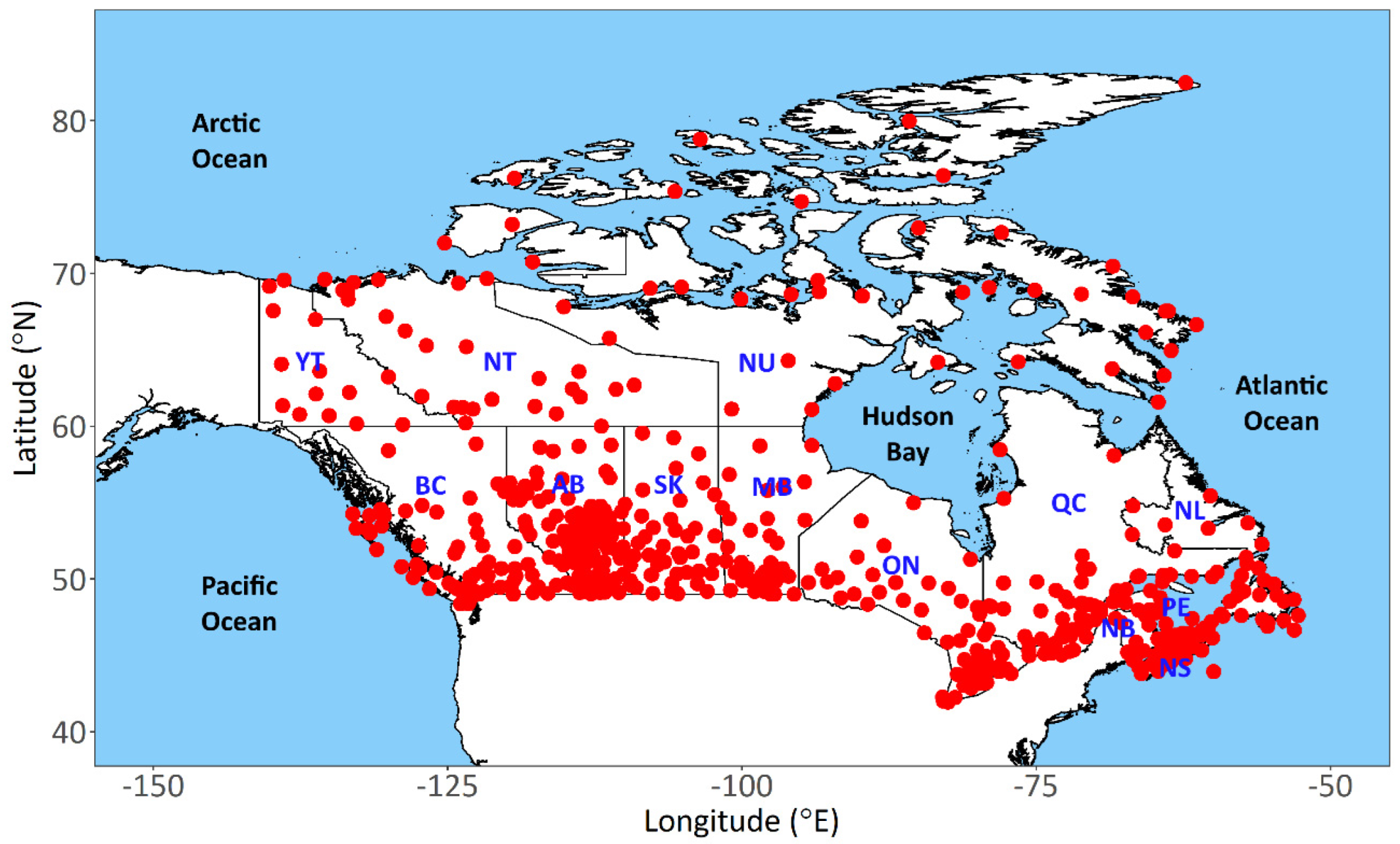
2. Locations Considered for Data Generation

The building simulation files were generated for 564 locations, shown in Figure 1, which were considered in the most recent 2020 version of the Canadian Weather Energy and Engineering Datasets (CWEEDS)/Canadian Weather Year for Energy Calculation (CWEC) datasets from Environment and Climate Change Canada (ECCC) (https://climate.weather.gc.ca/prods_servs/engineering_e.html (accessed on 30 January 2022)). The locations were carefully chosen in the CWEEDS/CWEC database to represent different climate types over the Canadian landmass whilst making the best possible use of available observational records from ECCC’s climate databases [19]. There is a higher number of locations in the southern parts of Canada than in the northern parts, given the greater availability of observational records for southern Canada. Of the 564 locations, 13 are located in the Yukon Territory (YT), 32 in the Northwest Territories (NT), 37 in Nunavut (NU), 78 in British Columbia (BC), 102 in Alberta (AB), 44 in Saskatchewan (SK), 39 in Manitoba (MB), 61 in Ontario (ON), 81 in Quebec (QC), 13 in New Brunswick (NB), 29 in Nova Scotia (NS), 7 in Prince Edwards Island (PE), and 28 in the Newfoundland and Labrador (NL) provinces of Canada.
The elevation, historical wind speed, relative humidity, temperature, and global horizontal irradiance amongst these locations vary from 1 to 2543 m, 1 to 10 m/s, 60 to 90%, −17 to 12 °C, and 302 to 586 kJ·h/m2, respectively, between 1998 and 2017 as per the 2020 CWEEDS database.

3. Methodology

The generated building simulation data consist of typical and extreme RWY files for 564 locations forming part of ECCC’s CWEEDS/CWEC database. The climate variables in the RWY files are sufficient for undertaking both hygrothermal and whole building simulations, and include hourly values of air temperature (TEMP), relative humidity (RHUM), atmospheric pressure (PRES), snow-cover flag (SNOWC), wind speed (WSP), wind direction (WDIR), total rainfall (RAIN), total cloud-cover (TCC), and global (GHI) as well as direct normal (DNI) and diffused horizontal (DHI) solar radiation, as listed in Table 1. The data are generated for a historical time-period of: 1991–2021; future time-periods are coincident with increases in global temperatures of: 0.5, 1.0, 1.5, 2.0, 2.5, 3.0 and 3.5 °C. The future time-periods with the aforementioned levels of global warming are calculated after an analysis of global averaged temperatures modelled by the Canadian Earth System Model, CanESM2, and are found to be: 2003–2033, 2014–2044, 2024–2054, 2034–2064, 2042–2072, 2051–2081, and 2064–2094, respectively.
The methodology followed consists of four steps, outlined in Figure 2 and explained hereafter.

3.1. Preparation of Database of Observations and Climate Model Simulations

A database of hourly observations and climate model simulations for the selected locations was prepared. Observations of hourly global horizontal irradiance, station pressure, dry bulb temperature, dew point temperature, and wind speed and direction were taken from ECCC’s 2020 CWEEDS database (https://climate.weather.gc.ca/prods_servs/engineering_e.html (accessed on 30 January 2022)). Observations of rainfall, total cloud-cover, and snow depth were not part of 2020 CWEEDS datasets, and as a consequence, they were collected from Environment Canada’s historical climate datasets, respectively: HLY03-123, HLY01-082, and DLY04-013 (https://climate.weather.gc.ca/historical_data/search_historic_data_e.html (accessed on 30 January 2022)). For the aforementioned variables, the historical observational records collected at climate gauging stations, and within 5 km of the CWEEDS stations, were merged by giving the greatest preference to those observations recorded closest to CWEEDS stations and subsequently, a lower preference to observations recorded farther away from the stations. If missing values were present in the merged observational time-series, they were supplied through quantile mapping of climate estimates from the Climate Forecast System Reanalysis (CFSR) [37] on the observations.
For preparing the database of current and future projected climates for the selected locations, a large ensemble of Canadian Regional Climate Model version 4 (CanRCM4-LE) simulations was used. The CanRCM4-LE was prepared by the dynamic downscaling of Canadian Earth System model large ensemble simulations (CanESM2-LE). CanESM2 is a global climate model with interactive atmosphere, ocean, sea ice, land, and carbon cycle components [38]. To prepare the CanESM2 large ensemble, a large initial condition ensemble consisting of 50 simulations was randomly initialized starting on 1 January 1950 from the 5 historical ensemble members, by selecting 10 random sets of cloud physics parameterizations in the model [39]. The historical simulations covered the time-period 1950–2004, and future projections over 2005–2100 were made using the Representative Concentration Pathway (RCP) 8.5 [40]. The CanESM2-LE simulations were dynamically downscaled from a geographical horizontal spacing of ~2.8° to ~0.44° using the CanRCM4 model to prepare the CanRCM4-LE. A subset of the CanRCM4-LE simulations comprising 15 realizations were archived in hourly time-steps by ECCC and were acquired for the purposes of this study. The CanRCM4-LE simulations have been used extensively to integrate climate resiliency in the design of buildings and core public infrastructure in Canada [41].
The CaRCM4-LE simulations for the 1991–2100 time-period, and comprising hourly global horizontal irradiance, total cloud cover, precipitation, u and v components of 10 m wind, relative humidity, temperature, atmospheric pressure, and daily solid precipitation and snow depth, were collected for the grid closest to the 564 locations for the purposes of this study [42].

3.2. Bias Correction of Climate Model Simulations

Bias-correction of climate variables was performed using trend preserving univariate (QDM) [43] and Multivariate Bias Correction with N-dimensional probability density function transform (MBCn) [44] methods. The QDM is a univariate bias-correction method that preserves climate-model-projected relative changes in the quantiles while at the same time correcting systematic biases in quantiles with respect to the observations. First, climate model projections, de-trended by quantile, are mapped on observations following equation 1 by quantile mapping and x m , p , d t b c ( t ) is calculated. Thereafter, climate-model-projected relative Equation (2) or additive changes in quantiles Δ m ( t ) are obtained, and combined with x m , p , d t b c ( t ) using multiplicative Equation (3) or additive operations to obtain the final bias-corrected future projections x m , p , b c ( t ) .
x m , p , d t b c = F o , h 1 [ F m , p ( t ) [ x m , p ( t ) ] ]
Δ m ( t ) = x m , p ( t ) F m , h 1 [ F m , p ( t ) [ x m , p ( t ) ] ]
x m , p , b c ( t ) = x m , p , d t b c ( t ) × Δ m ( t )
where, x m , p ( t ) ,   x m , p , d t b c ( t ) ,   x m , p , b c ( t ) are the raw, de-trended and bias-corrected, and final bias-corrected climate projections at time t, respectively; F m , p ( t ) ,   F m , h ( t ) ,   F o , h ( t ) are the cumulative distribution functions (CDFs) of the climate model future projections, historical simulations, and observations, respectively. Their respective inverse functions ( F 1 ) follow similar nomenclature.
The MBCn method extends the application of the QDM method in a multivariate context. First, the univariate distributions of climate projections were bias-corrected using the QDM method. Thereafter, the dependence structure of climate variables was corrected using an iterative process. At each iteration, the data were multiplied by random orthogonal rotation matrices to partially de-correlate the climate variables requiring correction. The QDM corrections were applied to the partially de-correlated data before they were re-correlated using the inverse random matrices. This process of rotation, QDM correction, and back-rotation was repeated until convergence was reached between the multivariate distributions of climate simulations and the reference dataset [45].
The climate variables from CanRCM4-LE simulations were bias-corrected with reference to observations. In this study, MBCn was chosen as the preferred method for bias-correction over QDM as it is able to correct the marginal distribution of variables as well as the dependence structure between them. All climate variables except GHI were bias-corrected using MBCn, as shown in Table 1. The QDM is preferred over MBCn to bias-correct GHI because the reshuffling of values in MBCn is found to modify the diurnal characteristics of GHI, resulting in unrealistic values for global, diffuse, and direct solar radiation. The QDM and MBCn methods were implemented using the MBC package [41] in the R programming language [44]. The bias-correction methods were calibrated individually for each month using data from the three months surrounding it. This implies that to calibrate the MBCn/QDM method for the month of January, data for the months of December, January and February were used and so on.
Finally, previous studies have shown that it is important to account for the internal variability of climate when applying bias-correction algorithms to an ensemble of climate model projections [45,46,47], otherwise, bias-correction can lead to an artificially reduced ensemble spread. In an effort to account for this, bias-correction methods were calibrated and predicted over different realizations of CanRCM4-LE to preserve the internal variability of climate simulations in the bias-corrected data.

3.3. Estimation of Direct and Diffused Components of Global Solar Radiation

As shown in Table 1, the direct (DNI) and diffuse (DHI) components of solar radiation are estimated from the bias-corrected GHI. The following steps were performed to achieve these values:
  • Hourly clearness index ( k T ) was calculated as the ratio of hourly GHI and extra-terrestrial solar radiation, which was calculated using equations provided in [48].
  • The values of k T were used to calculate the diffused fraction k d using Equation (4) [49].
    k d = { 1 0.249 k t f o r   k T < 0.35 1.557 1.84 k T f o r   0.35 k T < 0.75 0.177 f o r   k T 0.75 }
  • The DHI was calculated using Equation (5).
    D H I = G H I × k d
  • The values of DNI were calculated using Equation (6).
D N I = G H I D H I sin θ
where, θ is the hourly solar elevation angle.
It is known that in the early mornings and late evenings, when the solar elevation angle is low, global radiation is primarily comprised of diffuse radiation. To limit the amount of direct radiation as may be estimated at low solar elevation angles, previous studies, such as those by [15,19], have considered solar angle thresholds (such as 5°) below which the global solar radiation is considered to be fully comprised of diffuse radiation. If a limiting threshold value is not used, it can result in unrealistic DNI values in the early-morning and late-evening hours.
In this study, instead of using a user-defined threshold for solar angle, the approach adopted by International Energy Agency Annex 80 [50] was used to calculate the limiting (maximum) value of DNI for each hour of the day, as it allows for a physically based (dependent on local turbidity and elevation) estimation of direct and diffused components of solar radiation which can be uniformly applied at locations around the globe. The approach uses the Linke turbidity factor and elevation of a location to calculate the limiting value of DNI [51]. The Linke turbidity factor is an approximation to modelling the atmospheric absorption and scattering of solar radiation under clear skies. It describes the optical thickness of the atmosphere due to absorption by water vapor, and the absorption and scattering by aerosol particles relative to a dry and clean atmosphere, and thus permits summarizing the turbidity of the atmosphere and hence the attenuation of direct beam solar radiation [52,53]. The larger the value of the Linke turbidity factor, the larger the attenuation of radiation by a clear-sky atmosphere.
The estimates of Linke turbidity values for the 564 CWEEDS locations were taken from the 2010 gridded estimates provided in Solar Radiation Data (SoDa; http://www.soda-pro.com/help/general-knowledge/linke-turbidity-factor (accessed on 30 January 2022) [51]. The limiting value of direct irradiance on a horizontal surface (or limiting direct irradiance) for clear sky,   D N I l i m , is calculated as:
D N I l i m = I 0 × ε × sin γ s × e 0.8662 × T L × m × δ R a y l e i g h ( m )
where I 0 is the solar constant, ε is the correction used to allow the variation in sun−earth distance from its mean value, γ s is the solar elevation angle, T L is the Linke turbidity factor for an air mass equal to 2, m is the optical air mass at sea level, and δ R a y l e i g h ( m ) is the integrated Rayleigh optical thickness due to pure molecular scattering.
If the value of DNI calculated from equations 4–6 is above the hourly D N I l i m value, the DNI value is replaced by D N I l i m and DHI values are recalculated to ensure diffuse and direct components add up to the value of GHI.

3.4. Extraction of Reference Years from Long-Term Time-Series Data

3.4.1. Moisture Reference Year (MRY) for Hygrothermal Applications

When performing hygrothermal simulations, the wall assemblies are typically conditioned over a typical climate year before they are tested against an extreme climate year. A number of studies performed on Canadian cities have used this approach, and the conditioning and extreme years were selected based on the value of the Moisture Index (MI) [17,18,54,55,56,57]. The MI is referenced in the National Building Code of Canada [58] and the Guideline on design for durability of building envelopes in Canada [59] as a climate-based metric that permits conveying, for example, to building practitioners, the potential for moisture damage in wall assemblies.
The MI is an indicator of the potential for moisture damage in wall assemblies when exposed to an exterior climate [27]. The wetting and drying processes in a wall assembly, as indicated through the MI, are accounted for by means of the Wetting Index (WI) and the Drying Index (DI), respectively. The WI is defined as the average annual free wind-driven rain calculated using Equation (8), normalized across all years.
f w d r ( h ) = w s p ( h ) × r a i n ( h )
The DI, representing the drying processes, is defined as a function of the difference in the humidity levels between the saturation ( w s a t ) and ambient air conditions ( w a m b ) in the outdoors. The drying capacity at each hour is calculated following equation 9 before averaging to the annual time-scale, and normalizing across all years.
Δ w ( h ) = w s a t ( h ) w a m b ( h )
Finally, the MI is expressed as a combination of WI and DI as:
M I = W I 2 + ( 1 D I ) 2
Following the previously mentioned work and recommendations, for the present study, the median ranked year was selected in terms of MI as the conditioning year and the 10%-year (3rd year out of 31 years) as the extreme year for hygrothermal applications.

3.4.2. Typical Meteorological Year (TMY) for Building Energy Applications

For building energy applications, TMYs are prepared using the Sandia method [20] by concatenating twelve typical meteorological months selected based on Finkelstein−Schafer (FS) statistics. To calculate the FS statistic, daily values of climate parameters listed in Table 2 were compiled from the hourly time-series of global horizontal irradiance, temperature, dew point temperature (estimated from relative humidity and temperature), and wind speed. The climate parameters were attached with the relative weights provided in Table 2 following [20] to reflect the relative contribution of different climate variables in affecting the energy performance of buildings, and combined to calculate the daily FS statistic.
To prepare the TMY from daily FS statistic values, the cumulative distribution function (CDF) of daily FS statistic values from all long-term data was compared with the FS statistic CDF of each year and CanRCM4-LE run. The month with a CDF most closely matching the CDF of all long-term data is selected as the typical meteorological month. The CDFs are compared in terms of absolute mean difference in quantiles with 100 evenly spaced probabilities between 0 and 1, similar to what is reported in [29]. This process is repeated for all months from January to December to obtain the typical meteorological month for each calendar month. Finally, all typical meteorological months are combined to obtain the TMY.

3.4.3. Temperature Reference Years (TRYs) to Capture Climate Uncertainty

The TRYs were selected following the method demonstrated in [13,29], where a “typical downscaled year (TDY)”, “extreme cold year (ECY)”, and “extreme warm year (EWY)” were prepared by concatenating twelve typical, extreme cold, and extreme warm months, respectively. The typical, extreme cold, and extreme warm months were identified by following a procedure similar to that used in the preparation of TMY. For each month, the CDF of air temperature was compared with the CDF from all long-term data. Again, the difference in CDFs was calculated with the help of quantiles corresponding to 100 evenly spaced probabilities between 0 and 1. The year and CanRCM4-LE run with the least absolute difference from the CDF of data from all years was considered as the TDY. The ECY was chosen as the year having the minimum real (not absolute) difference from the CDF of data from all years, and the EWY is the year with the maximum real difference.

4. Results and Discussion

4.1. Efficiency of Bias-Correction

Use of the MBCn and QDM methods effectively reduces the bias associated with CanRCM4-LE-simulated climate variables. This is shown by means of Figure 3 and Figure 4, in which the Probability Density Functions (PDFs) of observations (black), raw CanRCM4-LE (blue), and bias-corrected CanRCM4-LE values (red) are shown, respectively, for the Toronto International Airport and Whitehorse International Airport locations. The PDFs presented are for air temperature, wind speed, relative humidity, and total cloud-cover, and were prepared for the time-period 1998–2017, over which observations as well as CanRCM-LE projections were available. It can be seen that the distribution of climate variables in bias-corrected CanRCM4-LE data is closer to the observations than the raw CanRCM4-LE data.
The performance of bias-correction over all 564 locations is summarized in Figure 5, where scatterplots of observations vs. raw (blue) and bias-corrected (red) climate model data for all locations are shown. The climate indices presented are comprised of means and extremes of the climate variables of interest and include mean GHI, mean TCC, annual total rainfall, maximum rainfall, mean wind speed, maximum wind speed, mean relative humidity, mean temperature, maximum temperature, minimum temperature, mean station pressure, and mean annual number of snow days. The raw and bias-corrected CanRCM4-LE values are mean values across the 15 realizations. The CanRCM4 model is found to demonstrate acceptable proficiency in correcting all climate variables, with greater proficiency demonstrated for TEMP, PRES, and GHI, than in correcting other variables such as WSP, RAIN, SNOWC, and TCC. Between the means and extremes, higher proficiency is demonstrated for means of variables (for example mean temperature) as compared to their extremes (minimum and maximum temperature); nevertheless, a reasonable proficiency is demonstrated in correcting both the means and the extremes. The mean bias associated with raw and bias-corrected CanRCM4-LE simulations averaged over all 564 locations is presented in Table 3 which, as was previously discussed, permits us to demonstrate that the bias-correction effectively reduces bias associated with all climate variables.
As discussed earlier, multivariate bias-correction methods such as the MBCn reshuffle values of climate variables, these having been corrected for marginal distributions, to permit correcting the biases in inter-variable relationships. The value added by this step is demonstrated in Figure 6, in which the Pearson correlation coefficient between different climate variables from observations, raw, and bias-corrected CanRCM4-LE datasets is presented for the two representative locations: Toronto International Airport and Whitehorse International Airport. A comparison of the correlation coefficients obtained for observations with raw CanRCM4-LE simulation results shows several inconsistencies, such as higher correlation magnitudes of atmospheric pressure and cloud-cover with other variables. Such inconsistencies are reduced in the bias-corrected CanRCM4-LE results.

4.2. Future Projected Changes in Climate

The bias-corrected CanRCM4-LE simulations were used to calculate future projected changes in climate variables for different levels of global warming. The findings are summarized in Table 4. The values presented are the mean values of the 15 ensemble members of the CanRCM4-LE and provide maximum, minimum, and mean projected changes across the 564 locations analyzed. The degree of projected future changes in climate varies with the extent of global warming. In terms of the average across all locations, and as a consequence of 0.5–3.5 °C of global warming, the expectation is for the GHI to decrease by 1–10 kJ/m2, annual rainfall to increase by 13–73 mm, mean temperature to increase by 1–5 °C, atmospheric pressure to increase by 7–64 Pa, and the total number of days in a year with snow to decrease by 2–22 days. In contrast, changes in mean TCC, WSP, RHUM, and WDIR are found to be inconsequential as compared to other variables.
There is considerable variability in the projected changes, spatially, temporally, and at a distribution level. Figure 7 shows the spatial variability in the projected changes for temperature and rainfall. The top sub-figures show the historical average temperature and average annual total rainfall for the 564 locations and the bottom sub-figures show the projected future changes under 3.5 °C global warming. It can be noted that although the locations in the north historically have the lowest temperatures, they are projected to have the largest increases in temperature in the future, suggesting unprecedented impacts for this region in the future. In respect to rainfall, the east and west coastal regions experience the highest rainfall historically. These regions are also projected to have the most increases in rainfall (up to 360 mm) in the future as a consequence of global warming.
The projected changes also differ for different quantiles of the climate variables and amongst the 15 CanRCM4-LE runs. To demonstrate this, the probability density function of air temperature at Toronto International Airport from 15 runs of bias-corrected CanRCM4-LE simulations are shown in Figure 8 for the historical time-period (green) and global warming scenarios of 2 (blue) and 3.5 °C (red). It can be seen that the future projected increases in temperature are higher in the lower and upper quantiles (lowest and highest temperatures, respectively) than the middle quantiles, suggesting larger increases in temperature extremes than in the means. In addition, the internal variability in the projected changes between the 15 CanRCM4-LE realizations is also evident.

4.3. Reference Year Data

In this study, a typical meteorological year (TMY) was prepared for use in building energy applications based on FS statistic, in which temperature-based reference years (i.e., typical downscaled year (TDY), extreme cold year (ECY), and extreme warm year (EWY)) were prepared to capture the climate variability within the CanRCM4-LE. Figure 9 shows the cumulative distribution function of temperatures from 31 individual years in the historical time-period in the 15 CanRCM4-LE runs (grey), along with the CDFs of temperatures from the reference years: TDY (blue), ECY (green), and EWY (red) for the Toronto Airport location. It is evident from the figure that the three reference years collectively are able to capture the range of temperatures simulated in the full, bias-corrected CanRCM4-LE dataset. It needs to be noted that the TDY and ECY temperatures are greater and smaller, respectively, than the temperatures of all individual years of CanRCM4-LE because they are synthetic years, i.e., prepared by concatenating 12 extreme months and hence much more extreme than the individual real years. Nevertheless, Figure 9 shows that the three reference years—TDY, ECY, and EWY—are able to capture the variability in temperatures communicated by all CanRCM4-LE realizations.
The reference years TMY and TDY are able to capture the average climatic conditions in the full, bias-corrected CanRCM4-LE dataset also in terms of climate variables beyond temperature. This is clear from Figure 10, which shows the scatterplots of historical mean values of climate variables from full, bias-corrected, ensemble-averaged CanRCM4-LE on the x-axis and historical means of climate variables from TMY (blue) and TDY (red) reference years on the y-axis for all 564 locations. The average climate conditions in terms of mean DRI, DHI, DNI, GHI, TCC, annual RAIN, WSP, RHUM, TEMP, PRES, and SNOWC are found to be well-captured by both the TMY and TDY reference year datasets.
The year that corresponds to the median MI value across all CanRCM4-LE runs was selected as the conditioning year and the 10%-year was chosen as the extreme year for building hygrothermal applications. The selected moisture reference years for the Toronto International Airport location are shown in Figure 11 along with the MI values of individual years of the bias-corrected CanRCM4-LE dataset.
Finally, summaries (means/totals) of climate variables from the full 31-year climate time-series (Full) from all 15 CanRCM4-LE runs is presented along with the summaries from the selected climate reference years in Table 5. It can be noted that the climate variable summaries are similar in the Full, TMY, and TDY datasets, indicating that both TMY and TDY provide good approximations of the average climate profile in the Full datasets. As expected, the EWY is associated with higher values of GHI and TEMP, and lower values of RHUM and SNOWC, whereas ECY is associated with lower values of GHI and TEMP, and higher values of RHUM and SNOWC as compared to the Full/TMY/TDY dataset. The MRY-C reference years are associated with annual RAIN values close to the Full dataset, whereas MRY-E years are associated with annual rainfall higher than in the Full and typical reference year datasets.

5. Conclusions

In this paper, historical and future projected building simulation reference year climate files are described as prepared for 564 locations in Canada. The files contain climate data in hourly time-steps for the historical time-period of 1991–2021, and future time-periods corresponding to 0.5 °C, 1 °C, 1.5 °C, 2 °C, 2.5 °C, 3 °C, and 3.5 °C increases in globally averaged temperatures from the historical time-period. Data for the following climate variables are given: global horizontal irradiance (GHI), direct normal irradiance (DNI), diffused horizontal irradiance (DHI), total cloud cover (TCC), rainfall (RAIN), wind speed (WSP), wind direction (WDIR), relative humidity (RHUM), temperature (TEMP), pressure (PRES), and snow-cover flag (SNOWC). These variables are sufficient for undertaking hydrothermal and whole building simulations. The climate files are based on climate simulations from a large (15 members) ensemble of Canadian Regional Climate Model version 4 (CanRCM4-LE), which has extensively been used to integrate climate resiliency in building design codes and standards in Canada [60].
The methodology followed to prepare the datasets is comprised of four steps. First, a database of observations and climate model simulations is prepared. The observations are primarily taken from the 2020 CWEEDS database, with additional variables such as rainfall, snow-depth, and total cloud-cover taken from ECCC’s historical climate database. Second, the climate model simulations are bias-corrected with reference to observations using a combination of Quantile Delta Mapping (QDM) and N-dimensional probability density function transform (MBCn) methods. Third, the direct and diffuse components of global solar radiation are estimated using the approach of [49] with Linke-turbidity-based limits for Direct Normal Irradiance, following the approach adopted by the International Energy Agency Annex 80 [50]. Fourth, the full 31-year time-series is used to extract reference years using established methods. Three different types of reference years were prepared: (i) Typical Meteorological Year (TMY) following the Sandia method [18] for building energy applications; (ii) Temperature reference years: Typical Downscaled Year (TDY), Extreme Cold Year (ECY), and Extreme Warm Year (EWY) following [13,29] to capture the variability within the ensemble of climate model simulations; and (iii) Conditioning and extreme Moisture Reference Years (MRYs) based on the Moisture Index [27] for hygrothermal applications.
The results from the validation of the generated data indicate that the QDM and MBCn bias-correction methods effectively reduce the bias associated with the raw CanRCM4-LE simulations. In terms of mean bias, averaged across all 564 locations, the bias is reduced in GHI from 21 to 2 kJ/m2, in TCC from −2 to 1.4%, in annual total rainfall from 312.1 to 3.1 mm, in wind speed from 1 to ~0 m/s, in wind direction from 25.5 to 0.9 degrees, in relative humidity from 8 to −0.2%, in temperature from 1 to −0.2 °C, in pressure from −1107.7 to −4.5 Pa, and in annual number of snow days from −14 to −7 days. Beyond the means, the bias-correction methods also effectively eliminate bias associated with the entire distribution of climate variables as well as the inter-dependency structure between the climate variables. As a consequence of global warming ranging from 0.5 to 3.5 °C, it is expected that the GHI will decrease by 1–10 kJ/m2, annual rainfall will increase by 13–73 mm, mean temperature will increase by 1–5 °C, atmospheric pressure will increase by 7–64 Pa, and the total number of days in a year with snow will decrease by 2–22 days on average across all locations.
The climate files prepared in this work are based on the hourly CanRCM4 large ensemble, and can be further expanded to account for climate simulations from other state-of-the-art regional or global climate projections. However, climate projections for a wide variety of climate variables needed for hygrothermal and whole building simulations are not abundantly available on fine temporal scales (hourly or more frequent), which limits the ability to include projections from more climate models in the preparation of future building simulation files. One way to overcome this limitation is to temporally disaggregate more abundantly available daily climate model simulations to prepare larger ensembles of hourly or sub-hourly climate projections and use them in the preparation of building simulation files. This is the intended future direction of this work. Nevertheless, the building simulation reference year files prepared in this study utilize widely used models and methods, and will provide building practitioners in Canada with useful information for evaluating the performance of buildings under current and future climates.

Author Contributions

Conceptualization, M.L. and A.G.; methodology, A.G.; software, A.G.; validation, A.G.; formal analysis, A.G.; investigation, A.G.; resources, M.L.; data curation, A.G.; writing—original draft preparation, A.G.; writing—review and editing, M.L.; visualization, A.G.; supervision, M.L.; project administration, M.L.; funding acquisition, M.L. All authors have read and agreed to the published version of the manuscript.

Funding

The funding for this work was provided by Codes Canada under contract #A1-018005 and Infrastructure Canada under contract #A1-020287 as part of the Climate Resilient Built Environment Initiative.

Informed Consent Statement

Not applicable.

Data Availability Statement

The data presented in this study can be openly accessed from: https://osf.io/guwqc/ under CC0 license (accessed on 30 January 2022).

Acknowledgments

The discussions with Environment and Climate Change Canada (ECCC) on bias-correction methods and recorded observations at climate gauging stations were helpful and appreciated. The constructive feedback of two anonymous reviewers on an earlier version of the manuscript helped improve the quality of the manuscript.

Conflicts of Interest

The authors declare no conflict of interest.

References

  1. Bindoff, N.L. Detection and Attribution of Climate Change: From Global to Regional. Climate Change 2013—The Physical Science Basis. Working Group I Contribution to the Fifth Assessment Report of the Intergovernmental Panel on Climate Change; Cambridge University Press: Cambridge, UK, 2013. [Google Scholar]
  2. Collins, M. Long-Term Climate Change: Projections, Commitments and Irreversibility Climate Change 2013—The Physical Science Basis. Working Group I Contribution to the Fifth Assessment Report of the Intergovernmental Panel on Climate Change; Cambridge University Press: Cambridge, UK, 2013. [Google Scholar]
  3. Zhang, X.; Flato, G.; Kirchmeier-Young, M.; Vincent, L.; Wan, H.; Wang, X.; Kharin, V.V. Changes in Temperature and Precipitation across Canada; Lemmen, E.D.S., Ed.; Canada’s Changing Climate Report; Government of Canada: Ottawa, ON, Canada, 2019; Chapter 4 in Bush; pp. 112–193.
  4. Lacasse, M.; Gaur, A.; Moore, T. Durability and Climate Change—Implications for Service Life Prediction and the Maintainability of Buildings. Buildings 2020, 10, 53. [Google Scholar] [CrossRef] [Green Version]
  5. Nik, V.M.; Mundt-Petersen, S.; Kalagasidis, A.S.; Wilde, P. Future moisture loads for building facades in Sweden: Climate change and wind-driven rain. Build. Environ. 2015, 93, 362–375. [Google Scholar] [CrossRef]
  6. Huijbregts, Z.; Kramer, R.P.; Martens, M.H.J.; van Schijndel, A.W.M.; Schellen, H.L. A proposed method to assess the damage risk of future climate change to museum objects in historic buildings. Build. Environ. 2012, 55, 43–56. [Google Scholar] [CrossRef]
  7. Tian, W.; Wilde, P. Uncertainty and sensitivity analysis of building performance using probabilistic climate projections: A UK case study. Autom. Constr. 2011, 20, 1096–1109. [Google Scholar] [CrossRef]
  8. Huang, C.; Barnett, A.G.; Wang, X.; Vaneckova, P.; FitzGerald, G.; Tong, S. Projecting Future Heat-Related Mortality under Climate Change Scenarios: A Systematic Review. Environ. Health Perspect. 2011, 119, 1681–1690. [Google Scholar] [CrossRef] [Green Version]
  9. Sanderson, M.; Arbuthnott, K.; Kovats, S.; Hajat, S.; Falloon, P. The use of climate information to estimate future mortality from high ambient temperature: A systematic literature review. PLoS ONE 2017, 12, e0180369. [Google Scholar] [CrossRef] [PubMed] [Green Version]
  10. Lankester, P.; Brimblecombe, P. The impact of future climate on historic interiors. Sci. Total Environ. 2012, 417–418, 248–254. [Google Scholar] [CrossRef] [PubMed]
  11. Wilde, P.; Tian, W. Predicting the performance of an office under climate change: A study of metrics, sensitivity and zonal resolution. Energy Build. 2010, 42, 1674–1684. [Google Scholar] [CrossRef]
  12. Hamdy, M.; Carlucci, S.; Hoes, P.-J.; Hensen, J.L.M. The impact of climate change on the overheating risk in dwellings: A Dutch case study. Build. Environ. 2017, 122, 307–323. [Google Scholar] [CrossRef]
  13. Nik, V.M. Application of typical and extreme weather data sets in the hygrothermal simulation of building components for future climate—A case study for a wooden frame wall. Energy Build. 2017, 154, 30–45. [Google Scholar] [CrossRef]
  14. Laouadi, A.; Gaur, A.; Lacasse, M.; Bartko, M.; Armstrong, M. Development of reference summer weather years for analysis of overheating risk in buildings. J. Build. Perform. Simul. 2020, 13, 301–319. [Google Scholar] [CrossRef]
  15. Shu, C.; Gaur, A.; Wang, L.; Bartko, M.; Laouadi, A.; Ji, L.; Lacasse, M. Added value of convection permitting climate modelling in urban overheating assessments. Build. Environ. 2021, 207A, 108415. [Google Scholar] [CrossRef]
  16. Herrera, M.; Natarajan, S.; Coley, D.; Kershaw, T.; Ramallo Gonzalez, A.P.; Eames, M.; Fosas, D.; Wood, M. A Review of Current and Future Weather Data for Building Simulation. Build. Serv. Eng. Res. Technol. 2017, 38, 602–627. [Google Scholar] [CrossRef] [Green Version]
  17. Gaur, A.; Lacasse, M.; Armstrong, M. Climate Data to Undertake Hygrothermal and Whole Building Simulations Under Projected Climate Change Influences for 11 Canadian Cities. Data 2019, 4, 72. [Google Scholar] [CrossRef] [Green Version]
  18. Defo, M.; Lacasse, M.A. Effects of Climate Change on the Moisture Performance of Tallwood Building Envelope. Buildings 2021, 11, 35. [Google Scholar] [CrossRef]
  19. Morris, R. Final Report—Updating CWEEDS Weather Files. Contractor’s Report to Environment Canada 2016, Contract #3000607888. Available online: https://drive.google.com/drive/folders/1JP7CfRbIJoAGX5fsZWpC0CU4x2QwtIfX (accessed on 9 January 2022).
  20. Hall, I.J.; Prairie, R.R.; Anderson, H.E.; Boes, E.C. Generation of a Typical Meteorological Year. In Proceedings of the Analysis for Solar Heating and Cooling; San Diego, CA, USA, 27 June 1978, Sandia Labs.: Albuquerque, NM, USA, 1978. [Google Scholar]
  21. ASHRAE. Weather Year for Energy Calculations; American Society of Heating, Refrigerating and Air-Conditioning Engineers: Atlanta, GA, USA, 1985. [Google Scholar]
  22. AHSRAE. International Weather for Energy Calculations (IWEC Weather Files); User’s Manual; American Society of Heating, Refrigerating and Air-Conditioning Engineers: Atlanta, GA, USA, 2002. [Google Scholar]
  23. Marion, W.; Urban, K. Users Manual for Radiation Data Base TMY2s Derived from the 1961–1990 National Solar Radiation Database; National Renewable Energy Laboratory: Golden, CO, USA, 1995.
  24. Perera, A.T.D.; Nik, V.; Chen, D.; Scartezzini, J.-L.; Hong, T. Quantifying the impacts of climate change and extreme climate events on energy systems. Nat. Energy 2020, 5, 150–159. [Google Scholar] [CrossRef] [Green Version]
  25. Jentsch, M.F.; Eames, M.E.; Levermore, G.J. Generating near-extreme Summer Reference Years for building performance simulation. Build. Serv. Eng. Res. Technol. 2015, 36, 503–522. [Google Scholar] [CrossRef] [Green Version]
  26. Crawley, D.B.; Lawrey, L.K. Rethinking the TMY: Is the ‘Typical’ Meteorological Year Best for Building Performance Simulation? In Proceedings of the BS 2015: 14th Conference of International Building Performance Simulation Association, Hyderabad, India, 7–9 December 2015; pp. 2655–2662. [Google Scholar]
  27. Cornick, S.; Djebbar, R.; Dalgliesh, W.A. Selecting moisture reference years using a Moisture Index approach. Build. Environ. 2003, 38, 1367–1379. [Google Scholar] [CrossRef]
  28. Zhou, X.; Derome, D.; Carmeliet, J. Robust moisture reference year methodology for hygrothermal simulations. Build. Environ. 2016, 110, 23–35. [Google Scholar] [CrossRef]
  29. Nik, V.M. Making energy simulation easier for future climate—Synthesizing typical and extreme weather data sets out of regional climate models (RCMs). Appl. Energy 2016, 177, 204–226. [Google Scholar] [CrossRef]
  30. Moazami, A.; Nik, V.; Carlucci, S.; Geving, S. Impacts of future weather data typology on building energy performance—Investigating long-term patterns of climate change and extreme weather conditions. Appl. Energy 2019, 238, 696–720. [Google Scholar] [CrossRef]
  31. Melin, C.B.; Hagentoft, C.-E.; Holl, K.; Nik, V.M.; Kilian, R. Simulations of Moisture Gradients in Wood Subjected to Changes in Relative Humidity and Temperature Due to Climate Change. Geosciences 2018, 8, 378. [Google Scholar] [CrossRef] [Green Version]
  32. Belcher, S.; Hacker, J.; Powell, D. Constructing design weather data for future climates. Build. Serv. Eng. Res. Technol. 2005, 26, 49–61. [Google Scholar] [CrossRef]
  33. Chan, A. Developing future hourly weather files for studying the impact of climate change on building energy performance in Hong Kong. Energy Build. 2011, 43, 2860–2868. [Google Scholar] [CrossRef]
  34. Jentsch, M.F. Transforming existing weather data for worldwide locations to enable energy and building performance simulation under future climates. Renew. Energy 2013, 55, 514–524. [Google Scholar] [CrossRef]
  35. Eames, M.; Kershaw, T.; Coley, D. A comparison of future weather created from morphed observed weather and created by a weather generator. Build. Environ. 2012, 56, 252–264. [Google Scholar] [CrossRef] [Green Version]
  36. Cox, R.A. Simple future weather files for estimating heating and cooling demand. Build. Environ. 2015, 83, 104–114. [Google Scholar] [CrossRef] [Green Version]
  37. Saha, S.; Moorthi, S.; Wu, X.; Wang, J.; Nadiga, S.; Tripp, P.; Behringer, D.; Hou, Y.T.; Chuang, H.; Iredell, M.; et al. The NCEP Climate Forecast System Version 2. J. Clim. 2014, 27, 2185–2208. [Google Scholar] [CrossRef]
  38. Arora, V.; Scinocca, J.; Boer, G.; Christian, J.; Denman, K.; Flato, G.; Kharin, V.; Lee, W.; Merryfield, W. Carbon emission limits required to satisfy future representative concentration pathways of greenhouse gases. Geophys. Res. Lett. 2011, 38. [Google Scholar] [CrossRef]
  39. Fyfe, J.C.; Derksen, C.; Mudryk, L.; Flato, G.M.; Santer, B.D.; Swart, N.C.; Molotch, N.P.; Zhang, X.; Wan, H.; Arora, V.K.; et al. Large near-term projected snowpack loss over the western United States. Nat. Commun. 2017, 8, 14996. [Google Scholar] [CrossRef] [Green Version]
  40. Van Vuuren, D.P.; Edmonds, J.; Kainuma, M.; Riahi, K.; Thomson, A.; Hibbard, K.; Hurtt, G.C.; Kram, T.; Krey, V.; Lamarque, J.-F.; et al. The representative concentration pathways: An overview. Clim. Chang. 2011, 109, 5–31. [Google Scholar] [CrossRef]
  41. Cannon. MBC: Multivariate Bias Correction of Climate Model Outputs. R Package Version 0.10-5. 2020. Available online: https://cran.r-project.org/web/packages/MBC/index.html (accessed on 30 January 2022).
  42. Cannon, A.J.; Sobie, S.R.; Murdock, T.Q. Bias correction of simulated precipitation by quantile mapping: How well do methods preserve relative changes in quantiles and extremes? J. Clim. 2015, 28, 6938–6959. [Google Scholar] [CrossRef]
  43. R Core Team. R: A Language and Environment for Statistical Computing; R Foundation for Statistical Computing: Vienna, Austria, 2021; Available online: https://www.R-project.org/ (accessed on 30 January 2022).
  44. Kim, K.B.; Kwon, H.H.; Han, D. Precipitation ensembles conforming to natural variations derived from a regional climate model using a new bias correction scheme. Hydrol. Earth Syst. Sci. 2016, 20, 2019–2034. [Google Scholar] [CrossRef] [Green Version]
  45. Cannon, A.J. Multivariate quantile mapping bias correction: An N-dimensional probability density function transform for climate model simulations of multiple variables. Clim. Dyn. 2018, 50, 31–49. [Google Scholar] [CrossRef] [Green Version]
  46. Kirchmeier-Young, M.C.; Zwiers, F.W.; Gillett, N.P.; Cannon, A.J. Attributing extreme fire risk in Western Canada to human emissions. Clim. Chang. 2017, 144, 365–379. [Google Scholar] [CrossRef] [PubMed] [Green Version]
  47. Kirchmeier-Young, M.C.; Zwiers, F.W.; Gillett, N.P.; Cannon, A.J. Attribution of the Influence of Human-Induced Climate Change on an Extreme Fire Season. Earth’s Future 2019, 7, 2–10. [Google Scholar] [CrossRef]
  48. Duffie, J.A.; Beckman, W.A. Solar Engineering of Thermal Processes, 2nd ed; John Wiley & Sons: Hoboken, MJ, USA; Madison, WI, USA; New York, NY, USA, 2013. [Google Scholar] [CrossRef]
  49. Orgill, J.F.; Hollands, K.G.T. Correlation equation for hourly diffuse radiation on a horizontal surface. Sol. Energy 1977, 19, 357–359. [Google Scholar] [CrossRef]
  50. Zhang, C.; Kazanci, O.B.; Attia, S.; Levinson, R.; Lee, S.H.; Holzer, P.; Salvati, A.; Machard, A.; Pourabdollahtootkaboni, M.; Gaur, A.; et al. IEA EBC Annex 80—Dynamic Simulation Guideline for the Performance Testing of Resilient Cooling Strategies; DCE Technical Report No. 299; Aalborg University: Aalborg, Denmark, 2021. [Google Scholar]
  51. Remund, J.; Wald, L.; Lefèvre, M.; Ranchin, T.; Page, J. Worldwide Linke Turbidity Information. In Proceedings of the ISES Solar World Congress 2003, Göteborg, Sweden, 16–19 June 2003; p. 13. [Google Scholar]
  52. World Meteorological Organization (WMO). Technical Note No. 172; WMO-No. 557; WMO: Geneva, Switzerland, 1981; pp. 121–123.
  53. Kasten, F. The Linke turbidity factor based on improved values of the integral Rayleigh optical thickness. Sol. Energy 1996, 56, 239–244. [Google Scholar] [CrossRef]
  54. Defo, M.; Lacasse, M.; Laouadi, A. A comparison of hygrothermal simulation results derived from four simulation tools. J. Build. Physics. 2021, 45, 432–456. [Google Scholar] [CrossRef]
  55. Wang, L.; Defo, M.; Xiao, Z.; Ge, H.; Lacasse, M.A. Stochastic Simulation of Mould Growth Performance of Wood-Frame Building Envelopes under Climate Change: Risk Assessment and Error Estimation. Buildings 2021, 11, 333. [Google Scholar] [CrossRef]
  56. Aggarwal, C.; Ge, H.; Defo, M.; Defo, M.; Lacasse, M. Reliability of Moisture Reference Year (MRY) selection methods for hygrothermal performance analysis of wood-frame walls under historical and future climates. Build. Environ. 2022, 207A, 108513. [Google Scholar] [CrossRef]
  57. Vandemeulebroucke, I.; Defo, M.; Lacasse, M.; Caluwaerts, S.; Bossche, N.V.D. Canadian initial-condition climate ensemble: Hygrothermal simulation on wood-stud and retrofitted historical masonry. Build. Environ. 2021, 187, 107318. [Google Scholar] [CrossRef]
  58. National Research Council Canada. National Building Code of Canada 2015. Available online: http://www.nrc-cnrc.gc.ca (accessed on 30 January 2022).
  59. Lacasse, M.; Ge, H.; Hegel, M.; Robert, J.; Laouadi, A.; Gary, S.; Wells, J. Guideline on Design for Durability of Building Envelopes; Technical Report; National Research Council Canada: Ottawa, ON, Canada, 2018. [CrossRef]
  60. Cannon, A.J.; Jeong, D.I.; Zhang, X.; Zwiers, F.W. Climate-Resilient Buildings and Core Public Infrastructure: An Assessment of the Impact of Climate Change on Climatic Design Data in Canada; Government of Canada: Ottawa, ON, Canada, 2020; 106p.
Figure 1. The 564 locations for which building simulation data are prepared in this study.
Data 07 00042 g001
Figure 2. Methodology used to prepare the datasets.
Data 07 00042 g002
Figure 3. Probability Density Functions (PDFs) of observations (black), raw CanRCM4-LE (blue), and bias-corrected CanRCM4-LE (red) of temperature, wind speed, relative humidity, and total cloud-cover over 1998–2017 for Toronto International Airport.
Data 07 00042 g003
Figure 4. Probability Density Functions (PDFs) of observations (black), raw CanRCM4-LE (blue), and bias-corrected CanRCM4-LE (red) of temperature, wind speed, relative humidity, and total cloud-cover over 1998–2017 for Whitehorse International Airport.
Data 07 00042 g004
Figure 5. Scatterplots of mean and extremes of different climate variables simulated in raw and bias-corrected CanRCM4-LE data and observations.
Data 07 00042 g005
Figure 6. Pearson correlation coefficients between climate variables in observations, and raw and bias-corrected CanRCM4-LE datasets.
Data 07 00042 g006
Figure 7. Ensemble mean historical mean temperature and total annual rainfall from bias-corrected CanRCM4-LE simulations (top), and projected changes (bottom).
Data 07 00042 g007
Figure 8. Probability Density Function of air temperature from the 15 bias-corrected CanRCM4-LE simulations for the historical time-period (green), and 2 (blue) and 3.5 °C (red) global warming scenarios.
Data 07 00042 g008
Figure 9. Cumulative Distribution Functions of 31 individual years in the historical time-period in the 15 CanRCM4-LE runs (grey), with the CDFs from reference years: TDY (blue), ECY (green), and EWY (red) for the Toronto Airport location.
Data 07 00042 g009
Figure 10. Scatterplots of historical mean values of climate variables from full bias-corrected, ensemble averaged, CanRCM4-LE and historical means of climate variables from TMY (blue) and TDY (red) reference years for all 564 locations.
Data 07 00042 g010
Figure 11. The MI values of individual years of the bias-corrected CanRCM4-LE dataset with the selected conditioning (black square) and extreme year (blue square) for the historical time-period for the Toronto International Airport location.
Data 07 00042 g011
Table 1. Configuration used for bias correction of CanRCM4-LE projections.
S.No.Climate Variable (Shortname, Units)Method of PreparationBias Correction MethodRatio (Yes/No)Trace
1Global horizontal irradiance (GHI, kJ/m2/h)Bias correction of CanRCM4-LE simulated downward shortwave radiative flux QDMYes0.1
2Direct normal irradiance (DNI, kJ/m2/h)Estimated from bias-corrected GHI
3Diffuse horizontal irradiance (DHI, kJ/m2/h)
4Total cloud cover (TCC, %)Bias correction of CanRCM4-LE simulated total cloud-coverMBCnYes1
5Rainfall (RAIN, mm)Bias correction of CanRCM4-LE simulated rainfall obtained from hourly precipitation and daily solid precipitationYes0.1
6Wind direction (WDIR, ° from north)Bias correction of CanRCM4-LE simulated wind speed and direction obtained from hourly u, v components of windYes1
7Wind speed (WSP, m/s)Yes0.1
8Relative humidity (RHUM, %)Bias correction of CanRCM4-LE simulated relative humidityYes1
9Temperature (TEMP, °C)Bias correction of CanRCM4-LE simulated dry bulb temperatureNo
10Atmospheric pressure (PRES, Pa)Bias correction of CanRCM4-LE simulated atmospheric pressureYes10
11Snow cover (SNOWC, 0/1)Bias correction of CanRCM4-LE simulated snow-depthYes1
Table 2. Relative weights assigned to climate parameters in the calculation of the FS statistic.
S.No.Climate ParameterWeight (%)
1Maximum dry bulb temperature5
2Minimum dry bulb temperature5
3Mean dry bulb temperature30
4Maximum dew point temperature2.5
5Minimum dew point temperature2.5
6Mean dew point temperature5
7Maximum wind speed5
8Mean wind speed5
9Daily global solar irradiance 40
Table 3. Bias averaged across 564 locations in raw and bias-corrected CanRCM4-LE simulations.
DataMean GHI (kJ/m2)Mean TCC (%)Annual RAIN (mm)Mean WSP (m/s)Mean WDIR (° from North)Mean RHUM (%)Mean TEMP (°C)Mean PRES (Pa)Mean Annual Snow Days
Raw21−2312.1125.581−1107.7−14
Bias-corrected21.43.100.9−0.2−0.2−4.5−7
Table 4. Future projected changes in climate variables as a consequence of 0.5 to 3.5 °C of global warming. The values presented are mean values obtained from the 15 CanRCM4-LE simulations.
GW LevelSpatial StatisticMean GHI (kJ/m2)Mean TCC (%)Annual RAIN (mm)Mean WSP (m/s)Mean WDIR (° from north)Mean RHUM (%)Mean TEMP (°C)Mean PRES (Pa)Mean Annual Snow Days
0.5Min−9−1−30−101−34−19
Mean−101300017−2
Max31810211432
1.0Min−16−2−40−1−11−62−41
Mean−2022000115−4
Max511340213865
1.5Min−24−3−80−2−11−83−60
Mean−3032000220−6
Max7219903141235
2.0Min−33−3−40−3−12−110−76
Mean−50420−11330−9
Max8323414251686
2.5Min−40−4−20−3−12−135−85
Mean−60510−10336−11
Max9328315261996
3.0Min−45−430−4−13−168−94
Mean−70600−11448−15
Max11431616372477
3.5Min−55−550−5−24−213−105
Mean−100730−11564−22
Max14535918493147
Table 5. Summary of climate variables in the full time-series of bias-corrected CanRCM4-LE (full), and extracted typical meteorological year (TMY), typical downscaled year (TDY), extreme warm year (EWY), extreme cold year (ECY), moisture reference year—conditioning (MRY-C), and moisture reference year—extreme (MRY-E) for historical and future time-periods.
Time-PeriodDataMean GHI (kJ/m2)Mean TCC (%)Annual RAIN (mm)Mean WSP (m/s)Mean WDIR (° from North)Mean RHUM (%)Mean TEMP (°C)Mean PRES (Pa)Mean Annual Snow Days
Hist.Full49670478418375297,299136
TMY49570484418375297,289135
TDY49669493418375297,281138
EWY53165398417770997,38191
ECY47974449418578−597,342186
MRY-C49570471418275297,300137
MRY-E47472720418277297,270140
GW0.5Full49670491418275397,306134
TMY49470495418475397,298134
TDY49669503418275397,299135
EWY53165398417770997,38192
ECY47774477418478−497,358182
MRY-C49769485418375397,301133
MRY-E47472735418178297,273138
GW1.0Full49570501418375497,314132
TMY49370504418375497,307133
TDY49470501418375497,307133
EWY530654104177701097,38392
ECY47574481418478−397,381178
MRY-C49470497418275497,315132
MRY-E47073754418178397,289135
GW1.5Full49370510418275597,319130
TMY49270514418376597,315129
TDY49370511418376597,311130
EWY528654144177711197,36693
ECY47473510418478−297,407175
MRY-C49270503418276597,319129
MRY-E46973759418178497,298132
GW2.0Full49270520418276597,328127
TMY49070521418276597,328127
TDY49270524418276597,322128
EWY527664134177711197,34692
ECY47373522418477−197,379172
MRY-C49270513418276597,334127
MRY-E46773771418178497,313131
GW2.5Full49170529418276697,335124
TMY48970532418376697,328124
TDY49070541418276697,329124
EWY526664204176701297,34288
ECY46474542418278−197,391170
MRY-C49170520418276697,334126
MRY-E46872796418178597,318128
GW3.0Full48970539418276797,347121
TMY48870535418276797,339122
TDY48970541418276797,345121
EWY527664244176711297,36285
ECY46574546418478097,405165
MRY-C48970525418276797,350121
MRY-E46672813418079697,328124
GW3.5Full48770551418276897,362114
TMY48570542418276897,356115
TDY48770559418276897,364115
EWY528664254178711397,38675
ECY46672550418478197,440160
MRY-C48770546418276897,363115
MRY-E46273832418079797,340116
Publisher’s Note: MDPI stays neutral with regard to jurisdictional claims in published maps and institutional affiliations.

