A Novel Hybrid Model for Stock Price Forecasting Based on Metaheuristics and Support Vector Machine

Abstract

This paper intends to present a new model for the accurate forecast of the stock’s future price. Stock price forecasting is one of the most complicated issues in view of the high fluctuation of the stock exchange and also it is a key issue for traders and investors. Many predicting models were upgraded by academy investigators to predict stock price. Despite this, after reviewing the past research, there are several negative aspects in the previous approaches, namely: (1) stringent statistical hypotheses are essential; (2) human interventions take part in predicting process; and (3) an appropriate range is complex to be discovered. Due to the problems mentioned, we plan to provide a new integrated approach based on Artificial Bee Colony (ABC), Adaptive Neuro-Fuzzy Inference System (ANFIS), and Support Vector Machine (SVM). ABC is employed to optimize the technical indicators for forecasting instruments. To achieve a more precise approach, ANFIS has been applied to predict long-run price fluctuations of the stocks. SVM was applied to create the nexus between the stock price and technical indicator and to further decrease the forecasting errors of the presented model, whose performance is examined by five criteria. The comparative outcomes, obtained by running on datasets taken from 50 largest companies of the U.S. Stock Exchange from 2008 to 2018, have clearly demonstrated that the suggested approach outperforms the other methods in accuracy and quality. The findings proved that our model is a successful instrument in stock price forecasting and will assist traders and investors to identify stock price trends, as well as it is an innovation in algorithmic trading.

1. Introduction

Stock price forecasting is surely one of the most important issues in finance and it has become one of the serious concerns of investors and shareholders since accurate and authentic forecasts of stock prices have attractive rewards and profitable advantages, and inaccurate and unreliable predictions can have irreparable consequences. Hence, it is essential to provide a precise and efficient model for predicting stock prices.

Stock price forecasting strategies are categorized into three wide classes that could overlap. The three classes are, respectively, fundamental analysis, technical analysis, and technological approaches [1]. Fundamental analysis analyzes economic, monetary, and financial variables which affect a company’s value and attempt to calculate it through financial statements [2]. Technical analysis is an analysis strategy for predicting the trend of prices and it reveals this concept that prices fluctuate in patterns that are determined by investors’ changing tendencies in the direction of various economic, commercial, financial, political, and psychological factors [3]. The philosophy of the technical analysis is the opinion that all of the variables which affect market price are instantly impressed in the market process. This means that the effect of these external variables will immediately cause fluctuations in stock prices. Technical analysts work with different analytical instruments like technical indicators to analyze a security’s strength or weakness and forecast future price variations. This is in contrast to fundamental experts, who examine the intrinsic value of securities.

The technical indicators are definitely one of the major criteria for investing in the stock market and they play an important task in buy/sell stocks signals. Technical indicators are typically utilized by dynamic investors and traders because they are planned to evaluate short period price trends; however, long term traders can also apply technical indicators to recognize entry and exit positions. Technical indicators are mathematical computations on the basis of the price, volume, etc. By evaluating historical information, technical analysts employ indicators to forecast upcoming price fluctuations. Conventional time series approaches in statistics have also been employed to stock price forecasting [4].

In this article, a novel approach integrating Artificial Bee Colony (ABC), Adaptive Neuro-Fuzzy Inference System (ANFIS), and Support Vector Machine (SVM) has been planned for stock price forecasting and technical analysis in the U.S. Stock Exchange.

The model includes three modules:

• The ABC module for multi-objective optimization of technical indicators.
• The ANFIS module to predict the upcoming price of stocks.
• The SVM module to create the nexus between the stock price and technical indicator and to further decrease the forecasting errors.

The ABC is a metaheuristic algorithm for optimizing numerical problems and it is precisely on the basis of the model for the foraging behavior of honey bee colonies. It contains three necessary parts: employed and unemployed foraging bees, and food sources [5]. ANFIS is an adaptive network that employs supervised learning on the learning algorithm and there are two groups of the diverse parameter in the framework of ANFIS: hypothesis and result. Training ANFIS implies the determination of these parameters applying the optimization algorithms [6]. Given that ANFIS has been extended, it is employed in modeling and simulation of many mechanisms and efficient outcomes have been attained. SVM is one of the discriminative classifiers wherein classification is dependent on the decision levels and their borders and it is a collection of supervised learning procedures which applied for classification and regression [7]. The principal idea of SVM is to build a hyperplane as the decision surface in ways that the margin of separation between positive and negative instances is maximized [8]. SVM has been used in different areas such as time series and financial forecasting, the approximation of complicated engineering examines, convex quadratic programming, selection of loss functions, and so on. Lately, the SVM has been effectively employed on stock price forecasting and its trends.

In this investigation, our model employs three methods including ABC, ANFIS, and SVM and combines them. Each of the methods has benefits and drawbacks. One strategy to overcome challenging real-world issues, particularly in the finance and investment field, is to incorporate the application of several techniques in an effort to merge their various strong points and deal with a single technique’s weak point. This strategy creates hybrid models which provide more desirable outcomes compared to the ones reached with the application of each separated technique.

Certainly, stock price forecasting is difficult due to stock market fluctuations resulting from the fact that the prices of stock are extremely unstable, complicated, and dynamic.

Based on the abovementioned items, it is an essential issue for financial experts and portfolio managers, and is presently getting substantial consideration from both investigators and practitioners.

In this paper, the “Mathworks MATLAB R2019” software has been utilized for the presentation and test of the model.

The remainder of this article is arranged as follows: beginning with this introduction and in the next section, the literature reviews are carried out on the previous studies. The materials and methods are explained in Section 3, and Section 4 describes the results and evaluation of the proposed model. The conclusions are then discussed in the last section.

2. Related Works

Due to the importance of stock price forecasting, many researchers have studied this matter. Recently, there have been an increasing number of scientific researches presenting the forecasting models for future trends of different types of securities. In the following, we concentrate on the review of former investigations in line with this topic.

The first paper dealing with this subject, by Kimoto, Asakawa et al. [9], utilized modular NN to forecast the timing of buying or selling for the TOPIX. The outcomes demonstrated that a great profit was attained.

Kamijo and Tanigawa [10] improved a style identification method to forecast the stock prices in the Tokyo stock market. Their approach has been introduced to examine the recurrent networks to reduce the mismatching forms.

Yoon and Swale [11] offered a four-layered NN to forecast stock prices in the USA. The outcomes demonstrated that their technique works better than the MDA procedure.

Baba and Kozaki [12] suggested the BPNN method along with a random optimization strategy to forecast stock exchange in Japan. The outcomes confirmed that their method assisted to stock price forecasting.

Cheung, Lai et al. [13] applied an adaptive rival penalized competitive learning approach and a combined linear forecasting model to predict both the Shanghai stock and the US Dollar to the German exchange rate. The outcomes verified that their method enhanced profits along with time.

Saad, Prokhorov et al. [14] performed comparison research of TDNN, PNN, and RNN in forecasting daily closing prices in stock exchanges. The outcomes demonstrated that all networks are equally achievable but the simplest network is more suitable.

Takahashi, Tamada et al. [15] suggested a NN that embodied a multiple line-segments regression method to forecast stock prices. The tangent and length of multiple line-segments regression were determined as outputs of the NN neural networks. The outcomes demonstrated that their method worked properly in stock price predicting.

Kim [16] utilized SVM to forecast the trend of daily stock price alterations in the KOSPI. This research chose twelve technical indicators to design primary features and then assessed the possibility of implementing SVM in the financial forecast by comparing it with BPN and CBR. The outcomes verified that SVM works better than BPN and CBR.

Pai and Lin [17] utilized the advantages of the ARIMA and SVM to improve a hybrid method. The ARIMA approach utilized to design the linear dataset, while the SVMs were used to manage the nonlinear information pattern in time series predicting. Their outcomes revealed that their introduced strategy can noticeably improve the predicting capabilities of the single ARIMA or SVM model.

Manish and Thenmozhi [18] utilized SVM and random forest to forecast the daily volatility of trend of S&P CNX NIFTY Market Index of the National Stock Exchange and compared the outcomes with the traditional discriminant and logit methods and ANN. They utilized the same technical indicators as input factors which used by Kim (2003). The outcomes revealed that SVM operate better than random forest, artificial neural network (ANN), and other traditional methods.

Huang, Nakamori et al. [19] examined the predictability of financial changes trend with SVM by forecasting the weekly changes trend of NIKKEI 225 Index. To examine the forecast capability of SVM, they contrasted its functionality with the linear discriminant analysis, quadratic discriminant analysis and BPNN. The outcomes indicated that SVM works better than the other approaches.

Kumar and Thenmozhi [20] presented the SVM method to forecasting the S&P CNX NIFTY Index returns. They utilized the different criteria to evaluate the functionality of the SVM model and finally observed that the SVM method obtained higher precision and quality in comparison with other methods.

Chang and Liu [21] offered a TSK type fuzzy rule-based system to deal with stock price predicting troubles. They applied stepwise regression to examine and choose technical indicators which are more important to the stock price. Their offered method was examined on the Taiwan Stock Market and the outcomes outperformed other strategies and multiple regression analysis.

Ince and Trafalis [22] suggested a method for stock price predicting by two techniques, depending on the presumption which the upcoming value of a stock price relies on its technical indicators. The investigations were performed on the daily stock prices of the ten firms exchanged on the NASDAQ. The outcomes demonstrated that the SVR method generated more desirable achievements compared to the MLPN for short-term forecast concerning the MSE. Besides, they concluded that If the risk premium is utilized as a comparison measure, then the SVR method is as good as the MLP approach or better.

Huang and Tsai [23] presented a hybrid method utilizing filter-based feature selection, SOFM, and SVR, as a way to predict the stock price. Firstly, the filter-based feature selection was utilized to figure out crucial input technical indicators. After that, the SOFM was employed to cluster the training data into a number of disjointed clusters in ways that the components in every cluster are analogous. Lastly, the SVR was utilized to build an individual predicting approach for every cluster. Their approach was showed via a case study on predicting the price of next day in the Taiwan stock exchange and the outcomes demonstrated that their strategy can enhance predicting precision and decrease the training time over the traditional single SVR.

Hsu, Hsieh et al. [24] improved the two-phase structure by combining a self-organizing map and SVR for stock price forecasting. They analyzed seven main stock market indices. The outcomes indicated that their method presents a successful substitute for stock price forecasting.

Atsalakis and Valavanis [25,26] reviewed the related papers which working with techniques for stock market forecasting. In part I, they reviewed the conventional methods and in part II, the soft computing approaches were researched.

Liang, Zhang et al. [27] introduced a two-phase method to develop option price predicting by utilizing NN and SVR. In their research, NNs and SVRs were utilized to carry out nonlinear curve approximation to more decrease the predicting errors. Their method was revealed by tests on the information taken from the Hong Kong stock exchange. The outcomes indicated that the NN and SVR methods could substantially decrease the average predict errors, therefore increasing the predicting precision.

Hadavandi, Shavandi et al. [28] suggested a hybrid strategy by combining stepwise regression analysis, ANN, and genetic fuzzy systems. Firstly, they utilized the stepwise regression analysis to choose variables which could considerably impact stock prices. Then a SOM-NN was utilized to divide the real information into many clusters in ways wherein the components in every cluster are more uniform. Ultimately, information in every cluster was given into a genetic fuzzy system for stock price prediction. Their method was revealed via a test on predicting the closing prices of the next day for two IT companies and two airlines, and outcomes demonstrated that the recommended method performs better than other prior procedures.

Lu [29] offered a stock price predicting strategy by utilizing ICA and BPN. The ICA was utilized to the forecasting factors and the filtered predicting factors acted as the input factors of the BPN to create the predicting model. Their strategy was revealed by a case study on predicting the TAIEX closing cash and Nikkei 225 opening cash indicators. The outcomes showed that their strategy operates superior to the integrated wavelet-BPN model, the BPN model without filtered predicting factors, and the random walk model.

Cheng, Chen et al. [30] applied the CDPA, MEPA, RST, and GA to improve a hybrid method for stock price predicting. The CDPA and MEPA were implemented to partition technical indicator values and RST was implemented to produce linguistic rules. Ultimately, the GA was implemented to improve the rules. Their technique was approved by a case study on predicting the TAIEX.

Kara, Boyacioglu et al. [31] tried to improve two models which are based on the ANN and SVM. Ten technical indicators and daily stock price for the ISE National 100 Index were chosen to evaluate the model functionality. The outcomes demonstrated that the ANN method performs better than the SVM method. Their study also both the ANN and SVM methods revealed considerable functionality in the forecasting the trends of the stock price.

Svalina, Galzina et al. [32] were utilized ANFIS to forecast the closing stock price of the Zagreb Stock Exchange. The authors utilized information during the years 2010 to 2012. Their method forecast the close price for CRO in the five upcoming days. It was revealed that the forecasts have enhanced their errors for each day ahead.

Wei [33] presented a hybrid method utilizing GA and ANFIS for stock price forecasting. The method has been evaluated by RMSE during the six-year period of the TAIEX. The outcomes indicated that the method functioned better than the other three methods.

Chen and Kao [34] offered a hybrid PSO-SVM method with fuzzy time series. They demonstrated that their method works better than conventional approaches for stock market prediction.

Xiong, Bao et al. [35] presented a new hybrid method called FA-MSVR which utilized to predicting the three internationally traded market indexes including the S&P 500, the FTSE 100, and the Nikkei 225. The outcomes demonstrated that their method worked better than counterparts and it was a favorable substitute for predicting interval-valued financial time series.

Hafezi, Shahrabi et al [36] offered a novel smart model in a multi-agent structure named the BNNMAS for stock price forecasting. The model worked in a four-layer multi-agent structure to forecast eight years of DAX stock price. The ability of their method is examined by utilizing fundamental and technical DAX stock price information and compared the results with the various other approaches, for instance, GANN and GRNN, and so on. Their outcomes indicated that the BNNMAS works precisely and reliably, and therefore it is an appropriate method for stock price forecasting, particularly in long-time intervals.

Khuat, Le et al. [37] presented a method for stock price forecasting based on Haar wavelet transform and ANN which optimized by DABC. The method was examined on the historical price information for various corporations. The outcome was favorable that it could help the stock traders efficiently.

Pyo, Lee et al. [38] investigated the movements of the KOSPI 200 prices applying the ANN and SVM. Their outcomes proved the instability and high variability of machine-learning approaches on market predictions that are explained in [39] and various other studies, by way of hypothesis tests utilizing the KOSPI 200 index market.

Zhang, Aggarwal et al. [40] presented a new SFM-RN to record the multi-frequency exchanging templates from past market information to get a long-run and short-run forecasts. In their study, the future stock prices are forecasted as a nonlinear mapping of the composition of the elements in an Inverse Fourier Transform (IFT) fashion. The findings on the actual market information revealed more competitive capabilities by the SFM versus the state-of-the-art approaches.

Nguyen [41] employed the Hidden Markov Model (HMM), to forecast a daily stock price of three dynamic stocks—Apple, Google, and Facebook—depending on their historical information. Thus, the models to forecast close prices of these stocks applying single observation information and multiple observation information have utilized. This study utilized the forecasts as signals for stock dealing. The outcomes revealed that the HMM functioned better than the naïve approach in stock price predicting. Furthermore, the outcomes revealed that active dealers applying HMM obtained a higher return compared to applying the naïve predict for Facebook and Google stocks.

In another paper, Nguyen [42] presented the application of HMM in stocks dealing depending on the stock price forecasting. The process begins by employing four metrics as a way to identify an optimal number of states for the HMM. Next, it was utilized to forecast the monthly closing prices of the S&P 500 index. The outcomes obviously confirmed that the HMM operated more desirably than the traditional approach in the stocks dealing and forecasting.

Shah, Tairan et al. [43] offered a method named QGGABC-FFNN that depended on the ABC and NN to reduce the error in the stock price forecasting. Their method has been confirmed and examined to forecast the precise trend of Saudi Stock Market. The outcomes indicated that the QGGABC-FFNN works better than typical computational algorithms.

Dinh and Kwon [44] presented a developed technique for the stock price forecasting by taking into account the limitations and then created input variables by considering price and volume data. They also determined three modeling parameters: the input and the target window sizes and the profit threshold which the underlying functions are learned by multilayer perceptrons and the SVM. They examined their method by 6 stocks for 15 years and the expected functionality by the considered parameters were compared. Their method considerably enhanced the forecast precision more than the expected functionality and also the outcomes indicated that the method provided more stable profitability than other strategies.

Chandar [45] proposed a new hybrid method called WANFIS, which employed on past information of several firms. The outcomes demonstrated that the method received higher precision of the prediction compared to other methods.

After investigating the past studies, there are several negative aspects in the previous approaches, namely: (1) stringent statistical hypotheses are essential; (2) human interventions take part in predicting process; and (3) an appropriate range is complex to be discovered.

As mentioned, in the past scientific research, many models have been presented to predict stock prices, but each of the models presented in the previous researches has different advantages and disadvantages. With this in mind, we plan to improve the disadvantages of the previous models and fix their problems as much as possible.

In this paper, we intend to provide a robust and efficient hybrid model based on ABC, ANFIS, and SVM without human interference. Employing hybrid models or integrating numerous models has become a universal technique to enhance forecasting accuracy and the literature on this matter has extended noticeably [46].

3. Materials and Methods

In this section, a novel hybrid model for the stock price forecasting is created by using ABC, ANFIS, and SVM to achieve a more precise approach compared to previous approaches.

In the following, the detailed description of the different sections of our model is expressed.

3.1. Artificial Bee Colony (ABC)

The ABC algorithm is a recently improved swarm intelligence approach on the basis of the natural food searching behaviour of bees [47]. In the ABC algorithm, the colony of artificial bees includes three types of bees: (1) employed bees, (2) onlooker bees, (3) scouts bees. Half of the swarm includes employed bees and other half includes the onlooker bees. The number of employed bees or onlooker bees is equivalent to the number of solutions in the swarm. The ABC produces a randomly dispersed primary population of SN solutions wherein SN indicates the swarm size. In a D-dimensional lookup area, every solution ($S_{ij}$) is indicated in the following:

$$S_{ij}=\left\{S_{i1}, S_{i2}, S_{i3}, \dots , S_{iD}\right\}$$

(1)

Wherein i and j ∈ {1, 2, 3, … , D}

D: The dimension size

$S_{ij}:$ The indicator for solutions of a population

The possibility value that is depending on the individuals’ fitness value to summation of fitness values of every food sources and determines whether a particular food source has potential to obtain position of a new food source is measured by:

$$P_i=\frac{f_i}{{{\displaystyle \sum }}_{i=N}^{SN}{f}_i}$$

(2)

Wherein $f_i$, $P_i:$ the fitness and possibility of the food source i.

After sharing the nectar information between the present onlookers and applied bees, for greater fitness compared to the earlier one, the situation of the new food source is computed as follows:

$$V_{ij}\left(n+1\right)=S_{ij}\left(n\right)+[{\phi }_n\times (S_{ij}\left(n\right)-S_{kj}\left(n\right)\left)\right]$$

(3)

Wherein: k ∈ {1, 2, 3, … , SN} is a randomly chosen indicator and has to be varying from i. n is the optimization variables indicator. $S_{ij}$(n) is the food source situation at nth iteration, wherein $V_{ij}\left(n+1\right)$ is its modified situation in (n + 1)th iteration.

φ_n is a random number in the area of [−1, 1]. The parameter $S_{ij}$ is set to meet the appropriate value and is improved as:

$$S_{ij}=S_{min,j}+rand (0,1)(S_{max,j}-S_{min,j})$$

(4)

Wherein:

$rand$(0, 1): A random number within [0, 1]

$S_{max,j}, S_{min,j}:$ The maximum, minimum y-th parameter values

The steps of the ABC algorithm and the flowchart of the ABC are as follows:

• Step 1: Initialize stage
• Step 2: Repeat
• Step 3: Employed bees stage
• Step 4: Onlooker bees stage
• Step 5: Scout bees stage
• Step 6: Memorize the best food source
• Step 7: Until cycle = Maximum cycle number

The detailed procedures of the ABC are displayed in Figure 1.

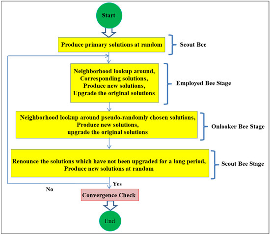
Figure 1. Flowchart of the Artificial Bee Colony (ABC).

3.2. Adaptive Neuro-Fuzzy Inference System (ANFIS)

ANFIS was first released by Jang [48]. The ANFIS integrates the features of artificial neural networks (ANN) and Fuzzy Inference Systems (FIS). Hence, it has quick learning capability, the potential of achieving the nonlinear framework of a system, and ability of adaptation. The quick learning capability is utilized for automatic fuzzy if-then principle generation and parameter optimization in ANFIS. Its inference system matches with a collection of fuzzy if-then principles which have learning capability to estimate nonlinear functions [48,49].

The ANFIS has been effectively applied to a wide range of issues in many different matters such as finance, accounting, financial engineering, economics, and management in ways that various objectives which includes analysis, assessment, and forecasting. The use of ANFIS for high-frequency data trading is highly effective.

ANFIS Structure

The ANFIS could solve any type of complex and nonlinear issue successfully by integrating the benefits of the ANN and FIS, and it leads to fewer errors. The structure of ANFIS is displayed in Figure 2. The ANFIS is basically the rule-based fuzzy modeling. Two rules which have employed in this structure are stated below:

$$\begin{gathered} R_1=\mathrm{If}x\mathrm{is}{A}_1\mathrm{and}y\mathrm{is}{B}_1\mathrm{Then}{f}_1=\left(p_{1}x+q_{1}y+r_1\right) \\ {R}_2=\mathrm{If}x \mathrm{is}{A}_2 \mathrm{and}y\mathrm{is}{B}_2\mathrm{Then}{f}_2=\left(p_{2}x+q_{2}y+r_2\right) \end{gathered}$$

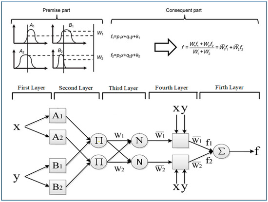
Figure 2. Adaptive Neuro-Fuzzy Interference System (ANFIS) Structure.

Wherein:

$A_1, B_1, A_2, B_2$: Membership functions of each input x and y

$p_1, p_2, q_1, q_2, r_1, r_2$: Linear parameters in part-Then (consequent part)

As shown in Figure 2, the ANFIS structure has five layers that the formulas of the layers are defined in Equations (5)–(12).

Layer 1:

$${\mu }_{Ai}(x)=exp\left[-{\left(\frac{x-c_i}{2a_i}\right)}^2\right]$$

(5)

$${\mu }_{Ai}(x)=\frac{1}{1+{\left|\frac{x-c_i}{a_i}\right|}^{2b}}$$

(6)

$$O_{1,i}={\mu }_{Ai}\left(x\right), i=1, 2$$

(7)

$$O_{1,i}={\mu }_{Bi-2} \left(y\right), i=3, 4$$

(8)

Layer 2:

$$O_{2,i}={\mu }_{Ai} \left(x\right)\ast {\mu }_{Bi} \left(y\right) i=1, 2$$

(9)

Layer 3:

$$O_{3,i}={\overline{w}}_i=\frac{w_i}{{{\displaystyle \sum }}_i{w}_i}V$$

(10)

Layer 4:

$$O_{4,i}={\overline{w}}_i{f}_i={\overline{w}}_i\left(p_{i}x+q_{i}y+r_i\right)$$

(11)

${\overline{w}}_i$: The normalized firing power from the previous layer

$\left(p_{i}x+q_{i}y+r_i\right)$: A parameter in the node

Layer 5:

$$O_{5,i}={\displaystyle \sum }_i{\overline{w}}_i{f}_i=\frac{{{\displaystyle \sum }}_i{w}_i{f}_i}{{{\displaystyle \sum }}_i{w}_i}$$

(12)

3.3. Support Vector Machine (SVM)

SVM is a learning machine applying structural risk and minimizing inductive principle to get beneficial generalization on a restricted number of learning patterns. Firstly, SVM has been released by Vapnik [50] and it is a learning program utilizing a high dimensional feature space.

SVM executes a learning algorithm and it is beneficial for identifying delicate patterns in complicated information collections. This algorithm runs discriminative category learning by instance to forecast the categories of earlier unobserved information. Figure 3 illustrates the SVM structure.

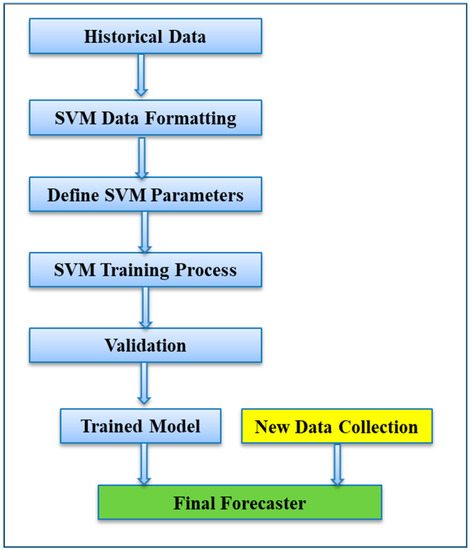
Figure 3. Support Vector Machine (SVM) Structure.

SVM evolved from studies in statistical learning theory on how to adjust generalization, and discover an optimum trade-off between structural intricacy and empirical risk.

SVM categorize points by allocating them to one of two disjoint half areas, either in the pattern area or in a higher-dimensional characteristic area [51,52]. The equation of standard SVM as follows:

$$f\left(x\right)=w_{x_i}^T+b=(w_1{x}_1+w_2{x}_2+w_3{x}_3+\cdots +w_n{x}_n+b)$$

(13)

Considering the f(x), the classification is obtained as:

$$\widehat{Y}=sign\left(f\left(x\right)\right)=\{\begin{array}{c}+1 f\left(x\right)>0\\ -1 f\left(x\right)<0\end{array}$$

(14)

Considering a linearly separable data-collection, the role of learning coefficients $w$ and $b$ of $f\left(x\right)=\left(w_{x_i}^T+b\right)$ decreases to fixing the following constrained optimization issue:

Find w and b that minimize: $\frac{1}{2}\Vert w^2\Vert$

Subject to constraints: $y_i=\left(w_{x_i}^T+b\right)\ge 1, \forall i$

This optimization issue could be fixed by applying the Lagrangian function determined as:

$$L \left(w,b,\alpha \right)=\frac{1}{2}{W}^{T}W-{\displaystyle \sum }_{i=1}^N\alpha i\left[y_i\left(w_{x_i}^T+b\right)-1\right]$$

(15)

$$\alpha i\ge 0 , \forall i$$

$$\alpha i\left[y_i\left(w_{x_i}^T+b\right)-1\right]=0, \forall i$$

(16)

Wherein ${\alpha }_1$,${\alpha }_2$, … ${\alpha }_N$ are Lagrange multipliers and $\alpha$ = [${\alpha }_1$,${\alpha }_2$, … ${\alpha }_N$]^T.

The answer of original limited optimization issue is specified by the saddle point of $L\left(w,b,\alpha \right)$ that has to be minimized with regards to $w$ and $b$ and maximized with regards to $\alpha$.

Consider the following about Lagrange multipliers:

• If $(w^T{x}_i+b)>1$, the value of ${\alpha }_i$ that maximizes $L\left(w,b,\alpha \right)$ is ${\alpha }_i$= 0.
• If $(w^T{x}_i+b)<1$, the value of ${\alpha }_i$ that maximizes $L\left(w,b,\alpha \right)$ is ${\alpha }_i$ = +∞.
• Considering that $w$ and $b$ are attempting to minimize $L$, they will be modified in such a way to make X at least equal to +1.

Data points $x_i$ with ${\alpha }_i$ > 0 are known as the support vectors.

3.3.1. Optimality Conditions

The essential statuses for the saddle point of L (w, b, α) are:

$$\frac{\partial L}{\partial W_j}=0, \forall j$$

$$\frac{\partial L}{\partial a_i}=0, \forall j$$

Or expressed $\alpha$ several procedures, ${\nabla }_{w}L=0, {\nabla }_{a}L=0$

Solving for the essential conditions leads to:

$$w={\displaystyle \sum }_{i=1}^N{\alpha }_i y_i x_i$$

(17)

$${\displaystyle \sum }_{i=1}^N{\alpha }_i y_i=0$$

(18)

By changing $w={\displaystyle \sum }_{i=1}^N{\alpha }_i y_i x_i$ into the Lagrangian function and by applying ${\displaystyle \sum }_{i=1}^N{\alpha }_i y_i=0$ as a new limitation, the dual optimization issue could be designed as follow:

Find α that maximizes: ${\displaystyle \sum }_{i=1}^N{\alpha }_i-\frac{1}{2} {\displaystyle \sum }_{i=1}^N{\displaystyle \sum }_{i=1}^N{\alpha }_i {\alpha }_j y_i y_{j }{X}_i^T{X}_j$

$\mathrm{Subject}\mathrm{to}: {\displaystyle {\displaystyle \sum }_{i=1}^N}{\alpha }_i{y}_i=0, {\alpha }_i\ge 0, \forall i$

3.3.2. Final Forecaster

Since the values ${\alpha }_1$, ${\alpha }_2$, … ${\alpha }_N$ acquired by the answer of the dual issue, the final SVM forecaster could be given from Equation (17) as:

$$f\left(x\right)=W^T{X}_i={\displaystyle \sum }_{i=1}^N{\alpha }_j y_i X_i^{T}X+b$$

(19)

Wherein:

$$b=\frac{1}{\left|I_{support}\right|}{{\displaystyle \sum }}_{i\in I_{support}}^N(y_i-{{\displaystyle \sum }}_{j=1}^N{\alpha }_j y_j X_j^T{X}_i)$$

(20)

$I_{support}$: The set of support vectors.

We consider the following about support vectors:

• Given that ${\alpha }_i$ ≠ 0 merely for the support vectors, just support vectors are employed in achieving to forecasting model.
• Notice that $x_j^T{x}_i$ is a scalar.

3.4. Technical Indicators

Technical indicators are concentrated on historical information, for instance, price and volume, instead of the fundamental analysis of the trade. There are plenty of indicators in the market that can be utilized to reveal the momentum, trend, volatility, etc., and they are based on mathematical equations, which are the interpreters of the market. They check out price data and convert it into easy and useful signals which can assist investors and traders to specify when to buy or sell. Any technical indicator presents exclusive data and check out historical price information. They could be utilized as numerous indicators in combination with other indicators.

After the review of the past studies and related papers, we selected twenty original technical indicators that have major roles in the technical analysis and stock price forecasting. These technical indicators, which are listed in Table 1, could cover all stock data by considering the four classes including Oscillator, Index, Overlay, and Cumulative. Based on previous researches and viewpoints of technical experts and professionals, the twenty chosen technical indicators are the most essential indicators in the technical analysis.

Table 1. List of Selected Technical Indicators.

No.	Indicator	Type	Class
1	Absolute Price Oscillator (APO)	Trend	Oscillator
2	Accumulation Distribution (AD)	Volume	Cumulative
3	Average Directional Movement (ADX)	Trend	Index
4	Average True Range (ATR)	Volatility	Index
5	Bollinger Bands (BBANDS)	Volatility	Overlay
6	Chande Momentum Oscillator (CMO)	Momentum	Oscillator
7	Commodity Channel Index (CCI)	Momentum	Oscillator
8	Directional Movement Index (DMI)	Trend	Index
9	Fast Stochastic	Momentum	Oscillator
10	Fibonacci Arc	Support and Resistance	Overlay
11	Fibonacci Fan	Support and Resistance	Overlay
12	Fibonacci Retracement	Support and Resistance	Overlay
13	Fibonacci Time Zones	Support and Resistance	Overlay
14	Moving Average Convergence Divergence (MACD)	Trend	Oscillator
15	On Balance Volume (OBV)	Volume	Cumulative
16	Parabolic Stop and Reverse (SAR)	Trend	Overlay
17	Rate of Change (ROC)	Momentum	Oscillator
18	Relative Strength Index (RSI)	Momentum	Oscillator
19	Volume Oscillator (VO)	Volume	Oscillator
20	Williams %R	Momentum	Oscillator

3.5. Proposed Model

Figure 4 illustrates the architecture of the presented model for the stock price forecasting. This figure shows that the ABC and ANFIS modules have been employed to multi-objective optimization of technical indicators, and the SVM module has been used to produce trading signals (Buy/Sale/Hold/Neutral).

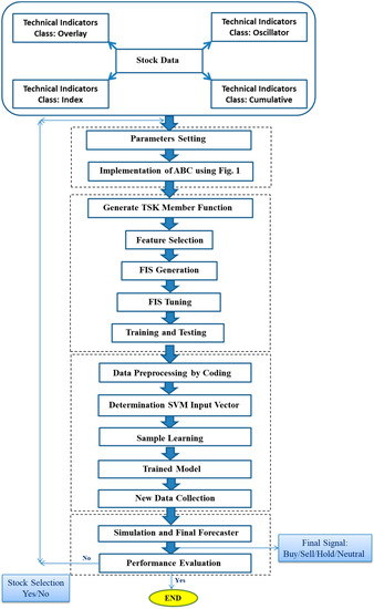
Figure 4. Proposed Model.

After the calculations of the technical indicators outlined in Table 1, they have been applied in the model as input variables. At the first stage, the ABC is applied to optimize the technical indicators for forecasting tools. At the second stage, the ANFIS is implemented to predict the future price of stocks. At the third stage, the SVM has been used to data preprocessing by coding and then the data have been normalized. The determination of the input vector and sample learning are the last phases of the SVM. Eventually, the final signal will be obtained from the model.

3.6. Data and Parameter Setting

We execute the ABC-ANFIS-SVM by applying the daily stock price of the 50 largest American companies on the stock market, which are listed in Table A1 (see Appendix A). All of the information is collected from www.nyse.com, www.nasdaq.com, and www.marketwatch.com.

The periods of our research are adequate for testing and validation of the model because the boom and bust cycle and the economic fluctuations and important political events have happened during the years 2008–2018. To increase accuracy and avoid mistakes, sample selection in the training and testing data is divided into five periods of two years.

The details about the training and testing data are provided in Table 2. Approximately 80% of the data was intended for training, and 20% for testing. Four parameters from the stock exchange are employed to create the vectors and explanations of the parameters are mentioned in Table 3.

Table 2. Training and Testing Data.

Training Data		Observations	Testing Data		Observations
From	To		From	To
31 Jan 2008	31 Dec 2009	544	31 Dec 2009	31 Dec 2010	136
31 Dec 2010	31 Dec 2011	636	31 Dec 2011	31 Dec 2012	159
31 Dec 2012	31 Dec 2013	704	31 Dec 2011	31 Dec 2014	176
31 Dec 2014	31 Dec 2015	832	31 Dec 2015	31 Dec 2016	208
31 Dec 2016	31 Dec 2017	996	31 Dec 2017	31 Dec 2018	249

Table 3. Parameter Explanation.

Parameter	Explanation
Open Price	The first stock price at the beginning of daily dealing
Close Price	The last stock price at the end of daily dealing
High Price	The maximum stock price at the during daily dealing
Low Price	The minimum stock price at the during daily dealing

The parameter adjustments are essential since they can have a negative impact on the model performance if they are not correctly regulated. The adjustments of parameters are detailed in Table 4 and Table 5. The best-suited adjustments are planned for comparison with the other methods.

Table 4. ABC Parameter Settings.

Parameter	Level
Swarm size	100
Limit	Number of onlooker bees
Number of Onlookers	50% of the swarm
Number of Employed Bees	50% of the swarm
Number of Scouts	1
Maximum Cycle	3000

Table 5. SVM Parameter Settings.

Parameter	Level
Degree of kernel function	1, 2, 3, 4
Gamma in kernel function	0, 0.1, 0.2, …, 5
Regularization parameter	1, 10, 100

The technical indicators are the input variables and the output objectives are stock’s future price and the signals for buy/hold/sell.

4. Results and Evaluation

In this section, we evaluate the performance of the offered model and compare it with the other approaches. To enhance the credibility of the proposed model, five criteria for accuracy and quality are evaluated. These criteria determine the deviation between observed and forecasted values. These measures include RMSE, MAE, MAPE, and Theil’s U (U₁, U₂) and the formulas for them are as follows:

$$RMSE=\sqrt{\frac{1}{N}{\displaystyle \sum }_{t=1}^N{\left(O_t-F_t\right)}^2}$$

(21)

$$MAE=\frac{1}{N} {\displaystyle \sum }_{t=1}^N\left|O_t-F_t\right|$$

(22)

$$MAPE=\frac{1}{N} {\displaystyle \sum }_{t=1}^N\left|\frac{O_t-F_t}{O_t}\right|$$

(23)

$$Theil’s U_1=\frac{{\left[{{\displaystyle \sum }}_{t=1}^N{\left(O_t-F_t\right)}^2\right]}^{\frac{1}{2}}}{{\left[{{\displaystyle \sum }}_{t=1}^N{F}_t{}^2\right]}^{\frac{1}{2}}}$$

(24)

$$Theil’s U_2=\frac{{\left[\frac{1}{N} {{\displaystyle \sum }}_{t=1}^N{\left(O_t-F_t\right)}^2\right]}^{\frac{1}{2}}}{{\left[\frac{1}{N}{{\displaystyle \sum }}_{t=1}^N{O}_t{}^2\right]}^{\frac{1}{2}}+{\left[\frac{1}{N}{{\displaystyle \sum }}_{t=1}^N{F}_t{}^2\right]}^{\frac{1}{2}}}$$

(25)

Wherein $O_t$ indicates the observed price and $F_t$ shows the forecasted price at time t.

Theil suggested two U statistics contains U₁ and U₂, employed in finance. The U₁ is a criterion of prediction accuracy [53]. The U₂ is a criterion of prediction quality [54]. The interpretation of the Theil’s U is mentioned in Table A2 (see Appendix A).

The comparison outcomes of three key indexes in the U.S. Stock Exchange are shown in Table 6, Table 7, Table 8, Table 9 and Table 10, which prove that our technique has increased the forecasting precision and quality for all the three indexes.

Table 6. The outcomes of key indexes (U.S. SE) in terms of RMSE.

RMSE
	2008	2009	2010	2011	2012	2013	2014	2015	2016	2017	2018
DOW 30	1.9635	1.7415	1.2588	1.0072	0.9152	0.8253	0.8145	0.7495	0.6824	0.1374	0.1072
NASDAQ 100	1.8405	1.8673	1.4568	1.2475	0.9314	0.9652	0.8752	0.7510	0.6725	0.1049	0.0641
S&P 500	1.7251	1.7425	1.5325	1.3247	0.9254	0.0844	0.7484	0.7155	0.6649	0.0458	0.0367

Table 7. The outcomes of key indexes (U.S. SE) in terms of MAE.

MAE
	2008	2009	2010	2011	2012	2013	2014	2015	2016	2017	2018
DOW 30	0.0086	0.0074	0.0153	0.0110	0.0244	0.0169	0.0281	0.0352	0.0324	0.0172	0.0158
NASDAQ 100	0.0125	0.0145	0.0421	0.0472	0.0296	0.0231	0.0327	0.0043	0.0441	0.0255	0.0241
S&P 500	0.0837	0.0210	0.0168	0.0088	0.0072	0.0053	0.0345	0.0114	0.0147	0.0125	0.0014

Table 8. The outcomes of key indexes (U.S. SE) in terms of MAPE.

MAPE (%)
	2008	2009	2010	2011	2012	2013	2014	2015	2016	2017	2018
DOW 30	0.8642	0.7435	0.6941	0.5638	0.4825	0.3476	0.2724	0.1586	0.1435	0.1325	0.1272
NASDAQ 100	0.8125	0.7158	0.6547	0.5418	0.4274	0.3595	0.2643	0.1614	0.1496	0.1359	0.1324
S&P 500	0.8847	0.7856	0.6214	0.5169	0.4532	0.3751	0.2785	0.1695	0.1524	0.1363	0.1398

Table 9. The outcomes of key indexes (U.S. SE) in terms of U_1.

U1
	2008	2009	2010	2011	2012	2013	2014	2015	2016	2017	2018
DOW 30	0.0092	0.0086	0.0082	0.0075	0.0069	0.0067	0.0062	0.0059	0.0042	0.0031	0.0014
NASDAQ 100	0.0201	0.0115	0.0147	0.0224	0.0077	0.0069	0.0056	0.0048	0.0037	0.0024	0.0018
S&P 500	0.0152	0.0097	0.0131	0.0083	0.0081	0.0074	0.0069	0.0051	0.0044	0.0038	0.0023

Table 10. The outcomes of key indexes (U.S. SE) in terms of U_2.

U2
	2008	2009	2010	2011	2012	2013	2014	2015	2016	2017	2018
DOW 30	0.0128	0.0141	0.0124	0.0109	0.0083	0.0081	0.0066	0.0052	0.0041	0.0028	0.0017
NASDAQ 100	0.0173	0.0155	0.0147	0.0136	0.0112	0.0092	0.0071	0.0046	0.0065	0.0033	0.0021
S&P 500	0.0169	0.0165	0.0162	0.0141	0.0101	0.0095	0.0079	0.0075	0.0054	0.0037	0.0025

To validation the model, the final results have been revealed in Table 6, Table 7, Table 8, Table 9, Table 10 and Table 11. According to the outcomes in these tables, it can be observed that the ABC-ANFIS-SVM could provide the lowest error and the topmost accuracy under the testing model.

Table 11. The final outcomes of the model in comparison with other methods.

Method	RMSE	MAE	MAPE (%)	U1	U2
ABC-ANFIS-SVM	0.0092	0.0088	0.7283	0.0012	0.0009
ARIMA-SVM	1.0021	0.0142	2.3769	0.0489	0.0324
ABC-SVM	0.8864	0.0098	1.8237	0.0272	0.0256
ABC-ANFIS	0.9235	0.0095	1.2920	0.0195	0.0144
ANFIS-SVM	1.8934	0.0117	0.9436	0.0121	0.0132
ARIMA-ANFIS	1.1473	0.0182	2.9124	0.1025	0.0763
WANFIS [46]	0.0378	0.0136	1.4515	0.0196	0.0056
SVM [45]	0.0276	0.0129	0.9307	0.0021	0.0049
QGGABC-FFNN [44]	0.0635	0.0155	1.1250	0.1036	0.0042
ANN-SVM [39]	0.0414	0.0372	0.8403	0.1128	0.0053
HWT-ANN-DABC [38]	0.0526	0.0436	1.4937	0.0255	0.0071
FA-MSVR [36]	0.0387	0.0130	1.0533	0.1072	0.0178
PSO-SVM [35]	0.0443	0.0227	1.1714	0.1369	0.0144
GA-ANFIS [34]	0.0725	0.0316	0.9325	0.0141	0.0058
ANFIS [33]	0.0847	0.0407	1.2746	0.0095	0.0082
ANN-SVM [32]	0.0481	0.0521	1.0255	0.0122	0.0039
NN-SVR [28]	0.0532	0.0368	1.0367	0.0086	0.0052
SOFM-SVR [24]	0.0654	0.0445	0.9366	0.0074	0.0095
KPCA-SVR [23]	0.0793	0.0504	0.8941	0.0098	0.0077
ARIMA-ANN-SVM [20]	0.0449	0.0172	0.8452	0.0059	0.0086
SVM-RF [18]	0.0172	0.0245	1.3417	0.0132	0.0047

Table 11 indicates that the RMSE, MAE, and MAPE for the ABC-ANFIS-SVM are less than the other models. Moreover, U₁ and U₂ for our method are higher than the other methods.

When implementing ANFIS the articles cited in the references were used [55,56]. All of the methods have been executed in “Mathworks MATLAB R2019” software. All in all, according to RMSE, MAE, MAPE, U₁, and U₂ criteria, we derived that ABC-ANFIS-SVM functions best in terms of accuracy and quality. The ABC-ANFIS-SVM is evaluated to other methods which are proved by five criteria. All values of our model are higher than other methods for all indices. For SVM implementations, all tests were executed on “Mathworks MATLAB” software utilizing LIBSVM [57].

The actual values and forecasted values for ABC-ANFIS-SVM are displayed in Figure 5, Figure 6, Figure 7, Figure 8, Figure 9, Figure 10 and Figure 11. The blue points represent forecasted values and the red lines represent observed values.

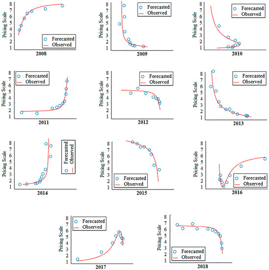
Figure 5. Samples of forecasted and observed prices for each year.

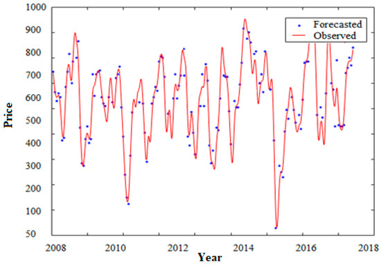
Figure 6. Performance Evaluation of ABC-ANFIS-SVM.

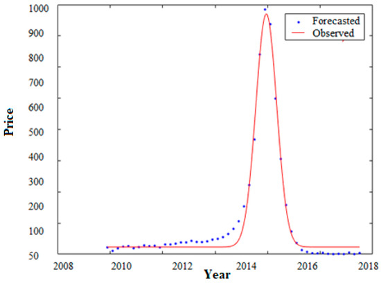
Figure 7. Model Fit (Training Data).

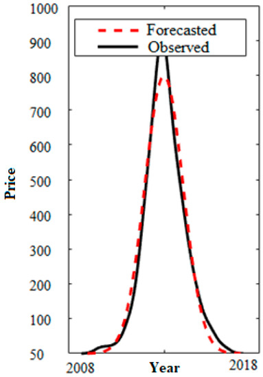
Figure 8. Model Fit (Testing Data).

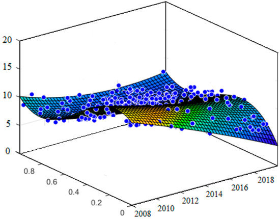
Figure 9. Model Matching Results (No. 1).

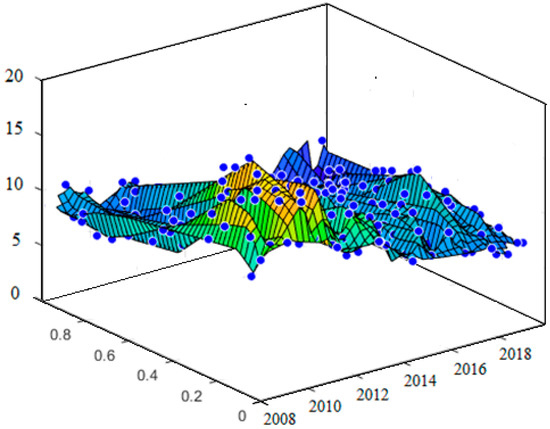
Figure 10. Model Matching Results (No. 2).

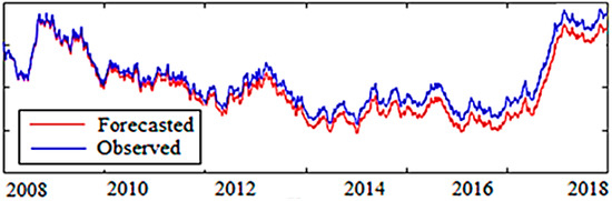
Figure 11. Model Testing Results

The functionality for every year is computed and the outcomes have been displayed in Figure 5. Figure 6 illustrates the performance evaluation of ABC-ANFIS-SVM that corroborates the best performance. The forecasted prices approximately correspond with the trend of the observed prices.

Figure 7 and Figure 8 indicate the model performance for both training data and testing data which confirmed that our model is a prosperous tool for stock price forecasting. The results of the testing model and model matching are displayed in Figure 9, Figure 10 and Figure 11 which are so satisfactory and adequate.

Table 12, Table 13, Table 14, Table 15, Table 16, Table 17, Table 18, Table 19, Table 20, Table 21, Table 22 and Table 23 show the final signals of ABC-ANFIS-SVM model, which will offer trading signals to investors and financial analysts after calculating technical indicators and accurate stock price forecasts. These tables are provided as examples for the 12 largest American companies for the validation and verification of the presented model. Consequently, all the signals are approved according to the period of a particular transaction.

Table 12. The final signal obtained from ABC-ANFIS-SVM (Example 1).

Microsoft Corp
Indicator	Value	Signal
RSI	82.763	Overbought
STOCH	72.536	Buy
STOCHRSI	101.000	Overbought
MACD	0.671	Buy
ADX	43.619	Buy
Williams %R	−3.778	Overbought
CCI	145.277	Buy
ATR	0.6043	High Volatility
Highs/Lows	1.254	Buy
Ultimate Oscillator	62.808	Buy
ROC	2.142	Buy
Bull/Bear Power	2.035	Buy

Note: Buy: 8; Sell: 0; Neutral: 0; Final Signal: Strong Buy.

Table 13. The final signal obtained from ABC-ANFIS-SVM (Example 2).

Exxon Mobil
Indicator	Value	Signal
RSI	40.631	Sell
STOCH	35.256	Sell
STOCHRSI	0.000	Oversold
MACD	−0.020	Sell
ADX	51.807	Buy
Williams %R	−92.659	Oversold
CCI	−128.731	Sell
ATR	0.346	High Volatility
Highs/Lows	−0.185	Sell
Ultimate Oscillator	52.112	Buy
ROC	−0.114	Sell
Bull/Bear Power	−0.0600	Sell

Note: Buy: 2; Sell: 7; Neutral: 0; Final Signal: Strong Sell.

Table 14. The final signal obtained from ABC-ANFIS-SVM (Example 3).

BHP Group PLC
Indicator	Value	Signal
RSI	44.272	Neutral
STOCH	73.881	Buy
STOCHRSI	92.153	Overbought
MACD	−7.042	Sell
ADX	37.850	Buy
Williams %R	−23.489	Buy
CCI	83.704	Buy
ATR	7.258	Less Volatility
Highs/Lows	2.965	Buy
Ultimate Oscillator	59.423	Buy
ROC	0.462	Buy
Bull/Bear Power	−1.257	Sell

Note: Buy: 7; Sell: 2; Neutral: 1; Final Signal: Strong Buy.

Table 15. The final signal obtained from ABC-ANFIS-SVM (Example 4).

Walmart Inc
Indicator	Value	Signal
RSI	57.117	Buy
STOCH	45.756	Neutral
STOCHRSI	0.020	Oversold
MACD	0.541	Buy
ADX	14.236	Neutral
Williams %R	−46.287	Neutral
CCI	55.763	Buy
ATR	0.404	Less Volatility
Highs/Lows	0.005	Neutral
Ultimate Oscillator	47.624	Sell
ROC	0.345	Buy
Bull/Bear Power	0.372	Buy

Note: Buy: 5; Sell: 1; Neutral: 4; Final Signal: Strong Buy.

Table 16. The final signal obtained from ABC-ANFIS-SVM (Example 5).

Apple Inc
Indicator	Value	Signal
RSI	72.445	Buy
STOCH	80.078	Overbought
STOCHRSI	91.363	Overbought
MACD	1.202	Buy
ADX	54.495	Buy
Williams %R	−7.114	Overbought
CCI	99.103	Buy
ATR	1.605	Less Volatility
Highs/Lows	0.712	Buy
Ultimate Oscillator	55.762	Buy
ROC	2.225	Buy
Bull/Bear Power	2.189	Buy

Note: Buy: 8; Sell: 0; Neutral: 0; Final Signal: Strong Buy.

Table 17. The final signal obtained from ABC-ANFIS-SVM (Example 6).

Facebook Inc
Indicator	Value	Signal
RSI	51.247	Buy
STOCH	42.320	Neutral
STOCHRSI	8.673	Oversold
MACD	0.299	Buy
ADX	33.412	Sell
Williams %R	−40.350	Buy
CCI	43.931	Neutral
ATR	0.520	Less Volatility
Highs/Lows	0.001	Neutral
Ultimate Oscillator	51.715	Buy
ROC	−0.482	Sell
Bull/Bear Power	0.325	Buy

Note: Buy: 5; Sell: 2; Neutral: 3; Final Signal: Buy.

Table 18. The final signal obtained from ABC-ANFIS-SVM (Example 7).

Amazon Inc
Indicator	Value	Signal
RSI	58.431	Buy
STOCH	51.572	Neutral
STOCHRSI	43.215	Sell
MACD	1.507	Buy
ADX	32.725	Buy
Williams %R	−39.439	Buy
CCI	69.247	Buy
ATR	3.234	Less Volatility
Highs/Lows	0.005	Neutral
Ultimate Oscillator	51.734	Buy
ROC	−0.080	Sell
Bull/Bear Power	3.933	Buy

Note: Buy: 7; Sell: 2; Neutral: 2; Final Signal: Strong Buy.

Table 19. The final signal obtained from ABC-ANFIS-SVM (Example 8).

General Electric Co.
Indicator	Value	Signal
RSI	64.423	Buy
STOCH	60.363	Buy
STOCHRSI	100.000	Overbought
MACD	0.060	Buy
ADX	53.721	Buy
Williams %R	0.000	Overbought
CCI	199.423	Overbought
ATR	0.073	Less Volatility
Highs/Lows	0.157	Buy
Ultimate Oscillator	65.176	Buy
ROC	2.349	Buy
Bull/Bear Power	0.301	Buy

Note: Buy: 8; Sell: 0; Neutral: 0; Final Signal: Strong Buy.

Table 20. The final signal obtained from ABC-ANFIS-SVM (Example 9).

Intel Corp
Indicator	Value	Signal
RSI	66.472	Buy
STOCH	60.356	Buy
STOCHRSI	11.225	Oversold
MACD	6.078	Buy
ADX	29.523	Buy
Williams %R	−31.782	Buy
CCI	42.860	Neutral
ATR	6.107	Less Volatility
Highs/Lows	0.006	Neutral
Ultimate Oscillator	49.041	Neutral
ROC	0.906	Buy
Bull/Bear Power	1.923	Buy

Note: Buy: 7; Sell: 0; Neutral: 3; Final Signal: Strong Buy.

Table 21. The final signal obtained from ABC-ANFIS-SVM (Example 10).

Chevron Corp
Indicator	Value	Signal
RSI	40.965	Sell
STOCH	63.746	Buy
STOCHRSI	100.000	Overbought
MACD	−0.907	Sell
ADX	25.058	Sell
Williams %R	−28.655	Buy
CCI	30.627	Neutral
ATR	1.736	Less Volatility
Highs/Lows	0.0812	Buy
Ultimate Oscillator	55.311	Buy
ROC	−4.073	Sell
Bull/Bear Power	−0.665	Sell

Note: Buy: 4; Sell: 5; Neutral: 1; Final Signal: Sell.

Table 22. The final signal obtained from ABC-ANFIS-SVM (Example 11).

Bank of America Corp
Indicator	Value	Signal
RSI	49.352	Neutral
STOCH	55.964	Buy
STOCHRSI	26.398	Sell
MACD	0.019	Buy
ADX	23.120	Buy
Williams %R	−50.342	Neutral
CCI	−33.156	Neutral
ATR	0.0834	Less Volatility
Highs/Lows	0.009	Neutral
Ultimate Oscillator	50.057	Neutral
ROC	−1.385	Sell
Bull/Bear Power	−0.013	Sell

Note: Buy: 3; Sell: 2; Neutral: 5; Final Signal: Neutral.

Table 23. The final signal obtained from ABC-ANFIS-SVM (Example 12).

Nike Inc
Indicator	Value	Signal
RSI	49.632	Neutral
STOCH	57.925	Buy
STOCHRSI	25.302	Sell
MACD	0.014	Buy
ADX	20.072	Buy
Williams %R	−55.631	Neutral
CCI	−31.305	Neutral
ATR	0.081	Less Volatility
Highs/Lows	0.009	Neutral
Ultimate Oscillator	51.204	Neutral
ROC	−1.627	Sell
Bull/Bear Power	−0.0107	Sell

Note: Buy: 3; Sell: 3; Neutral: 5; Final Signal: Neutral.

5. Conclusions

In this paper, a new approach for the stock price forecasting was created by integrating ABC, ANFIS, and SVM to more precisely predict the stock prices. Forecasting the trends of activities of the stock price is crucial for the progress of efficient investment policies. In this investigation, we have integrated the ABC-ANFIS into the SVM forecasting model to optimize the technical indicators. We have tried with ABC-ANFIS-SVM to achieve an approximation of the topmost attainable accuracy and quality for stock price forecasting. With the purpose to analyze the ABC-ANFIS-SVM, we employed it on stock price data of the U.S. Stock Exchange from 2008 to 2018, which has been applied as the case study. Twenty technical indicators were employed in our model as input variables.

To display the functionality and superiority of the model, five criteria were examined. After examining the experimental results, we unmistakably have noticed that the presented approach is designed to simulate the active unpredictable stock markets efficiently, which produces a more accurate and high-quality model as compared with other methods. It is obvious that the outcomes authenticate that the novel approach substantially boosts the reliability of the ABC-ANFIS-SVM model. In fact, our approach is the first hybrid model that combines three modules ABC, ANFIS, and SVM together with performance evaluation by the criteria of accuracy and quality. It implies that the model has lesser diversions between forecasted and observed prices than the other methods. Furthermore, the output signals confirmed that the twenty selected technical indicators were absolutely appropriate and comprehensive. The key advantages of our model include enhancing speed and precision in computation, reaching the most optimal technical indicators and the ability to obtain an active strategy to invest in the stock exchange and portfolio building. In future works, the presented model can be further studied by using other soft computing methods or by attaching other techniques or additional input variables. Additionally, the model can be employed for other financial markets.

The computational analysis has revealed that ABC-ANFIS-SVM is the most efficient approach for stock price forecasting and it could be employed in other challenges associated with financial predicting. From the point of view of the authors, the overall functionality of the presented model in the stock price forecasting works better than related studies in the previous investigations. Nevertheless, the function of our model may be developed by two ideas. Firstly, by setting the model parameters by running more sensitive and extensive variables adjustment, which can be subsequent articles for research workers. Secondly, the supplementary or alternative variables can be used as inputs of the model, for instance: foreign exchange rates, interest rates, and many others.

According to the results of the model evaluation and its performance, we conclude that the investigation aims have been achieved. Even so, we are encountered with two limitations about forces that move stock prices. Besides the technical factors, there are two other important factors that can affect stock prices: (1) Fundamental factors and (2) market sentiment. Our model can be improved considerably by taking into account these two items. In our future work, we intend to take into account these items and will present a newer model.

The unique attributes of this work:

• Proposing a novel efficient hybrid model based on ABC, ANFIS, and SVM
• Applying the comprehensive and major technical indicators
• Multi-objective optimization of technical indicators

Ultimately, we summarize the key outcomes of the article in the following cases:

• This study indicates that the challenge of stock price forecasting can be solved by employing ABC-ANFIS-SVM.
• This study indicates that the forecasting accuracy and reliability of the ABC-ANFIS-SVM is more accurate than the other models.
• This study indicates the strength of the ABC-ANFIS-SVM model by comparing its predicting quality with different methods.

References

- Tsang, P.M.; Kwok, P.; Choy, S.O.; Kwan, R.; Ng, S.C.; Mak, J.; Tsang, J.; Koong, K.; Wong, T.L. Design and implementation of NN5 for Hong Kong stock price forecasting. Eng. Appl. Artif. Intell. 2007, 20, 453–461. [Google Scholar] [CrossRef]
- Ritchie, J.C. Fundamental Analysis: A Back-to-the-Basics Investment Guide to Selecting Quality Stocks; Irwin Professional Pub: Burr Ridge, IL, USA, 1996. [Google Scholar]
- Murphy, J.J. Technical Analysis of the Financial Markets: A Comprehensive Guide to Trading Methods and Applications; Penguin: London, UK, 1999. [Google Scholar]
- Box, G.E.; Jenkins, G.M. Time Series Analysis: Forecasting and Control San Francisco; Holden-Day: San Francisco, CA, USA, 1976. [Google Scholar]
- Karaboga, D.; Basturk, B. On the performance of artificial bee colony (ABC) algorithm. Appl. Soft Comput. 2008, 8, 687–697. [Google Scholar] [CrossRef]
- Kim, J.; Kasabov, N. HyFIS: Adaptive neuro-fuzzy inference systems and their application to nonlinear dynamical systems. Neural Netw. 1999, 12, 1301–1319. [Google Scholar] [CrossRef]
- Sharma, M.; Sharma, S.; Singh, G. Performance Analysis of Statistical and Supervised Learning Techniques in Stock Data Mining. Data 2018, 3, 54. [Google Scholar] [CrossRef]
- Chapelle, O.; Vapnik, V.; Bousquet, O.; Mukherjee, S. Choosing multiple parameters for support vector machines. Mach. Learn. 2002, 46, 131–159. [Google Scholar] [CrossRef]
- Kimoto, T.; Asakawa, K.; Yoda, M.; Takeoka, M. Stock market prediction system with modular neural networks. In Proceedings of the 1990 IJCNN International Joint Conference on Neural Networks, San Diego, CA, USA, 17–21 June 1990; pp. 1–6. [Google Scholar]
- Kamijo, K.-I.; Tanigawa, T. Stock price pattern recognition-a recurrent neural network approach. In Proceedings of the 1990 IJCNN International Joint Conference on Neural Networks, San Diego, CA, USA, 17–21 June 1990; pp. 215–221. [Google Scholar]
- Yoon, Y.; Swales, G. Predicting stock price performance: A neural network approach. In Proceedings of the Twenty-Fourth Annual Hawaii International Conference on System Sciences, Kauai, HI, USA, 8–11 January 1991; pp. 156–162. [Google Scholar]
- Baba, N.; Kozaki, M. An intelligent forecasting system of stock price using neural networks. In Proceedings of the 1992 IJCNN International Joint Conference on Neural Networks, Baltimore, MD, USA, 7–11 June 1992; pp. 371–377. [Google Scholar]
- Cheung, Y.-M.; Lai, H.Z.; Xu, L. Application of adaptive RPCL-CLP with trading system to foreign exchange investment. In Proceedings of the International Conference on Neural Networks (ICNN’96), Washington, DC, USA, 3–6 June 1996; pp. 131–136. [Google Scholar]
- Saad, E.W.; Prokhorov, D.V.; Wunsch, D.C. Comparative study of stock trend prediction using time delay, recurrent and probabilistic neural networks. IEEE Trans. Neural Netw. 1998, 9, 1456–1470. [Google Scholar] [CrossRef]
- Takahashi, T.; Tamada, R.; Nagasaka, K. Multiple line-segments regression for stock prices and long-range forecasting system by neural network. In Proceedings of the 37th SICE Annual Conference. International Session Papers, Chiba, Japan, 29–31 July 1998; pp. 1127–1132. [Google Scholar]
- Kim, K.-J. Financial time series forecasting using support vector machines. Neurocomputing 2003, 55, 307–319. [Google Scholar] [CrossRef]
- Pai, P.-F.; Lin, C.-S. A hybrid ARIMA and support vector machines model in stock price forecasting. Omega 2005, 33, 497–505. [Google Scholar] [CrossRef]
- Manish, K.; Thenmozhi, M. Forecasting stock index movement: A comparison of support vector machines and random forest. In Proceedings of the Ninth Indian Institute of Capital Markets Conference, Mumbai, India, 19–20 December 2005. [Google Scholar]
- Huang, W.; Nakamori, Y.; Wang, S.-Y. Forecasting stock market movement direction with support vector machine. Comput. Oper. Res. 2005, 32, 2513–2522. [Google Scholar] [CrossRef]
- Kumar, M.; Thenmozhi, M. Support vector machines approach to predict the S&P CNX NIFTY index returns. SSRN Electron. J. 2007. [Google Scholar] [CrossRef]
- Chang, P.-C.; Liu, C.-H. A TSK type fuzzy rule based system for stock price prediction. Expert Syst. Appl. 2008, 34, 135–144. [Google Scholar] [CrossRef]
- Ince, H.; Trafalis, T.B. Short term forecasting with support vector machines and application to stock price prediction. Int. J. Gen. Syst. 2008, 37, 677–687. [Google Scholar] [CrossRef]
- Huang, C.-L.; Tsai, C.-Y. A hybrid SOFM-SVR with a filter-based feature selection for stock market forecasting. Expert Syst. Appl. 2009, 36, 1529–1539. [Google Scholar] [CrossRef]
- Hsu, S.-H.; Hsieh, J.P.-A.; Chih, T.-C.; Hsu, K.-C. A two-stage architecture for stock price forecasting by integrating self-organizing map and support vector regression. Expert Syst. Appl. 2009, 36, 7947–7951. [Google Scholar] [CrossRef]
- Atsalakis, G.S.; Valavanis, K.P. Surveying stock market forecasting techniques–Part II: Soft computing methods. Expert Syst. Appl. 2009, 36, 5932–5941. [Google Scholar] [CrossRef]
- Atsalakis, G.S.; Valavanis, K.P. Surveying stock market forecasting techniques-Part I: Conventional methods. J. Comput. Optim. Econ. Financ. 2010, 2, 45–92. [Google Scholar]
- Liang, X.; Zhang, H.; Xiao, J.; Chen, Y. Improving option price forecasts with neural networks and support vector regressions. Neurocomputing 2009, 72, 3055–3065. [Google Scholar] [CrossRef]
- Hadavandi, E.; Shavandi, H.; Ghanbari, A. Integration of genetic fuzzy systems and artificial neural networks for stock price forecasting. Knowl. Based Syst. 2010, 23, 800–808. [Google Scholar] [CrossRef]
- Lu, C.-J. Integrating independent component analysis-based denoising scheme with neural network for stock price prediction. Expert Syst. Appl. 2010, 37, 7056–7064. [Google Scholar] [CrossRef]
- Cheng, C.-H.; Chen, T.-L.; Wei, L.-Y. A hybrid model based on rough sets theory and genetic algorithms for stock price forecasting. Inf. Sci. 2010, 180, 1610–1629. [Google Scholar] [CrossRef]
- Kara, Y.; Boyacioglu, M.A.; Baykan, Ö.K. Predicting direction of stock price index movement using artificial neural networks and support vector machines: The sample of the Istanbul Stock Exchange. Expert Syst. Appl. 2011, 38, 5311–5319. [Google Scholar] [CrossRef]
- Svalina, I.; Galzina, V.; Lujić, R.; ŠImunović, G. An adaptive network-based fuzzy inference system (ANFIS) for the forecasting: The case of close price indices. Expert Syst. Appl. 2013, 40, 6055–6063. [Google Scholar] [CrossRef]
- Wei, L.-Y. A hybrid model based on ANFIS and adaptive expectation genetic algorithm to forecast TAIEX. Econ. Model. 2013, 33, 893–899. [Google Scholar] [CrossRef]
- Chen, S.-M.; Kao, P.-Y. TAIEX forecasting based on fuzzy time series, particle swarm optimization techniques and support vector machines. Inf. Sci. 2013, 247, 62–71. [Google Scholar] [CrossRef]
- Xiong, T.; Bao, Y.; Hu, Z. Multiple-output support vector regression with a firefly algorithm for interval-valued stock price index forecasting. Knowl. Based Syst. 2014, 55, 87–100. [Google Scholar] [CrossRef]
- Hafezi, R.; Shahrabi, J.; Hadavandi, E. A bat-neural network multi-agent system (BNNMAS) for stock price prediction: Case study of DAX stock price. Appl. Soft Comput. 2015, 29, 196–210. [Google Scholar] [CrossRef]
- Khuat, T.T.; Le, Q.C.; Nguyen, B.L.; Le, M.H. Forecasting Stock Price using Wavelet Neural Network Optimized by Directed Artificial Bee Colony Algorithm. J. Telecommun. Inf. Technol. 2016, 2, 43–52. [Google Scholar]
- Pyo, S.; Lee, J.; Cha, M.; Jang, H. Predictability of machine learning techniques to forecast the trends of market index prices: Hypothesis testing for the Korean stock markets. PLoS ONE 2017, 12, e0188107. [Google Scholar] [CrossRef]
- Preethi, G.; Santhi, B. Stock Market Forecasting Techniques: A Survey. J. Theor. Appl. Inf. Technol. 2012, 46, 24–30. [Google Scholar]
- Zhang, L.; Aggarwal, C.; Qi, G.-J. Stock price prediction via discovering multi-frequency trading patterns. In Proceedings of the 23rd ACM SIGKDD International Conference on Knowledge Discovery and Data Mining, Halifax, NS, Canada, 13–17 August 2017; ACM: New York, NY, USA, 2017; pp. 2141–2149. [Google Scholar]
- Nguyen, N. An Analysis and Implementation of the Hidden Markov Model to Technology Stock Prediction. Risks 2017, 5, 62. [Google Scholar] [CrossRef]
- Nguyen, N. Hidden Markov Model for Stock Trading. Int. J. Financ. Stud. 2018, 6, 36. [Google Scholar] [CrossRef]
- Shah, H.; Tairan, N.; Garg, H.; Ghazali, R. A quick gbest guided artificial bee colony algorithm for stock market prices prediction. Symmetry 2018, 10, 292. [Google Scholar] [CrossRef]
- Dinh, T.-A.; Kwon, Y.-K. An empirical study on importance of modeling parameters and trading volume-based features in daily stock trading using neural networks. In Informatics; Multidisciplinary Digital Publishing Institute: Basel, Switzerland, 2018; p. 36. [Google Scholar]
- Chandar, S.K. Fusion model of wavelet transform and adaptive neuro fuzzy inference system for stock market prediction. J. Ambient Intell. Humaniz. Comput. 2019, 1–9. [Google Scholar] [CrossRef]
- Khashei, M.; Bijari, M.; Ardali, G.A.R. Improvement of auto-regressive integrated moving average models using fuzzy logic and artificial neural networks (ANNs). Neurocomputing 2009, 72, 956–967. [Google Scholar] [CrossRef]
- Karaboga, D. An. Idea Based on Honey Bee Swarm for Numerical Optimization; Technical report-tr06; Erciyes University: Erciyes, Turkey, 2005. [Google Scholar]
- Jang, J.-S. ANFIS: Adaptive-network-based fuzzy inference system. IEEE Trans. Syst. Man Cybern. 1993, 23, 665–685. [Google Scholar] [CrossRef]
- Nayak, P.C.; Sudheer, K.; Rangan, D.; Ramasastri, K. A neuro-fuzzy computing technique for modeling hydrological time series. J. Hydrol. 2004, 291, 52–66. [Google Scholar] [CrossRef]
- Vapnik, V.N. The Nature of Statistical Learning Theory; Springer: Berlin/Heidelberg, Germany, 1995. [Google Scholar]
- Khemchandani, R.; Chandra, S. Optimal kernel selection in twin support vector machines. Optim. Lett. 2009, 3, 77–88. [Google Scholar] [CrossRef]
- Khemchandani, R.; Chandra, S. Knowledge based proximal support vector machines. Eur. J. Oper. Res. 2009, 195, 914–923. [Google Scholar] [CrossRef]
- Theil, H. Economic Forecasts and Policy; North-Holland Publishing Company: Amsterdam, The Netherlands, 1958. [Google Scholar]
- Theil, H. Applied Economic Forecasting; Rand-McNally: Chicago, IL, USA, 1966. [Google Scholar]
- Sedighi, M.; Jahangirnia, H.; Gharakhani, M. A New Efficient Metaheuristic Model for Stock Portfolio Management and its Performance Evaluation by Risk-adjusted Methods. Int. J. Financ. Manag. Account. 2019, 3, 63–77. [Google Scholar]
- Alizadeh, M.; Gharakhani, M.; Fotoohi, E.; Rada, R. Design and analysis of experiments in ANFIS modeling for stock price prediction. Int. J. Ind. Eng. Comput. 2011, 2, 409–418. [Google Scholar] [CrossRef]
- Chang, C.-C.; Lin, C.-J. LIBSVM: A library for support vector machines. ACM Trans. Intell. Syst. Technol. 2011, 2, 27. [Google Scholar] [CrossRef]
© 2019 by the authors. Licensee MDPI, Basel, Switzerland. This article is an open access article distributed under the terms and conditions of the Creative Commons Attribution (CC BY) license (http://creativecommons.org/licenses/by/4.0/).