Vehicular Ad Hoc Network (VANET) Connectivity Analysis of a Highway Toll Plaza

Abstract

The aim of this paper was to study issues of network connectivity in vehicular ad hoc networks (VANETs) to avoid traffic congestion at a toll plaza. An analytical model was developed for highway scenarios where the traffic congestion could have the vehicles reduce their speed instead of blocking the flow of traffic. In this model, nearby vehicles must be informed when traffic congestion occurs before reaching the toll plaza so they can reduce their speed in order to avoid traffic congestion. Once they have crossed the toll plaza they can travel on at their normal speed. The road was divided into two or three sub-segments to help analyze the performance of connectivity. The proposed analytical model considered various parameters that might disturb the connectivity probability, including traveling speed, communication range of vehicles, vehicle arrival rate, and road length. The simulation results matched those of the analytical model, which showed the analytical model developed in this paper is effective.

1. Introduction

The important issue in vehicular ad hoc networks (VANETs) is network connectivity [1,2]. Several studies have reported network connectivity under different road scenarios [3,4,5,6,7,8,9,10,11,12]. Until now, most studies for highway scenarios have considered normal road conditions, but in real scenarios, there are toll plazas along the road. At any toll plaza, vehicles drive through and exit, causing traffic interference and affecting the connectivity of the moving vehicles on the road. Hence, connectivity analysis of moving vehicles on highways including toll plazas is useful for the architecture of VANETs.

In this paper, the connectivity probability is considered on a one-way highway with a toll plaza, which is a metric used to evaluate the connectivity performance. Here, connectivity is defined as when a direct communication between any two vehicles occurs, and all the traveling vehicles on the road are connected. To analyze the connectivity probability, an analytical model was developed considering the presence of toll plazas. In our assumed road situation, the toll plazas are uniformly positioned on the road. When traffic congestion occurs at the toll plaza, vehicles that collide with each other can notify nearby vehicles within communication range so they can reduce speed in order to avoid further collisions.

Hence, the entrance to the toll plaza affects the speed of the traffic. In our considered road situation, according to the Poisson process, when vehicles join a road, various parameters may disturb the highway connectivity, including traveling speed, arrival rate of vehicles, communication range of vehicles, and road length. The results obtained by simulations verified that the proposed analytical model is effective. On the basis of the proposed analytical model, the effects of various parameters on the connectivity performance were examined.

The main contributions of this paper are as follows: (1) with a toll plaza, the vehicle’s connectivity on the one-way highway road was studied, and for the analysis of connectivity probability, an analytical model was developed; (2) the influences of various parameters on the connectivity were examined in the proposed model; (3) the simulation results were then compared with the analytical model, indicating that the analytical model developed in this paper is effective.

The rest of the paper is arranged as follows. In Section 2, we review the related research work. Section 3 explains the analytical connectivity model. In Section 4, based on the numerical results, connectivity probability is analyzed and the proposed analytical model is validated. Section 5 concludes the paper.

2. Related Work

The problem of VANET connectivity has gained the attention of many researchers [4,5,6,7,8,9,10,11,12,13,14]. In Zhang et al. [4], an analytical model of a highway scenario was proposed to calculate multi-hop up- and downlink connectivity probabilities. With various system parameters, the system’s performance was analyzed. A realistic scenario was considered in their proposed analytical model, in which traveling vehicles and base stations had different capacities and coverages. Yousefi et al. [5] reported an M/G/∞-based network connectivity model. The proposed analytical model was used to discover the optimal values of the number of base-stations including transmission range to achieve a required degree of connectivity. The connectivity probability of highway scenarios was calculated using an effective model. Cheng et al. [6] investigated the effects of headway distance on the network connectivity and revealed by numerical analysis that the headway distance was different under dense and sparse traffic loads. Keykhaie et al. [7] introduced a mathematical model to analyze a traveling vehicle’s connectivity on a highway with a one-dimensional network. A random distribution was assumed for vehicle speed in their proposed model. Ajeer et al. [8] analyzed the dependency of the connectivity probability on vehicles’ transmission range and speed using an analytical model. The random speed of vehicles was assumed in their proposed model for the highway scenario, and the study highlighted the impacts of random speed on connectivity. Shao et al. [9] considered a platoon-based vehicular network, and the connectivity probability with various traffic densities and vehicle transmission ranges was analyzed. Yousefi et al. [10] proposed a mathematical model to study connectivity in the one-way highway road scenario. The model considered various parameters that described the relationship between connectivity probability, including vehicle transmission range, traffic density, and vehicle speed distribution. In Wu et al. [11], with a strict delay constraint and a higher node mobility, a mobile linear network was considered to study the statistical properties of connectivity and the node distribution in a steady state. An analytical innovative geometrical model to analyze the connectivity was proposed, which simplified connectivity analysis. In Zhao et al. [12], to determine the connectivity probability of a highway, a novel analytical method was presented. The proposed method was cluster-based, which had a better effect on the vehicular connectivity. However, none of the studies mentioned above examined a road scenario with a toll plaza along the highway.

Khabazian et al. [13] examined a highway scenario that included entrances and exits on the road, using cluster-based structure vehicles that can connect with each other. With user mobility, they studied highway connectivity. The authors focused on some of the statistical properties of connectivity, including a random vehicle that can see the whole vehicle population in one cluster and the mean size of clusters.

The impacts of vehicle connectivity in various scenarios have been discussed by many researchers [15,16,17,18,19]. Tsiropoulou et al. [20], in order to overcome the problem of parking in complex parking zones, such as on a campus or at an airport, proposed using a Radio Frequency Identification (RFID), a smart parking management system. To secure the parking zone and manage the availability states of parking spaces, RFID readers were deployed in every parking space including the entries and exits. The RFID readers actuate the passive RFID code on the card of the driver arriving or leaving or parking the car in the area and read the code information, which holds a unique ID number. The ID number is transferred to the database of the system via a multi-hop communication using Wi-Fi technology to update the occupation states of the parking spaces in real-time. A dynamic scenario is one that changes rapidly. The effects of change include time, status, location, and other factors. The dynamic scenarios are including a growing number of smart interconnected devices and sensors (e.g., cameras, Electronic Toll Collection (ETC), biometric, smart meters, and medical sensors) for a smart world, and these interconnected devices and sensors are referred to as “things” [21]. The fast growth of wireless infrastructure and data acquisition technologies plays an essential role in the exponential growth of data, particularly trajectory data with rich information. Trajectory data, which record moving objects’ locations at certain instances, have provided a means of studying human behavior and resolving traffic problems [22].

Zheng et al. [23] highlighted the connectivity issue for a one-way highway road scenario, with one entrance and one exit with and without one Road Side Unit (RSU) installed. Various parameters were considered to derive the connectivity probability, such as vehicle speed, vehicle arrival rate, and the probability that the vehicles would drive through the entries and exits, with and without one RSU installed.

3. Analytical Model of Connectivity

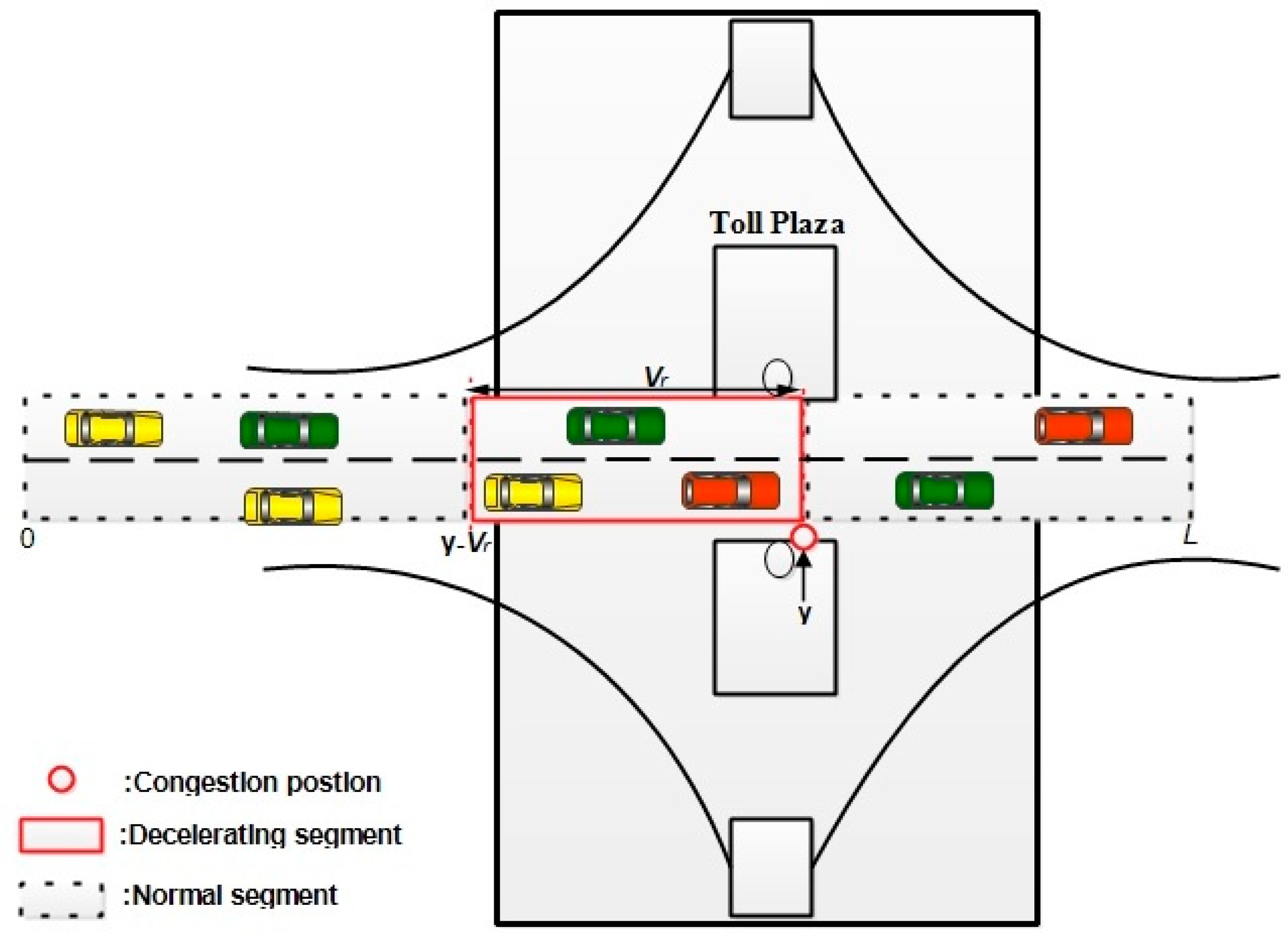
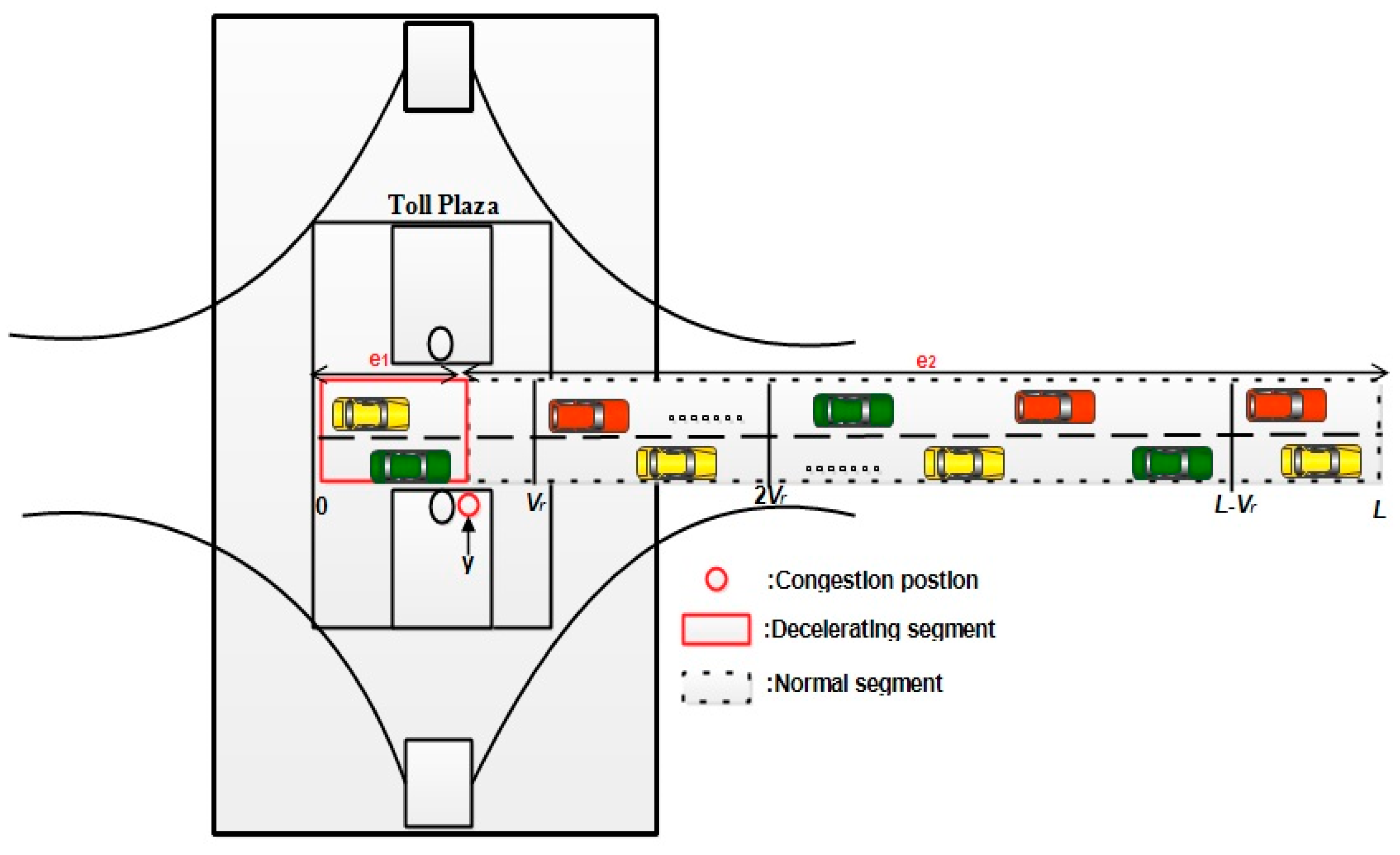
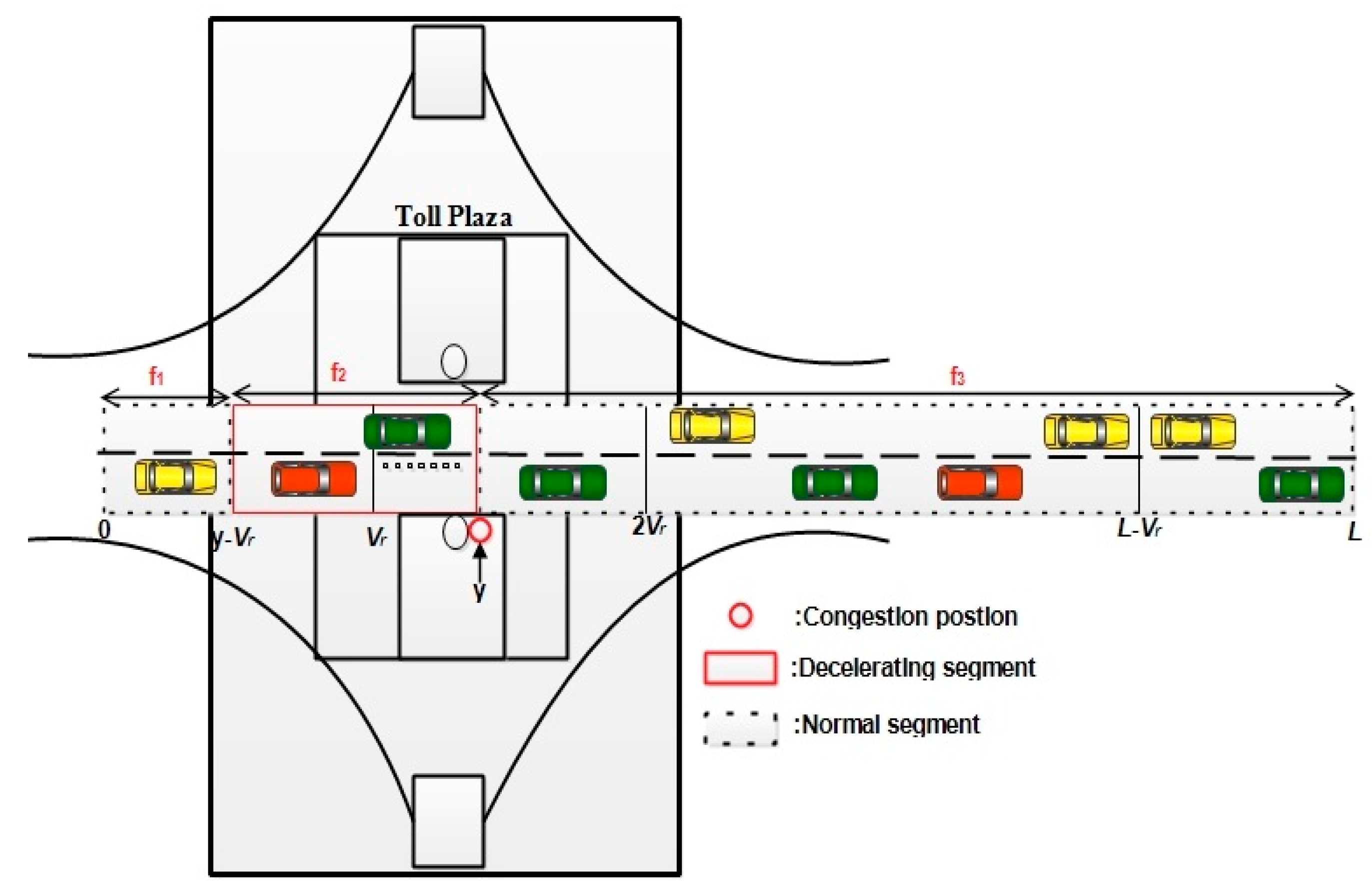
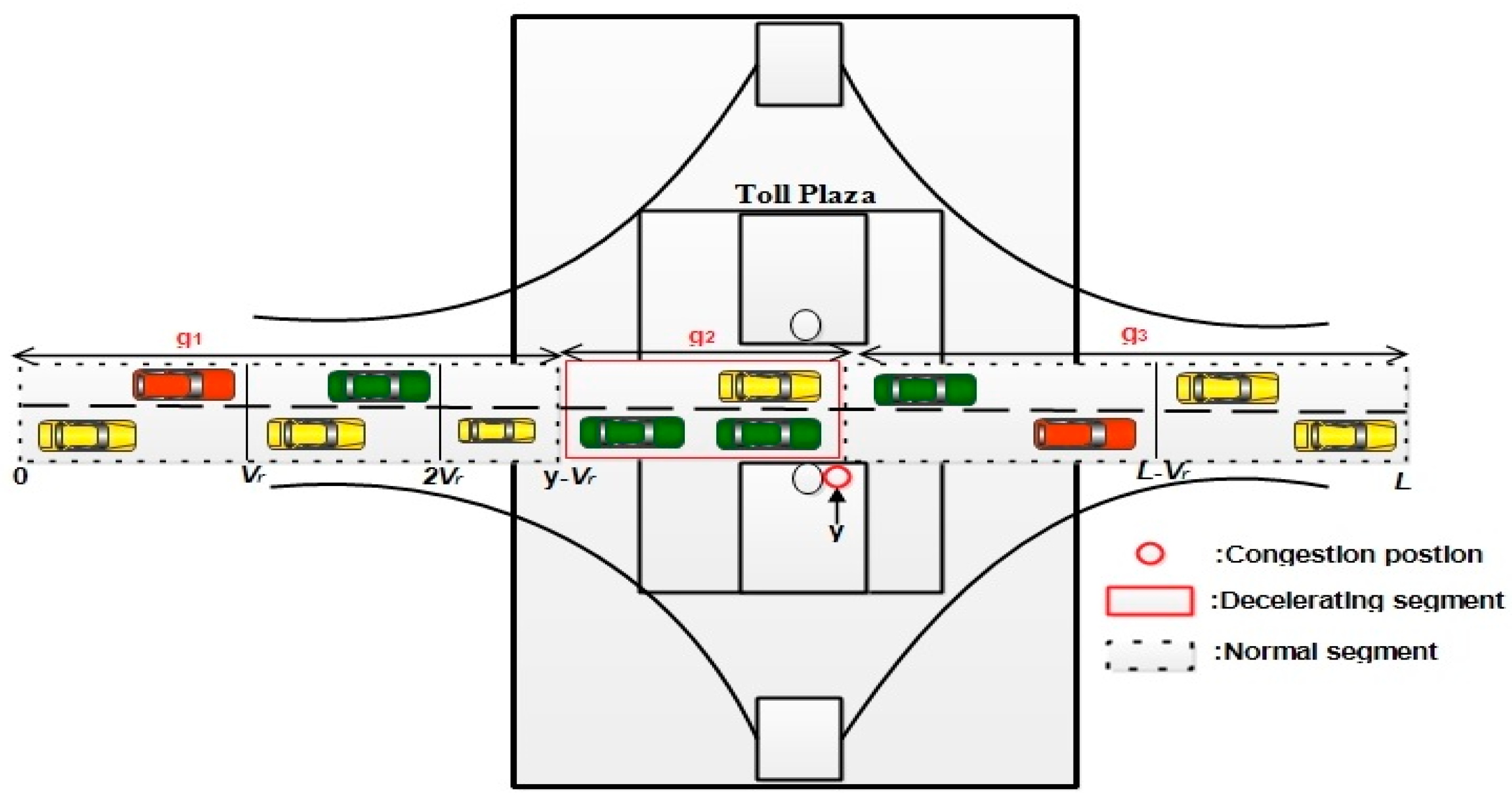
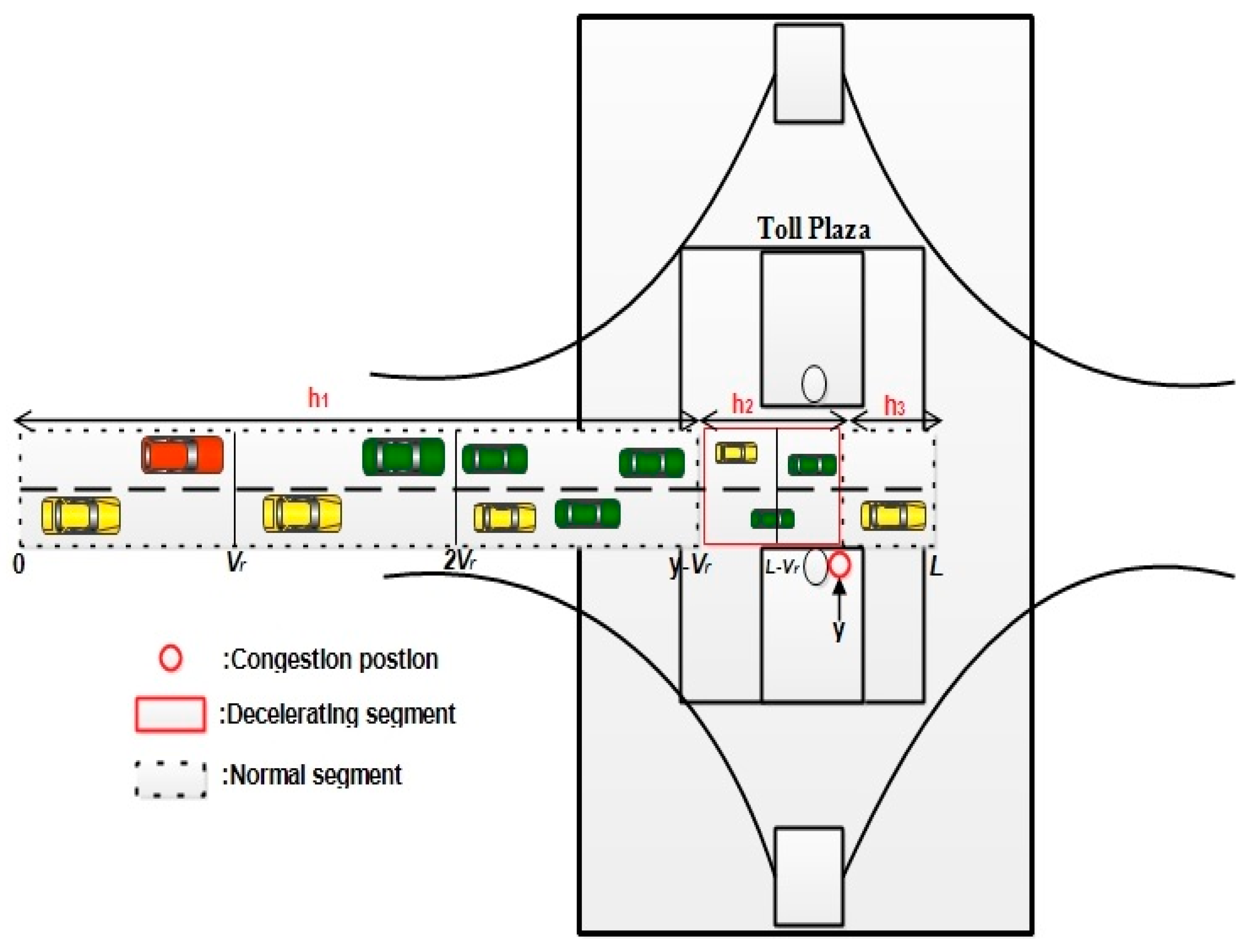
3.1. System Model

The system model is based on a one-way highway road with one toll plaza as depicted in Figure 1. $\left[0,L\right]$ denotes the road, where L is the length of road. The toll plaza is situated at position $y ϵ\left[0,L\right]$, and $y$ is distributed equivalently in $\left[0,L\right]$. As defined earlier, the segment of road could be in a highway scenario, guaranteeing that the congestion at the toll plaza could make the vehicles behind within communication range $V_r$ reduce their speed instead of blocking the flow of traffic. Therefore, the toll plaza divides the road with various vehicle speeds into two or three sub-segments. The normal speed $v_1$ is for vehicles traveling along the normal segment. While vehicles traveling in the decelerating segment reduced with safe speed$v_2, (v_1\ge v_2)$. The accelerating and decelerating factors of vehicles at other complicated points of the two different segments are neglected in this paper. For example, usually, the velocity of standard vehicles is faster than 5.9 $\mathrm{m}/{\mathrm{s}}^2$, which shows the transition of speed within a distance of 10 $\mathrm{m}/\mathrm{s}$ can be obtained in 1.6 s. The time of transition is shorter than the time that the vehicles stay within that segment of road. The Poisson process is followed by the arriving vehicles at road entrance with arrival rate$\mathsf{\lambda }$. Therefore, in normal segments [$0, y-V_r$] and $\left[y,L\right]$, the Poisson distribution is followed by the number of vehicles per meter with $p_1=\mathsf{\lambda }/v_1$, where $p_2=\mathsf{\lambda }/v_2$ in the decelerating segment [$y-V_r,y$].

Figure 1. Considered scenario.

The vehicles’ connectivity when traveling on the highway is defined as follows:

(1)

Two vehicles are connected if the distance between them does not exceed the transmission range of a vehicle.

(2)

If any two vehicles on the sub-segment are connected, the sub-segment will be connected.

(3)

The two sub-segments connect if there are at least two vehicles that are connected on these two sub-segments.

(4)

The road is connected if at least two adjacent road segments are connected.

3.2. Connectivity Probability

Suppose the location of the toll plaza on the road is distributed uniformly $y ϵ\left[0,L\right]$. The connectivity can be analyzed under four cases (followed by the assumption $>3V_r$):

(1)

D1: The location of the toll plaza is $y ϵ\left[0,V_r\right].$

(2)

D2: The location of the toll plaza is $y ϵ\left[V_r,2V_r\right].$

(3)

D3: The location of the toll plaza is $y ϵ\left[2V_r,L-V_r\right].$

(4)

D4: The location of the toll plaza is $y ϵ\left[L-V_r,L\right].$

In D1, if the vehicles are traveling on segment [$0, y$], the road segment is connected. Therefore, it is only important to analyze the connectivity of road segments [$0, y$] and$\left[y,L\right]$. If the vehicles are not available on segment $\left[0,y\right],$ then the connectivity of segment$\left[y,L\right]$should be analyzed. To better understand the concept, road $\left[0,L\right]$ is divided into two sub-segments: [$0, y$] and $[y,L$], which are denoted by $e_1$, and $e_2$, respectively, as shown in Figure 2.

Figure 2. Demonstration of D1$:yϵ\left[0,V_r\right]$.

To better understand the analysis, the main notations are defined in Table 1.

Table 1. Notations.

Symbol	Meaning
$P_r\left\{X\right\}$	represents the probability of occurring event X.
$H_s$	represents the vehicle's availability on s segment of road.
$D_s$	represents the event that s segment of road is connected.
$\overline{H_s}$	represents the unavailability of vehicles on s segment of road.
$\overline{D_s}$	represents the s segment is not connected.
Suppose $D_{s1,s2}$ represents the event that segments $s_1$and $s_2$ are connected, i.e., the two vehicles are connected that are traveling on segments $s_1$and$s_2$.

Based on the mathematical properties of the Poisson distribution, the probability that the vehicles are traveling on $e_1$ is specified as

$${\mathrm{P}}_{\mathrm{r}}\left\{H_{e1}\right\}=1- \frac{{(p_2 . y)}^0}{0!}.e^{-p_2 . y}=1-e^{-p_2 . y}$$

(1)

and the probability no vehicles are traveling on segment $e_1$ is specified as

$${\mathrm{P}}_{\mathrm{r}}\left\{\overline{H_{e1}}\right\}=1-{\mathrm{P}}_{\mathrm{r}}\left\{H_{e1}\right\}=e^{-p_2 .y}.$$

(2)

Likewise, the probabilities of the vehicles traveling on $e_2$ and the probabilities of no vehicles traveling on $e_2$ are specified as

$${\mathrm{P}}_{\mathrm{r}}\left\{H_{e2}\right\}=1-e^{-p_1 .\left( L-y\right)}$$

(3)

and

$${\mathrm{P}}_{\mathrm{r}}\left\{\overline{H_{e2}}\right\}=e^{-p_1.\left(L-y\right) },$$

(4)

respectively.

We further performed the analysis by dividing D1 into two sub-cases:

(1)

D1.1: vehicles are traveling on segment$e_1$;

(2)

D1.2: vehicles are not traveling on segment$e_1$.

In D1.1, the vehicles are connected on$e_1$, i.e.,

$${\mathrm{P}}_{\mathrm{r}}\left\{D_{e1}\right\}=1.$$

(5)

Hence, the vehicle’s availability on segment$e_2$ seriously influences network probability. Therefore, the following two sub-cases were considered:

(1)

D1.1.1: vehicles are traveling on$e_2$;

(2)

D1.1.2: vehicles are not traveling on$e_2$.

In D1.1.1, the connectivity probability is analyzed as${\mathrm{P}}_{\mathrm{r}}\left\{D_{e2}\right\}$for the segment$e_2$ and ${\mathrm{P}}_{\mathrm{r}}\left\{D_{e1,e2}\right\}$among segments$e_{1 }$and$e_2$.

As defined by Author et al. [24], the connectivity probability of one road segment using the Poisson process is defined as

$${\mathrm{P}}_{\mathrm{r}}\left\{{\mathsf{\lambda }}_p, V_r,s\right\}=e^{-{\mathsf{\lambda }}_p.s}{\displaystyle \sum }_{j=0}^{⎣s/V_r⎦}\frac{{(-1)}^j}{j^{!}} {[{\mathsf{\lambda }}_p\left(s-j{V}_r\right)]}^{j-1}\times \left[j+{\mathsf{\lambda }}_p\left(s-j{V}_r\right)\right]e^{{\mathsf{\lambda }}_p.\left(s-j{V}_r\right)}$$

(6)

where $s$ is the length of road, the transmission radius of a vehicle is$V_r$, the density of vehicles is ${\mathsf{\lambda }}_p$, and $⎣x⎦$ is the larger integer that is not larger than$x$. Therefore, we obtain

$${\mathrm{P}}_{\mathrm{r}}\left\{D_{e2}\right\}={\mathrm{P}}_{\mathrm{r}}\left\{p_1,V_r,L-y\right\}.$$

(7)

For ${\mathrm{P}}_{\mathrm{r}}\left\{D_{e1,e2}\right\}$, the probability of connectivity that two vehicles are connected is first calculated for those are traveling on $e_1$ and$e_2$, respectively. Suppose that vehicle $V_1$ is positioned at $l{V}_1$ $\left(0\le l{V}_1\le y\right)$ on $e_1$ and vehicle $V_2$ is positioned at $l{V}_2$ $\left(y\le l{V}_2\le L\right)$ on $e_2$. $l{V}_1$ and $l{V}_2$ are distributed uniformly on $e_{1 }$and $e_2$, respectively Therefore, the probability density functions of $l{V}_1$ and $l{V}_2$ are defined respectively as

$$fl{V}_1\left(w\right)=\frac{1}{y},0\le w\le y$$

(8)

and

$$fl{V}_2\left(x\right)=\frac{1}{L-y},y\le x\le L.$$

(9)

Let $P{V}_1{V}_2$ represent the vehicle’s probability that $V_1$ and $V_2$ are directly associated, i.e., the probability that the space between vehicle $V_1$ and $V_2$ is not larger than the communication radius $V_r$. Therefore:

$$fl{V}_2\left(x\right)=\frac{1}{L-y},y\le x\le L$$

(10)

Subsequently, a probability analysis of the two vehicles that are positioned at $e_1,e_2$ and are connected to each other was conducted. Based on $P{V}_1{V}_2,$ the probability that a vehicle positioned at $e_2$ cannot communicate directly with any of the vehicles at $e_1$ is defined as

$$q_{e_1,e_2}=\frac{1}{1-{\mathrm{P}}_{\mathrm{r}}\left\{\overline{H_{e1}}\right\}} {\displaystyle \sum }_{k=1}^{\infty }{(1-P{V}_1{V}_2)}^k{\mathrm{P}}_{\mathrm{r}}\left\{n_{e1}=k\right\}=\frac{1}{e^{p2y}-1}(e^{\frac{\left(2L-2V_r-y\right)}{2\left(L-y\right).p_{2^y}}}-1)$$

(11)

where ${\mathrm{P}}_{\mathrm{r}}\left\{n_s=k\right\}$ is the probability that there are $k$ vehicles traveling on segment $s$. Therefore, the probability that $e_1,e_2$ are connected is defined as

$${\mathrm{P}}_{\mathrm{r}}\left\{D_{e_1,e_2}\right\}=1-{\displaystyle \sum }_{k=0}^{\infty }{q}_{e_1,e_2}{}^k.{\mathrm{P}}_{\mathrm{r}}\{n_{e2}=k\}=1-e^{-p1\left(L-y\right)\left(1-q_{e_1,e_2}\right).}$$

(12)

Based on Equations (5), (7), and (12), the probability of connectivity of the road $\left[0,L\right]$ in D 1.1.1 is defined as

$$p_{111}={\mathrm{P}}_{\mathrm{r}}\left\{D_{e_1}\right\}.{\mathrm{P}}_{\mathrm{r}}\left\{D_{e_2}\right\}.{\mathrm{P}}_{\mathrm{r}}\left\{D_{e_1,e_2}\right\}.$$

(13)

In D 1.1.2, as there are no vehicles traveling on segment $e_2$, the probability of the connected road $\left[0,L\right]$in D 1.1.2 is defined as

$$p_{112}={\mathrm{P}}_{\mathrm{r}}\left\{D_{e1}\right\}=1.$$

(14)

According to the above two sub-cases in D1.1, the road’s $\left[0,L\right]$ connectivity probability is defined as:

$$p_{11}={\mathrm{P}}_{\mathrm{r}}\left\{H_{e2}\right\}.p_{111}+{\mathrm{P}}_{\mathrm{r}}\left\{\overline{H_{e2}}\right\}.p_{112}.$$

(15)

In D1.2, the connectivity probability only needs to be calculated for segment $\left[y,L\right]$, i.e.,

$$p_{12}={\mathrm{P}}_{\mathrm{r}}\left\{D_{e2}\right\}.$$

(16)

Based on the analysis above, the road $\left[0,L\right]$ connectivity probability in D1, is defined as:

$$p_1={\mathrm{P}}_{\mathrm{r}}\left\{H_{e1}\right\}.p_{11}+{\mathrm{P}}_{\mathrm{r}}\left\{\overline{H_{e1}}\right\}.p_{12}.$$

(17)

In D2, the road $\left[0,L\right]$ is separated into three sub-segments: $\left[0,y-V_r\right], \left[y-V_r,y\right],$ and $\left[y,L\right]$, which are represented by $f_1,f_2,$ and$f_3$, respectively, as depicted in Figure 3.

Figure 3. Demonstration of D2$: y ϵ \left[V_r,2V_r\right]$.

The probabilities listed below can be easily obtained following the procedure used for D1:

$${\mathrm{P}}_{\mathrm{r}}\left\{H_{f1 }\right\}=1-e^{-p_1\left(y-V_r\right)}$$

(18)

$${\mathrm{P}}_{\mathrm{r}}\left\{H_{f2 }\right\}=1-e^{-p_2{V}_r}$$

(19)

$${\mathrm{P}}_{\mathrm{r}}\left\{H_{f3 }\right\}=1-e^{-p_1\left(L-y\right)}$$

(20)

$${\mathrm{P}}_{\mathrm{r}}\left\{\overline{H_{f1}}\right\}=e^{-p_1 \left(y-V_r\right)}$$

(21)

$${\mathrm{P}}_{\mathrm{r}}\left\{\overline{H_{f2}}\right\}=e^{-p_2{V}_r}$$

(22)

$${\mathrm{P}}_{\mathrm{r}}\left\{\overline{H_{f3}}\right\}=e^{-p_1\left(y-V_r\right)}$$

(23)

If the vehicles are traveling on segment$f_2,$ D2 can be divided two sub-cases:

(1)

D2.1: vehicles are traveling on$f_{2 }$;

(2)

D2.2: vehicles are not traveling on$f_2$.

In D2.1, vehicles are connected on $f_2$, i.e.,

$${\mathrm{P}}_{\mathrm{r}}\left\{D_{f2}\right\}=1.$$

(24)

We considered the four following sub-cases:

(1)

D2.1.1: vehicles are traveling on $f_{1 }$and $f_{3 }$;

(2)

D2.1.2: vehicles are traveling on$f_1$, but vehicles are not traveling on $f_{3 }$;

(3)

D2.1.3: vehicles are not traveling on $f_1$, but vehicles are traveling on $f_{3 };$

(4)

D2.1.4: vehicles are not traveling on either segment $f_{1 }$or $f_3$.

In D2.1.1, the vehicles are connected on$f_1$, i.e.,

$${\mathrm{P}}_{\mathrm{r}}\left\{D_{f1}\right\}=1.$$

(25)

Therefore, it is only important to analyze the connectivity probabilities ${\mathrm{P}}_{\mathrm{r}}\left\{D_{f3}\right\}$, ${\mathrm{P}}_{\mathrm{r}}\left\{D_{f1,f2}\right\}$, and ${\mathrm{P}}_{\mathrm{r}}\left\{D_{f2,f3}\right\}.$

For the connectivity probability, ${\mathrm{P}}_{\mathrm{r}}\left\{D_{f3}\right\}$ could be defined as

$${\mathrm{P}}_{\mathrm{r}}\left\{D_{f3}\right\}={\mathrm{P}}_{\mathrm{r}}\left\{ p_1,V_r,L-y\right\}.$$

(26)

By applying the same method as with${\mathrm{P}}_{\mathrm{r}}\left\{D_{e1,e2}\right\}$, the probability${\mathrm{P}}_{\mathrm{r}}\left\{D_{f1,f2}\right\}$ that both of the segments $f_{1 }$and $f_{2 }$are connected is defined as

$${\mathrm{P}}_{\mathrm{r}}\left\{D_{f1,f2}\right\}=1-e^{-p2V_r\left(1-q_{f_1,f_2}\right)}$$

(27)

where

$$q_{f_1,f_2}=\frac{1}{e^{p1\left(y-V_r\right)}-1}\left(e^{{(y-V_r)}^2/2V_r.p1}-1\right).$$

(28)

Likewise, the probability ${\mathrm{P}}_{\mathrm{r}}\left\{D_{f2,f3}\right\}$ both segments $f_{2 }$ and $f_{3 }$ are connected is defined as

$${\mathrm{P}}_{\mathrm{r}}\left\{D_{f2,f3}\right\}=1-e^{-p1\left(L-y\right)\left(1-q_{f_2,f_3}\right)}$$

(29)

where

$$q_{f_2,f_3}=\frac{1}{e^{p2V_r}-1}\left(e^{(1-V_r/2\left(L-y\right)).p_2{V}_r}-1\right).$$

(30)

Hence, the probability of the connectivity of the road $\left[0,L\right]$ in D 2.1.1 is defined as

$$p_{211}={\mathrm{P}}_{\mathrm{r}}\left\{D_{f1}\right\}.{\mathrm{P}}_{\mathrm{r}}\left\{D_{f2}\right\}.{\mathrm{P}}_{\mathrm{r}}\left\{D_{f3}\right\}.{\mathrm{P}}_{\mathrm{r}}\left\{D_{f1,f2}\right\}.{\mathrm{P}}_{\mathrm{r}}\left\{D_{f2,f3}\right\}.$$

(31)

In D2.1.2, the vehicles are not traveling on segment $f_3$. Hence, the probability of connectivity of the road $\left[0,L\right]$ is defined as

$$p_{212}={\mathrm{P}}_{\mathrm{r}}\left\{D_{f1}\right\}.{\mathrm{P}}_{\mathrm{r}}\left\{D_{f2}\right\}.{\mathrm{P}}_{\mathrm{r}}\left\{D_{f1,f2}\right\}.$$

(32)

In D2.1.3, the vehicles are not traveling on segment $f_1$. Hence, the probability of connectivity of the road $\left[0,L\right]$ is defined as

$$p_{213}={\mathrm{P}}_{\mathrm{r}}\left\{D_{f2}\right\}.{\mathrm{P}}_{\mathrm{r}}\left\{D_{f3}\right\}.{\mathrm{P}}_{\mathrm{r}}\left\{D_{f2,f3}\right\}.$$

(33)

In D2.1.4, the vehicles are not traveling on segments $f_1$ or $f_3$. Hence, the probability of connectivity of the road $\left[0,L\right]$ is defined as

$$p_{214}={\mathrm{P}}_{\mathrm{r}}\left\{D_{f2}\right\}=1.$$

(34)

For the above four sub-cases, the probability of connectivity in D2.1 is defined as:

$$\begin{array}{c}{p}_{21}={\mathrm{P}}_{\mathrm{r}}\left\{H_{f1}\right\}.{\mathrm{P}}_{\mathrm{r}}\left\{H_{f3}\right\}.p_{211}+{\mathrm{P}}_{\mathrm{r}}\left\{H_{f1}\right\}.{\mathrm{P}}_{\mathrm{r}}\left\{\overline{H_{f3}}\right\}.p_{212}+{\mathrm{P}}_{\mathrm{r}}\left\{\overline{H_{f1}}\right\}.{\mathrm{P}}_{\mathrm{r}}\left\{H_{f3}\right\}.p_{213}+\\ {\mathrm{P}}_{\mathrm{r}}\left\{\overline{H_{f1}}\right\}.{\mathrm{P}}_{\mathrm{r}}\left\{\overline{H_{f3}}\right\}.p_{214}.\end{array}$$

(35)

In D2.2, there are no vehicles traveling on $f_2$. There is a possibility that the road $\left[0,L\right]$ is connected if any one of the two below sub-cases occurs:

(1)

D2.2.1: vehicles are traveling on $f_1$ but vehicles are not traveling on $f_{3 }$;

(2)

D2.2.2: vehicles are not traveling on $f_1$ but vehicles are traveling on $f_{3 }$.

In D2.2.1, the probability of connectivity of the road $\left[0,L\right]$ is defined as

$$p_{221}={\mathrm{P}}_{\mathrm{r}}\left\{D_{f1}\right\}=1.$$

(36)

Hence in D2.2.2, the probability of connectivity of the road $\left[0,L\right]$ is defined as

$$p_{222}={\mathrm{P}}_{\mathrm{r}}\left\{D_{f3}\right\}=1.$$

(37)

Concerning the above two sub-cases, the probability of connectivity in D2.2 is defined as:

$$p_{22}={\mathrm{P}}_{\mathrm{r}}\left\{H_{f1}\right\}.{\mathrm{P}}_{\mathrm{r}}\left\{\overline{H_{f3}}\right\}.p_{211}+{\mathrm{P}}_{\mathrm{r}}\left\{\overline{H_{f1}}\right\}.{\mathrm{P}}_{\mathrm{r}}\left\{H_{f3}\right\}.p_{222}.$$

(38)

Given the analysis mentioned above for D2, the probability of connectivity of the road $\left[0,L\right]$ in D2 is defined as

$$p_2={\mathrm{P}}_{\mathrm{r}}\left\{H_{f2}\right\}.p_{21}+{\mathrm{P}}_{\mathrm{r}}\left\{\overline{H_{f2}}\right\}.p_{22}.$$

(39)

In D3, the road $\left[0,L\right]$ is separated into three sub-segments: $\left[0,y-V_r\right], \left[y-V_r,y\right],$ and $\left[y,L\right]$, which are represented by $g_1,g_2,$ and $g_3$, respectively, as depicted in Figure 4.

Figure 4. Demonstration of D3$: y ϵ \left[2V_r,L-V_r\right]$.

The probabilities given below are obtained:

$${\mathrm{P}}_{\mathrm{r}}\left\{H_{g1 }\right\}=1-e^{-p_1\left(y-V_r\right)}$$

(40)

$${\mathrm{P}}_{\mathrm{r}}\left\{H_{g2 }\right\}=1-e^{-p_2{V}_r}$$

(41)

$${\mathrm{P}}_{\mathrm{r}}\left\{H_{g3 }\right\}=1-e^{-p_1\left(L-y\right)}$$

(42)

$${\mathrm{P}}_{\mathrm{r}}\left\{\overline{H_{g1}}\right\}=e^{-p_1 \left(y-V_r\right)}$$

(43)

$${\mathrm{P}}_{\mathrm{r}}\left\{\overline{H_{g2}}\right\}=e^{-p_2{V}_r}$$

(44)

$${\mathrm{P}}_{\mathrm{r}}\left\{\overline{H_{g3}}\right\}=e^{-p_1\left(L-y\right)}$$

(45)

If the vehicles are traveling on segment $g_2,$ D3 can be divided into the following two sub-cases:

(1)

D3.1: vehicles are traveling on $g_{2 }$;

(2)

D3.2: vehicles are not traveling on$g_2$.

In D3.1, vehicles are connected on $g_2$, i.e.,

$${\mathrm{P}}_{\mathrm{r}}\left\{D_{g2}\right\}=1.$$

(46)

We considered the following four sub-cases:

(1)

D3.1.1: vehicles are traveling on $g_{1 }$and $g_3$;

(2)

D3.1.2: vehicles are traveling on $g_1$ but not on $g_3$;

(3)

D3.1.3: vehicles are not traveling on $g_1$ but are on $g_3$;

(4)

D3.1.4: vehicles are not traveling on either segment $g_{1 }$or $g_3$.

In D3.1.1, the connectivity probabilities of ${\mathrm{P}}_{\mathrm{r}}\left\{D_{g1}\right\}$, ${\mathrm{P}}_{\mathrm{r}}\left\{D_{g3}\right\},{\mathrm{P}}_{\mathrm{r}}\left\{D_{g2,g1}\right\}$, and ${\mathrm{P}}_{\mathrm{r}}\left\{D_{g2,g3}\right\}$ must be analyzed. Probabilities ${\mathrm{P}}_{\mathrm{r}}\left\{D_{g1}\right\}$ and ${\mathrm{P}}_{\mathrm{r}}\left\{D_{g3}\right\}$ can be defined as

$${\mathrm{P}}_{\mathrm{r}}\left\{D_{g1}\right\}={\mathrm{P}}_{\mathrm{r}}\left\{p_1,V_r,y-V_r\right\}$$

(47)

and

$${\mathrm{P}}_{\mathrm{r}}\left\{D_{g3}\right\}={\mathrm{P}}_{\mathrm{r}}\left\{p_1,V_r,L-y\right\}$$

(48)

By applying the same method as for ${\mathrm{P}}_{\mathrm{r}}\left\{D_{e1,e2}\right\}$, the probability ${\mathrm{P}}_{\mathrm{r}}\left\{D_{g2,g1}\right\}$ that both segments $g_{2 }$and $g_{1 }$are connected is defined as

$${\mathrm{P}}_{\mathrm{r}}\left\{D_{g2,g1}\right\}=1-e^{-p1\left(y-V_r)(1-q_{g2,g_1}\right)}$$

(49)

where

$$q_{g_2,g_1}=\frac{1}{e^{p2V_r}-1}\left(e^{\left(1-V_r/2\left(y-V_r\right)\right).e^{p2V_r}}-1\right).$$

(50)

Hence, the probability ${\mathrm{P}}_{\mathrm{r}}\left\{D_{g2,g3}\right\}$ that both segments $g_{2 }$ and $g_3$ are connected is defined as

$${\mathrm{P}}_{\mathrm{r}}\left\{D_{g2,g3}\right\}=1-e^{-p1\left(L-y\right)\left(1-q_{g_2,g_3}\right)}$$

(51)

where

$$q_{g_2,g_3}=\frac{1}{e^{p2V_r}-1}\left(e^{(1-V_r/2\left(L-y\right)).p2V_r}-1\right).$$

(52)

Hence, the probability of the connectivity of the road $\left[0,L\right]$ in D 3.1.1 is defined as

$$p_{311}={\mathrm{P}}_{\mathrm{r}}\left\{D_{g1}\right\}.{\mathrm{P}}_{\mathrm{r}}\left\{D_{g2}\right\}.{\mathrm{P}}_{\mathrm{r}}\left\{D_{g3}\right\}.{\mathrm{P}}_{\mathrm{r}}\left\{D_{g2,g1}\right\}.{\mathrm{P}}_{\mathrm{r}}\left\{D_{g2,g3}\right\}.$$

(53)

In D3.1.2, the vehicles are not traveling on segment $g_3$. Hence, the probability of connectivity of the road $\left[0,L\right]$ is defined as

$$p_{312}={\mathrm{P}}_{\mathrm{r}}\left\{D_{g1}\right\}.{\mathrm{P}}_{\mathrm{r}}\left\{D_{g2}\right\}.{\mathrm{P}}_{\mathrm{r}}\left\{D_{g2,g1}\right\}.$$

(54)

In D3.1.3, the vehicles are not traveling on segment $g_1$. Hence, the probability of connectivity of the road $\left[0,L\right]$ is defined as

$$p_{313}={\mathrm{P}}_{\mathrm{r}}\left\{D_{g2}\right\}.{\mathrm{P}}_{\mathrm{r}}\left\{D_{g3}\right\}.{\mathrm{P}}_{\mathrm{r}}\left\{D_{g2,g3}\right\}.$$

(55)

In D3.1.4, the vehicles are not traveling on segments $g_{1 }$ or $g_3$. Hence, the probability of connectivity of the road $\left[0,L\right]$ is defined as

$$p_{314}={\mathrm{P}}_{\mathrm{r}}\left\{D_{g2}\right\}=1.$$

(56)

Given the above four sub-cases, the probability of connectivity in D3.1 is defined as

$$\begin{array}{c}{p}_{31}={\mathrm{P}}_{\mathrm{r}}\left\{H_{g1}\right\}.{\mathrm{P}}_{\mathrm{r}}\left\{H_{g3}\right\}.p_{311}+{\mathrm{P}}_{\mathrm{r}}\left\{H_{g1}\right\}.{\mathrm{P}}_{\mathrm{r}}\left\{\overline{H_{g3}}\right\}.p_{312}+{\mathrm{P}}_{\mathrm{r}}\left\{\overline{H_{g1}}\right\}.{\mathrm{P}}_{\mathrm{r}}\left\{H_{g3}\right\}.p_{313}+\\ {\mathrm{P}}_{\mathrm{r}}\left\{\overline{H_{g1}}\right\}.{\mathrm{P}}_{\mathrm{r}}\left\{\overline{H_{g3}}\right\}.p_{314}.\end{array}$$

(57)

In D3.2, there are no vehicles traveling on ${\mathrm{g}}_2$. There is the possibility that the road $\left[0,\mathrm{L}\right]$ is connected if either of the subcases given below occurs:

(1)

D3.2.1: vehicles are traveling on $g_1$ but not on $g_3$

(2)

D3.2.2: vehicles are not traveling on $g_1$ but are on $g_{3 }$

In D3.2.1, the probability of the connectivity of the road $\left[0,L\right]$ is defined as

$$p_{321}={\mathrm{P}}_{\mathrm{r}}\left\{D_{g1}\right\}.$$

(58)

In D3.2.2, the probability of connectivity of the road $\left[0,L\right]$ is defined as

$$p_{322}={\mathrm{P}}_{\mathrm{r}}\left\{D_{g3}\right\}.$$

(59)

Given the above two sub-cases, the probability of connectivity in D3.2 is defined as

$$p_{32}={\mathrm{P}}_{\mathrm{r}}\left\{H_{g1}\right\}.{\mathrm{P}}_{\mathrm{r}}\left\{\overline{H_{g3}}\right\}.p_{321}+{\mathrm{P}}_{\mathrm{r}}\left\{\overline{H_{g1}}\right\}.{\mathrm{P}}_{\mathrm{r}}\left\{H_{g3}\right\}.p_{322}.$$

(60)

Given the above analysis, for D3, the probability of connectivity of the road $\left[0,L\right]$ is defined as

$$p_3={\mathrm{P}}_{\mathrm{r}}\left\{H_{g2}\right\}.p_{31}+{\mathrm{P}}_{\mathrm{r}}\left\{\overline{H_{g2}}\right\}.p_{32}.$$

(61)

In D4, the road $\left[0,L\right]$ is separated into three sub-segments: $\left[0,y-V_r\right], \left[y-V_r,y\right],$ and $\left[y,L\right]$, which are represented by $h_1,h_2,$ and $h_3$, respectively, as depicted in Figure 5.

Figure 5. Demonstration of D4$: y ϵ \left[L-V_r,L\right]$.

The probabilities listed below are obtained:

$${\mathrm{P}}_{\mathrm{r}}\left\{H_{h1 }\right\}=1-e^{-p_1\left(y-V_r\right)}$$

(62)

$${\mathrm{P}}_{\mathrm{r}}\left\{H_{h2 }\right\}=1-e^{-p_2{V}_r}$$

(63)

$${\mathrm{P}}_{\mathrm{r}}\left\{H_{h3 }\right\}=1-e^{-p_1\left(L-y\right)}$$

(64)

$${\mathrm{P}}_{\mathrm{r}}\left\{\overline{H_{h1}}\right\}=e^{-p_1 \left(y-V_r\right)}$$

(65)

$${\mathrm{P}}_{\mathrm{r}}\left\{\overline{H_{h2}}\right\}=e^{-p_2{V}_r}$$

(66)

$${\mathrm{P}}_{\mathrm{r}}\left\{\overline{H_{h3}}\right\}=e^{-p_1\left(L-y\right)}$$

(67)

If the vehicles are traveling on segment $h_2,$ D4 can be separated into two sub-cases:

(1)

D4.1: vehicles are traveling on $h_{2 }$;

(2)

D4.2: vehicles are not traveling on $h_2$.

In D4.1, the vehicles are connected on $h_2$, i.e.,

$${\mathrm{P}}_{\mathrm{r}}\left\{D_{h2}\right\}=1.$$

(68)

We considered the following four sub-cases:

(1)

D4.1.1: vehicles are traveling on $h_{1 }$and $h_3$;

(2)

D4.1.2: vehicles are traveling on $h_1$ but not on $h_3$;

(3)

D4.1.3: vehicles are not traveling on $h_1$ but are on $h_3$;

(4)

D4.1.4: vehicles are not traveling on $h_{1 }$or $h_3$.

In D4.1.1, vehicles traveling on $h_3$ are connected, i.e.,

$${\mathrm{P}}_{\mathrm{r}}\left\{D_{h3}\right\}=1.$$

(69)

Hence, the connectivity probabilities of ${\mathrm{P}}_{\mathrm{r}}\left\{D_{h1}\right\}$,${\mathrm{P}}_{\mathrm{r}}\left\{D_{h2,h1}\right\}$, and ${\mathrm{P}}_{\mathrm{r}}\left\{D_{h3,h2}\right\}$ must be analyzed. The probability${\mathrm{P}}_{\mathrm{r}}\left\{D_{h1}\right\}$ is defined as

$${\mathrm{P}}_{\mathrm{r}}\left\{D_{h1}\right\}={\mathrm{P}}_{\mathrm{r}}\left\{p_1,V_r,y-V_r\right\}.$$

(70)

By applying the same method as with ${\mathrm{P}}_{\mathrm{r}}\left\{D_{e1,e2}\right\}$, the probability ${\mathrm{P}}_{\mathrm{r}}\left\{D_{h2,h1}\right\}$ that both segments $h_2$ and $h_{1 }$are connected is defined as

$${\mathrm{P}}_{\mathrm{r}}\left\{D_{h2,h1}\right\}=1-e^{-p1\left(y-V_r)(1-q_{h2,h_1}\right)}$$

(71)

where

$$q_{h_2,h_1}=\frac{1}{e^{p2V_r}-1}\left(e^{\left(1-V_r/2\left(y-V_r\right)\right).e^{p2V_r}}-1\right).$$

(72)

The probability ${\mathrm{P}}_{\mathrm{r}}\left\{D_{h3,h2}\right\}$ that both segments $h_{3 }$ and $h_2$ are connected is defined as:

$${\mathrm{P}}_{\mathrm{r}}\left\{D_{h3,h2}\right\}=1-e^{-p2V_r\left(1-q_{h_3,h_2}\right)}$$

(73)

where

$$q_{h_3,h_2}=\frac{1}{e^{p1\left(L-y\right)}-1}\left(e^{{(L-y)}^{2}p1/2V_r}-1\right).$$

(74)

Hence, the probability of connectivity of the road $\left[0,L\right]$ in D4.1.1 is defined as

$$p_{411}={\mathrm{P}}_{\mathrm{r}}\left\{D_{h1}\right\}.{\mathrm{P}}_{\mathrm{r}}\left\{D_{h2}\right\}.{\mathrm{P}}_{\mathrm{r}}\left\{D_{h3}\right\}.{\mathrm{P}}_{\mathrm{r}}\left\{D_{h2,h1}\right\}.{\mathrm{P}}_{\mathrm{r}}\left\{D_{h3,h2}\right\}.$$

(75)

In D4.1.2, vehicles are not traveling on $h_3$. Hence, the probability of connectivity of the road $\left[0,L\right]$ is defined as

$$p_{412}={\mathrm{P}}_{\mathrm{r}}\left\{D_{h1}\right\}.{\mathrm{P}}_{\mathrm{r}}\left\{D_{h2}\right\}.{\mathrm{P}}_{\mathrm{r}}\left\{D_{h2,h1}\right\}.$$

(76)

In D4.1.3, the vehicles are not traveling on segment$h_1$. Hence, the probability of connectivity of the road $\left[0,L\right]$ is defined as

$$p_{413}={\mathrm{P}}_{\mathrm{r}}\left\{D_{h2}\right\}.{\mathrm{P}}_{\mathrm{r}}\left\{D_{h3}\right\}.{\mathrm{P}}_{\mathrm{r}}\left\{D_{h3,h2}\right\}.$$

(77)

In D4.1.4, the vehicles are not traveling on $h_{1 }$ or $h_3$. Hence, the probability of connectivity of the road $\left[0,L\right]$ is defined as

$$p_{414}={\mathrm{P}}_{\mathrm{r}}\left\{D_{h2}\right\}=1.$$

(78)

Given the above four sub-cases, the probability of connectivity in D4.1 is defined as

$$\begin{array}{c}{p}_{41}={\mathrm{P}}_{\mathrm{r}}\left\{H_{h1}\right\}.{\mathrm{P}}_{\mathrm{r}}\left\{H_{h3}\right\}.p_{411}+{\mathrm{P}}_{\mathrm{r}}\left\{H_{h1}\right\}.{\mathrm{P}}_{\mathrm{r}}\left\{\overline{H_{h3}}\right\}.p_{412}+{\mathrm{P}}_{\mathrm{r}}\left\{\overline{H_{h1}}\right\}.{\mathrm{P}}_{\mathrm{r}}\left\{H_{h3}\right\}.p_{413}+\\ {\mathrm{P}}_{\mathrm{r}}\left\{\overline{H_{h1}}\right\}.{\mathrm{P}}_{\mathrm{r}}\left\{\overline{H_{h3}}\right\}.p_{414}.\end{array}$$

(79)

In D4.2, there are no vehicles traveling on $h_2$. There is the possibility of the road $\left[0,L\right]$ being connected if either of the subcases given below occurs:

(1)

D4.2.1: vehicles are traveling on $h_1$ but are not on $h_{3 }$

(2)

D4.2.2: vehicles are not traveling on $h_1$ but are on $h_{3 }$

In D4.2.1, the probability of connectivity of the road $\left[0,L\right]$ is defined as

$$p_{421}={\mathrm{P}}_{\mathrm{r}}\left\{D_{h1}\right\}.$$

(80)

In D4.2.2, the probability of connectivity of the road $\left[0,L\right]$ is defined as

$$p_{422}={\mathrm{P}}_{\mathrm{r}}\left\{D_{h3}\right\}=1.$$

(81)

Given the above two sub-cases, the probability of connectivity in D4.2 is defined as

$$p_{42}={\mathrm{P}}_{\mathrm{r}}\left\{H_{h1}\right\}.{\mathrm{P}}_{\mathrm{r}}\left\{\overline{H_{h3}}\right\}.p_{411}+{\mathrm{P}}_{\mathrm{r}}\left\{\overline{H_{h1}}\right\}.{\mathrm{P}}_{\mathrm{r}}\left\{H_{h3}\right\}.p_{422}.$$

(82)

For the analysis of D4, the probability of connectivity of the road $\left[0,L\right]$ in D4 is defined as

$$p_4={\mathrm{P}}_{\mathrm{r}}\left\{H_{h2}\right\}.p_{41}+{\mathrm{P}}_{\mathrm{r}}\left\{\overline{H_{h2}}\right\}.p_{42}.$$

(83)

Finally, the road’s $\left[0,L\right]$ connectivity probability including all the analyses given above is defined as

$$p=\frac{1}{L}.\left({{\displaystyle \int }}_0^{V_r}{p}_{1}Ly+{{\displaystyle \int }}_{V_r}^{2V_r}{p}_{2}Ly+{{\displaystyle \int }}_{2V_r}^{L-V_r}{p}_{3}Ly+{{\displaystyle \int }}_{L-V_r}^L{p}_{4}Ly\right).$$

(84)

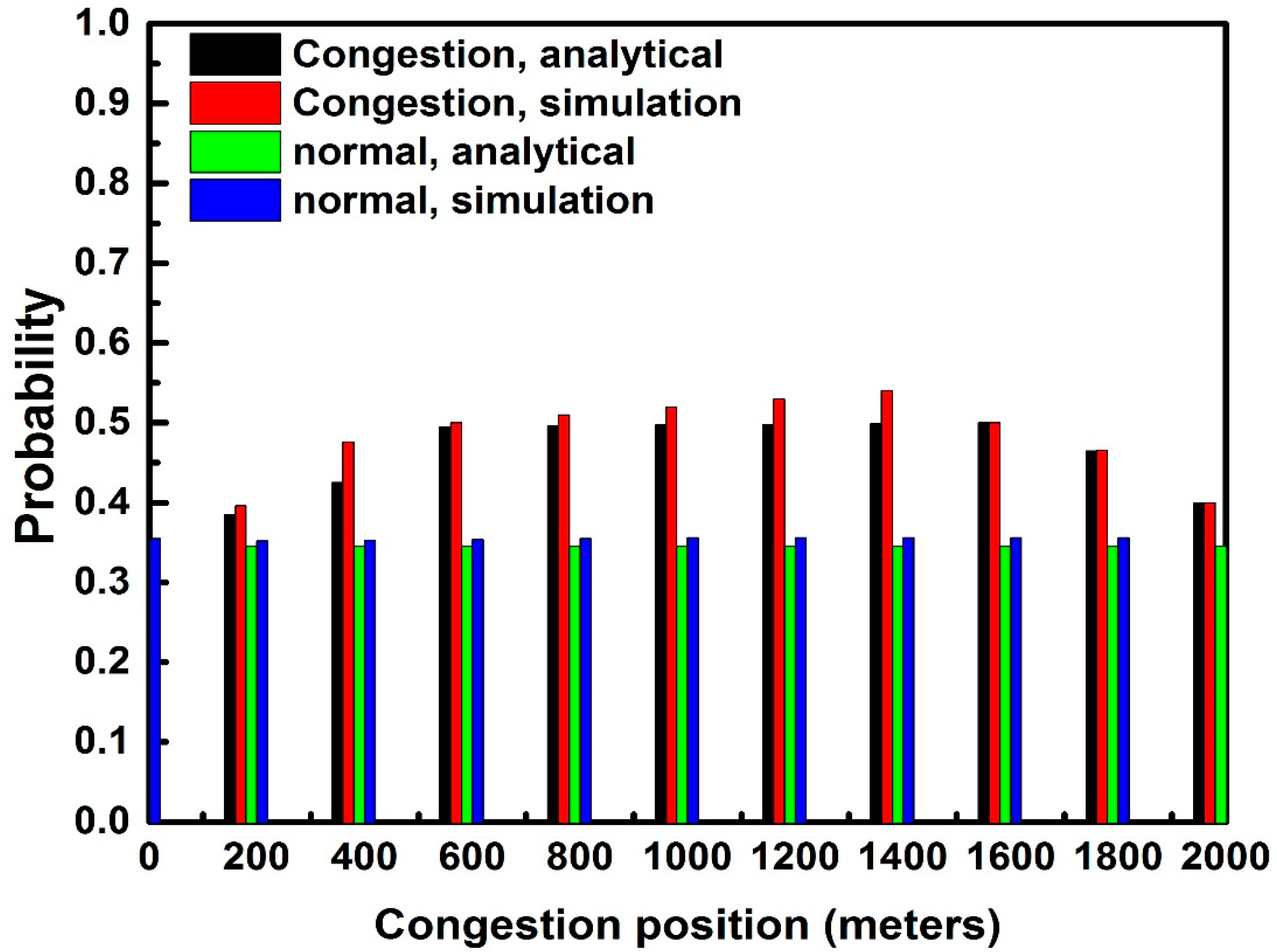
4. Experimental Results and Analysis

4.1. Adaptation of Proposed Model in a Realistic Scenario

With the help of the Poisson process, the connectivity probability of one road segment was defined. In eq 6, the proposed model is not limited to the toll plaza but can be extended to various environments such as smart parking management systems. The performance of the analytical model is based on connectivity probability by considering various parameters that might disturb the highway connectivity, including traveling speed, arrival rate of vehicles, communication range of vehicles, and road length. To prove the applicability of the proposed model in a realistic network environment, we demonstrate the performance of the developed model under various parameters along with increasing and decreasing connectivity probability while maintaining network capacity.

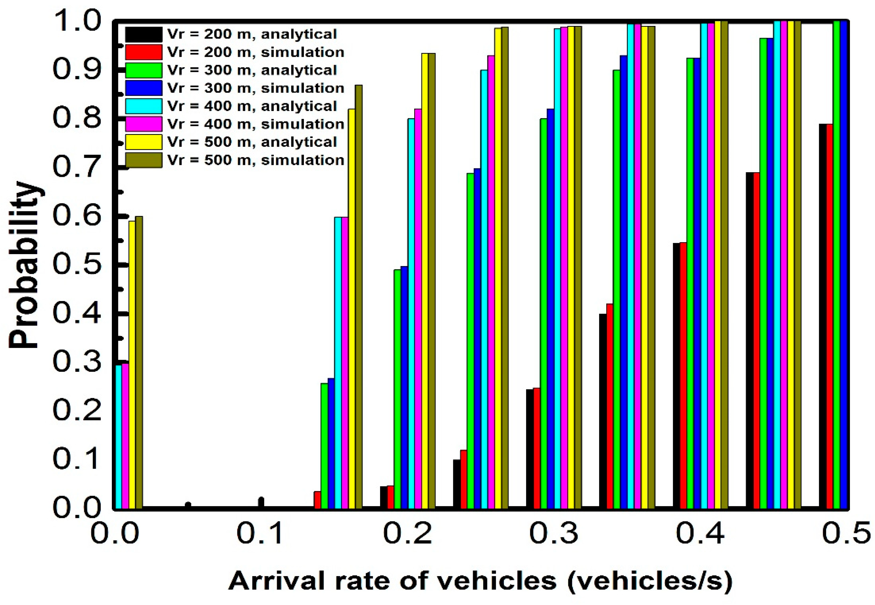
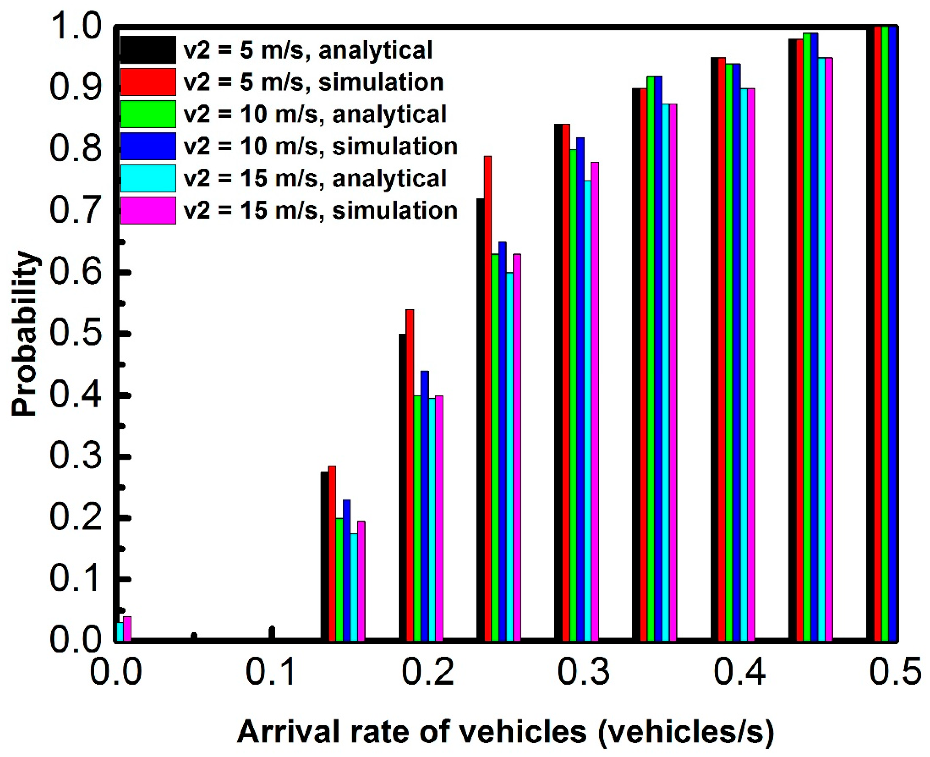
4.2. Impacts of Various Parameters on Connectivity

Our analytical model was verified using simulated results and the impacts of various parameters on the probability of connectivity on the highway, such as arrival rate of vehicles $\mathsf{\lambda },$ the range of communication $V_r$, road length $L$, and normal and safe speed of vehicles $v_1\mathrm{and}{v}_2$, respectively, are highlighted. The results of the analytical model were developed using MATLAB [25] (MathWorks, Natick, MA, USA). A discrete event-driven simulator was used to develop simulation results. In the figures shown below, analytical and simulation results match each other, which confirms the accuracy of the analytical model.

The impact of congestion at the toll plaza on the probability of connectivity is shown in Figure 6. Given congestion at the toll plaza, the probability of connectivity first increases and then decreases at various traffic congestion positions, which means that vehicles on the mid-section of the road severely impact the connectivity.

Figure 6. Effect of congestion position on the probability of connectivity ($Vr$ = 300 m, L = 2000 m, $\lambda$= 0.2 veh/s, $v1$ = 20 m/s, and $v2$ = 10 m/s).

At the point when toll congestion occurs at position 0, the flow of traffic in $\left[0, L\right]$ is similar to the normal situation. Therefore, the probability of connectivity with toll congestion at position 0 is equivalent to that of a normal situation. Of note is that the toll congestion, which caused the vehicles to reduce their speed instead of blocking the flow of traffic, can enhance the connectivity to some extent. Figure 7, Figure 8, Figure 9 and Figure 10 demonstrate the effect of the arrival rate of vehicles on connectivity probability. An increase in connectivity probability is observed with increasing arrival rate of vehicles. As the density of vehicles increases with increasing rate of arrival, the connectivity of the road is also enhanced. Figure 7, Figure 8, Figure 9 and Figure 10 show that the deviation between the analysis and simulation results decreases with increasing arrival rate of vehicles. This is due to large random arrivals and headway distance, which occur with a lower rate of arrival.

Figure 7. Effect of communication range and vehicle arrival rate on connectivity probability (L = 2000 m, $v1$ = 20 m/s, and $v2$ = 10 m/s).

Figure 8. Effect of arrival rate of vehicles and road length on the probability of connectivity ($Vr$ = 300 m and$v1$,$v2$ = 20, 10 m/s, respectively).

Figure 9. Effect of normal speed and arrival rate of vehicles on the probability of connectivity ($v2$ = 10 m/s, L = 2000 m, and $Vr$ = 300 m).

Figure 10. Effect of safe speed and arrival rate of vehicles on the probability of connectivity ($v1$ = 20 m/s, L = 2000 m, and $Vr$ = 300 m).

Figure 7 demonstrates the effect of the communication radius of vehicles on connectivity probability. With increasing communication range of vehicles the probability of connectivity increases, as the two vehicles have a higher chance of being associated with a large range of communication. Of note is that the probability of connectivity increases considerably within the communication range of 200–300 m compared to other gaps in the communication range, which can provide direction for the structure of the transmitting power of the signal.

Figure 8 demonstrates the effect of the whole road length on the probability of connectivity. The probability of connectivity decreases with increasing road length. With consistent probability that two nearby vehicles are associated, a longer road length results in a large number of vehicles, which results in a lower probability of connectivity for all the vehicles. Therefore, the probability of connectivity decreases.

Figure 9 demonstrates the effect of vehicle normal speed on the probability of connectivity. Increasing the normal speed of vehicles results in decreasing connectivity probability, because, in the normal segment, the density of vehicles decreases with increasing normal speed. Also, a larger proportion of the whole road is occupied by the normal segment. The road’s probability of connectivity reduces.

Figure 10 demonstrates the effect of vehicle safe speed on the probability of connectivity. With increasing vehicle safe speed, the connectivity probability slightly decreases, because, in the safe segment, the density of vehicles decreases with increasing safe speed, though a minor section of the whole road is occupied by the decelerating segment. This results in a slight decrease in probability.

5. Conclusions

In this paper, to avoid traffic congestion at a toll plaza, the connectivity of vehicular networks in a one-way highway road scenario was studied. To examine the connectivity probability of the road, a mathematical model was derived. The considered road segment could be a highway, which means that the traffic congestion at a toll plaza could cause the vehicles to reduce their speed instead of blocking the flow of traffic. Nearby vehicles within communication range must be informed when the traffic congestion occurs before reaching the toll plaza so they can reduce their speed to avoid traffic congestion. Once they cross the toll plaza, they can travel at their normal speed. The proposed analytical model considers various parameters that might disturb the connectivity probability, including traveling speed, communication range of vehicles, vehicle arrival rate, and road length. The simulation results confirmed the accuracy of the analytical model, indicating the analytical model is efficient.

In the future, the accelerating and decelerating factors should be considered in a more realistic situation, which would be more complex. It should be noted that we employed the Poisson process for arrival of vehicles; specifically, headway distance follows the exponential distribution. Also, so as to encourage connectivity analysis, the decelerating segment length was fixed to the vehicles’ communication range. Various environments with multiple decelerating segment lengths will be focused on in future.

References

1. Sampigethaya, K.; Li, M.; Huang, L.; Poovendran, R. Amoeba: Robust location privacy scheme for vanet. IEEE J. Sel. Areas Commun. 2007, 25, 1569–1589. [Google Scholar] [CrossRef]
2. Miorandi, D.; Altman, E. Connectivity in One-Dimensional Ad Hoc Networks: A Queueing Theoretical Approach; Springer: New York, NY, USA, 2006. [Google Scholar]
3. Viriyasitavat, W.; Bai, F.; Tonguz, O.K. Dynamics of network connectivity in urban vehicular networks. IEEE J. Sel. Areas Commun. 2011, 29, 515–533. [Google Scholar] [CrossRef]
4. Zhang, W.; Chen, Y.; Yang, Y.; Wang, X.; Zhang, Y.; Hong, X.; Mao, G. Multi-hop transmission probability in infrastructure-based vehicular networks. IEEE J. Sel. Areas Commun. 2012, 30, 740–747. [Google Scholar] [CrossRef]
5. Yousefi, S.; Altman, E.; El-Azouzi, R.; Fathy, M. Improving connectivity in vehicular ad hoc networks: An analytical study. Comput. Commun. 2008, 31, 1653–1659. [Google Scholar] [CrossRef]
6. Cheng, L.; Panichpapiboon, S. Effects of intervehicle spacing distributions on connectivity of vanet: A case study from advanced highway traffic. IEEE Commun. Mag. 2012, 50, 90–97. [Google Scholar] [CrossRef]
7. Keykhaie, S.; Mahmoudifar, A. Study of Connectivity in a Vehicular Ad Hoc Network with Random Node Speed Distribution. In Proceedings of the 2014 6th International Conference on New Technologies, Mobility and Security (NTMS), Dubai, UAE, 30 March–2 April 2014; pp. 1–4. [Google Scholar]
8. Ajeer, V.K.M.; Neelakantan, P.C.; Babu, A.V. Network connectivity of one-dimensional Vehicular Ad hoc Network. In Proceedings of the International Conference on Communications and Signal Processing, Calicut, India, 10–12 February 2011; pp. 241–245. [Google Scholar]
9. Shao, C.; Leng, S.; Fan, B.; Zhang, Y.; Vinel, A.; Jonsson, M. Connectivity-aware Medium Access Control in platoon-based Vehicular Ad Hoc Networks. In Proceedings of the IEEE International Conference on Communications, London, UK, 8–12 June 2015; pp. 3305–3310. [Google Scholar]
10. Yousefi, S.; Altman, E.; El-Azouzi, R.; Fathy, M. Analytical model for connectivity in vehicular ad hoc networks. IEEE Trans. Veh. Technol. 2008, 57, 3341–3356. [Google Scholar] [CrossRef]
11. Wu, J. Connectivity of mobile linear networks with dynamic node population and delay constraint. IEEE J. Sel. Areas Commun. 2009, 27, 1218–1225. [Google Scholar]
12. Zhao, J.; Chen, Y.; Gong, Y. Study of connecting probability based on cluster in vehicular Ad Hoc networks. In Proceedings of the International Conference on Wireless Communications & Signal Processing, Yangzhou, China, 13–15 October 2016; pp. 1–5. [Google Scholar]
13. Khabazian, M.; Ali, M.K.M. A Performance Modeling of Connectivity in Vehicular Ad Hoc Networks. IEEE Trans. Veh. Technol. 2008, 57, 2440–2450. [Google Scholar] [CrossRef]
14. Wang, Y.; Zheng, J. A connectivity analytical model for a highway with an entrance/exit in vehicular ad hoc networks. In Proceedings of the IEEE International Conference on Communications, Kuala Lumpur, Malaysia, 22–27 May 2016; pp. 1–6. [Google Scholar]
15. Panichpapiboon, S.; Pattara-atikom, W. Connectivity requirements forself-organizing traffic information systems. IEEE Trans. Veh. Technol. 2008, 57, 3333–3340. [Google Scholar] [CrossRef]
16. Chen, C.; Du, X.; Pei, Q.; Jin, Y. Connectivity analysis for free-flowtraffic in VANETs: A statistical approach. Int. J. Distrib. Sens. Netw. 2013, 9, 598946. [Google Scholar] [CrossRef]
17. Shao, C.Y.; Leng, S.; Zhang, Y.; Vinel, A.; Jonsson, M. Analysis of connectivity probability in platoon-based vehicular ad hoc networks. In Proceedings of the 2014 International Wireless Communications and Mobile Computing Conference (IWCMC), Nicosia, Cyprus, 4–8 August 2014; pp. 706–711. [Google Scholar]
18. Kong, X.; Xia, F.; Wang, J.; Rahim, A.; Das, S.K. Time-location-relationship combined service recommendation based on taxi trajectory data. IEEE Trans. Ind. Inform. 2017, 13, 1202–1212. [Google Scholar] [CrossRef]
19. Tao, J.; Xu, Y.; Zhang, Z.; Feng, F.; Tong, F.; Dong, F. A resource allocation game with restriction mechanism in VANET cloud. Concur. Comput. Pract. Exp. 2017, 29. [Google Scholar] [CrossRef]
20. Tsiropoulou, E.E.; Baras, J.S.; Papavassiliou, S.; Sinha, S. Rfid-based smart parking management system. Cyber-Phys. Syst. 2017, 3, 22–41. [Google Scholar] [CrossRef]
21. Rose, K.; Eldridge, S.; Chapin, L. The Internet of Things: An Overview—Understanding the Issues and Challenges of a More Connected World; The Internet Society (ISOC): Reston, VA, USA, 2015; p. 80. [Google Scholar]
22. Kong, X.; Li, M.; Ma, K.; Tian, K.; Wang, M.; Ning, Z.; Xia, F. Big Trajectory Data: A Survey of Applications and Services. IEEE Access 2018. [Google Scholar] [CrossRef]
23. Zheng, J.; Wang, Y. Connectivity analysis of vehicles moving on a highway with an entry and exit. IEEE Trans. Veh. Technol. 2018, 67, 4476–4486. [Google Scholar] [CrossRef]
24. Sou, S.I.; Tonguz, O.K. Enhancing VANET connectivity through roadside units on highways. IEEE Trans. Veh. Technol. 2011, 60, 3586–3602. [Google Scholar] [CrossRef]
25. MATLAB. Available online: https://www.mathworks (accessed on 9 February 2019).
Article Metrics
Citations
Article Access Statistics
Multiple requests from the same IP address are counted as one view.