Abstract
In karstic environments, water supply wells are vulnerable to rapid sediment transfer during intense rainfall events, often generating turbidity peaks that disrupt water-treatment operations. In Normandy (France), the high density of sinkholes and the complexity of transport processes in karsts complicate the identification and prioritization of sinkholes requiring mitigation to reduce sediment fluxes at water supply wells. This study aims to quantify the time-lagged impact of each sinkhole on turbidity peaks at a supply well using a cascade modeling approach that couples numerical surface erosion–runoff simulations with deep learning models representing hydrosedimentary responses through the karst network. Surface erosion–runoff was simulated using WaterSed. Hydroclimatic time series and WaterSed model outputs were used as inputs for our deep learning models. Several deep learning architectures were compared and optimized across multiple rounds to identify a best-performing model, which was then interpreted using interpretability methods. Interpretability analyses show that turbidity is primarily controlled by seasonal conditions and short-term rainfall accumulation, while multiple sinkholes contribute jointly to short time lags. Temporal attributions reveal rapid karst response followed by attenuation, consistent with reactive karst behavior. The contribution of each sinkhole to turbidity peaks allows us to identify the most important sinkholes requiring mitigation by stakeholders.
1. Introduction
In karstic landscapes, sediment discharge to karst conduits can occur through rapid and direct transfer via surface erosion processes or through re-suspension of sediments within the karst network itself [1]. During significant rainfall events, this process generates substantial runoff, transporting high sediment loads to both surface streams and karstic conduits.
For water supply, these peaks in sediment load often necessitate additional treatment or, in extreme cases, temporary shutdowns of water-treatment plants [2].
In Normandy (France), the Cretaceous Chalk is intensely karstified, forming broad plateaus with a sparse surface drainage network [3]. Drinking-water supply is drawn predominantly from the karstified Chalk aquifer and, in general, the landscape hosts a high density of sinkholes [3]. Runoff and sediment delivery into sinkholes make drinking-water resources vulnerable following important rainfall episodes. The economic cost linked to the restrictions on the use of drinking water due to excessive sediment load was estimated to be about 5 million euros during the period 1992 to 2018 in Upper Normandy [4].
If a sinkhole has been identified to be connected to a supply well, specific hillslope controls (e.g., upstream grassed buffer strips, hedgerows, and fascines) and/or direct sinkhole works (vegetated ring, flow diversion, and when appropriate sinkhole sealing or engineered filter packs) can be implemented to reduce water turbidity and sanitary risks at the supply well [3].
When several sinkholes have been shown to be connected to a supply well, typically by hydrogeological tracer tests, a catchment-scale modeling approach can be deployed to evaluate and reduce sediment loads. Several approaches exist to model erosion and runoff in karst systems. Empirical hillslope models such as RUSLE [5] are data efficient but they miss spatiotemporal dynamics [6] at the catchment scale. In contrast, physically based models (e.g., WEPP; LISEM) better represent physical processes but require many input parameters and are difficult to scale [7,8].
WaterSed (“Water and Sediment model”) can offer an alternative by focusing on a limited set of parameters, representative of the main processes responsible for soil erosion and runoff. WaterSed is a raster-based distributed model, which simulates runoff and soil erosion for individual rainfall events at spatial scales ranging from agricultural plots to entire watersheds. It is a direct upgrade from STREAM [9,10] and inherits its behavior. Each DEM grid cell is treated as a reservoir that calculates the amount of water and sediment generated during each event and then routes these fluxes along the surface flow network. WaterSed has been shown to simulate both infiltration-excess and saturation-excess runoff processes, even across numerous rainfall events [11].
A cascade modeling methodology coupling WaterSed with an artificial neural network (ANN) was later proposed to simulate sediment load and runoff transfers into karsts in the Radicatel catchment (Normandy, France) [12]. Hillslope erosion and runoff were first simulated using WaterSed. The resulting outputs were then extracted on sinkhole locations that had previously been confirmed to be connected to the supply well by hydrogeological tracer tests. The resulting WaterSed outputs were then used to train an ANN to predict sediment discharge at the water-treatment plant.
In Normandy, sinkhole density can be high (e.g., 1.9 sinkholes per km−2 in the studied catchment). Consequently, an extensive campaign of hydrogeological tracer tests would be required to determine which individual sinkholes are connected to the supply wells. Moreover, as the spatial extent of the study area increases and the number of sinkholes expands, hydrosedimentary transport processes between sinkholes and supply wells are expected to become more complex. Because the processes generating sediment at karst springs are non-linear [13,14], and because a higher number of sinkholes and more variable transfer times are expected to amplify that non-linearity, sequence-model architectures (e.g., Long Short-Term Memory networks (LSTM), Convolutional Neural Networks (CNN), and attention-based models) are likely to be better suited than an ANN to capture non-linear and time-lagged relationships at larger spatial scales. Due to the non-linearity of processes observed in karstic aquifers, a growing number of studies rely on the use of the machine learning method to forecast groundwater level and discharge at karst springs and wells [15,16,17,18,19].
In the context of time-series analysis, convolutional and recurrent neural networks are among the most commonly used architectures. CNNs efficiently extract local temporal patterns [20], while LSTMs are designed to capture both short- and long-term sequential dependencies [21]. Hybrid CNN–LSTM models are expected to exploit the complementarity of these two methods [22,23,24,25]. Beyond conventional sequence modeling methods, Temporal Convolutional Networks (TCNs) provide a causal architecture with dilated convolutions and residual connections, and have demonstrated strong performance in hydrological forecasting, including groundwater-level prediction, coastal aquifer simulations, and runoff modeling [26,27,28,29]. In addition to the choice of sequence architecture, several studies have explored ways to explicitly represent temporal information within deep learning models. Time2Vec layers provide a learnable embedding of temporal patterns [30,31]. When integrated into CNNs, Time2Vec layers provide an enriched temporal representation prior to convolutional processing, allowing the network to account for both periodic and event-driven dynamics. Together, these three architectures provide a robust framework to extract temporal features and compare their abilities to reproduce turbidity dynamics in karst systems. While deep learning models are often considered data-intensive, in this study they rely only on WaterSed outputs and turbidity observations, limiting data requirements to variables typically available in operational water management contexts.
In this study, turbidity prediction is not based on sinkholes that have already been traced and compared to [12]. Instead, we invert this framework by considering all referenced sinkholes as potential contributors. We then use three families of deep learning models to identify which sinkholes influence the timing and the magnitude of turbidity peaks at the supply well, thus guiding the prioritization of surface mitigation interventions. Consistent with this objective, rather than maximizing predictive performance of our models through an optimal covariate selection, our approach deliberately uses runoff and sediment discharge from 129 sinkholes to quantify their relative contribution to turbidity dynamics.
Turbidity at the water supply well is predicted using WaterSed outputs as model inputs. Several deep learning architectures (CNN-LSTM, Time2Vec-based and TCN) are first optimized with Optuna [32] and compared to identify the best-performing models, from which a subset is selected for further refinement. To refine the hyperparameter search, a second Optuna optimization is conducted on the best-performing models from the first stage by increasing batch size search space and increasing epoch range. The best-performing model of the second optimization is then interpreted using Captum, which provides global feature importance scores and temporal attributions, allowing us to estimate the relative and time-lagged contribution of each sinkhole to turbidity generation at the water supply well.
2. Study Site
The study area is located in the Seine-Maritime department (Normandy, north-western France), approximately 20 km north of Rouen and 12 km north of the Seine River. It corresponds to the Limésy hydrogeological catchment of the Bécquigny drinking-water supply well [33] (Figure 1).
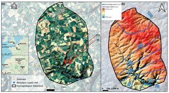
Figure 1.
(a) Location of the Limesy hydrogeological watershed, including the Becquigny supply well (blue), 129 mapped sinkholes (orange), and the two tracer-confirmed sinkholes (95 and 122) hydraulically connected to the supply well (red). (b) Groundwater table elevation (m a.s.l.) based on mean piezometric contours of the Chalk aquifer (2001–2006; BRGM Atlas, 2010), with DEM elevation derived from LiDAR measurements provided by IGN (m a.s.l.).
The catchment covers approximately 61 km2, with elevations ranging from 75 to 175 m a.s.l. The local geology consists of Upper Cretaceous Chalk (Cenomanian to Campanian) overlain by thick surficial deposits, predominantly clay-with-flints resulting from chalk weathering, with loess and Tertiary sands also present [12,34,35]. The overburden thickness ranges typically between 5 and 10 m. Regionally, groundwater recharge is expected to occur primarily through two pathways: rapid localized infiltration via sinkholes and karst conduits, and slower diffuse percolation through the surficial cover [3]. A recent survey mapped 117 sinkholes within the hydrogeological catchment, while a further 12 sinkholes located in the adjacent topographic watershed were also considered in this study (Figure 1). The climate is temperate oceanic, with a mean annual temperature of ~13 °C [11,36].
A major NW–SE-oriented structural lineament extends across the Saffimbec valley from Pavilly to Mesnil-Panneville. The Saffimbec valley corresponds to the main NW–SE-oriented valley visible in the south-western part of Figure 1b. This structure belongs to the complex fault system known as the “Seine Fault” and is associated with two other sub-parallel faults affecting the plateau south of the valley. Related to these major structural features, numerous fractures and secondary faults may have contributed to the development of karst formations within the Chalk, expressed at the surface by infiltration features such as dry valleys and sinkholes. However, the exact geometry of the karst system remains poorly characterized.
In Figure 1b, the regional groundwater elevation in the Chalk, estimated from large-scale interpolation of sparse measurements provided by BRGM, indicates a general groundwater flow direction from NW to SE. Across the catchment, the groundwater table ranges from slightly above 130 m a.s.l. to slightly below 80 m a.s.l. In comparison with the DEM, the groundwater depth reaches a maximum of around 40 m beneath the northern plateau and decreases to about 5–10 m in the southern valley. Sinkholes are predominantly located in the valleys (Figure 1a). Consequently, the vertical distance between sinkholes and the underlying karst drainage network is likely relatively small.
3. Methodology
3.1. WaterSed
WaterSed is an expert GIS raster-based distributed model that simulates catchment-scale runoff and soil-erosion patterns at the scale of individual rainfall events. As an upgraded version of STREAM [9,37], WaterSed represents each DEM cell as a reservoir, computes water and sediment budgets, and routes them through the surface flow network.
To compute runoff and erosion for any location in the catchment, WaterSed requires (i) a hydrologically conditioned DEM (using IGN RGE ALTI 5 m from BD ALTI ®), from which slope and the flow network are computed after depression filling to ensure a continuous downslope gradient [38]. (ii) A stream network and channel widths (using hydrographic network from BD TOPAGE®/BD Carthage®; channel widths from BD TOPO® and field surveys), which are used to define the drainage topology. Following the pre-processing, the stream network was corrected and refined based on on-site field observations. (iii) Land-cover (using the French Land Parcel Identification System (RPG)) and soil-texture maps (using RRP Haute-Normandie (Référence Régional Pédologique)) harmonized into classes of surface-sealing susceptibility. (iv) Expert-based decision tables adapted to local conditions, which associate each combination of land cover, soil texture, vegetation cover, surface crusting, and surface roughness with a set of hydrological and erosion parameters (steady-state infiltration capacity, Manning’s roughness coefficient, potential suspended-sediment concentration, and soil erodibility) following the expert-based matching approach developed for loess soils susceptible to crusting [10,37,39,40], converted into spatially distributed model parameters using the PREMACHE property tables [41]. (v) Rainfall events, such as only those with a total precipitation ≥ 2 mm that are considered in this study, antecedent moisture (rainfall during the previous 48 h), effective rainfall duration, and maximum rainfall intensity.
The outputs generated by WaterSed are then used as input variables in the deep learning models described in the following section.
3.2. Deep Learning Models
The deep learning architectures considered in this study rely on different approaches to capture temporal dependencies in sequential data to model turbidity at the supply well. CNN-based models learn local temporal patterns through convolutional filters, whereas LSTMs model sequential dependencies that use gated memory units. Hybrid CNN/LSTM architectures combine these mechanisms by first extracting short-term features with convolutional layers and then capturing longer-term dynamics through recurrent units. TCNs provide a convolutional alternative to recurrent models by using dilated causal convolutions. Time2Vec embeddings enrich the input by introducing a learnable encoding of temporal signals, including both periodic and non-periodic components, which is then processed by convolutional layers. These architectures were compared within the same modeling pipeline to identify the model that best reproduces turbidity dynamics in karst systems.
3.2.1. CNN, BiLSTM and Hybride CNN LSTM
We implemented an Optuna-based pipeline that explores three deep learning model families to identify the model achieving the best validation performance. The search space includes CNN (Convolutional Neural Networks), LSTM (Long Short-Term Memory networks), and hybrid CNN/LSTM configurations.
CNNs are composed of convolutional and pooling layers that apply filters to extract structured patterns from input data. They are followed by fully connected layers which aggregate features for a task-specific latent temporal representation which captures trends, seasonality, and lagged dependencies [20]. LSTMs [21] are a type of recurrent neural network build with gating mechanisms (input, forget, output) that decide what to keep from the past, what to write from the present, and what to expose to the next step, enabling the capture of short- and long-term dependencies in sequential data.
A hybrid CNN/LSTM architecture leverages the strengths of both models for time-series forecasting. CNN layers extract local patterns across time, while the LSTM captures short- and long-term temporal dependencies through gated memory units. The combination enables the model to learn local temporal features and sequential dynamics before producing the final forecast [22,23,24,25].
3.2.2. TCN
A TCN is a one-dimensional fully convolutional model built from causal and dilated convolutional layers with residual connections [26]. Causality ensures that the model does not use future information, while dilations enlarge the receptive field efficiently and residual connections help stabilize optimization [26]. TCNs have shown strong performance for sequence modeling and hydrological forecasting, including groundwater-level prediction with low computational cost [28], advance prediction in coastal aquifers [29], and runoff forecasting when combined with an Encoder–Decoder framework [27].
3.2.3. Time2Vec CNN
Prior work shows that Time2Vec, a learnable temporal encoding layer, can help forecast both periodic and non-periodic behaviors, improving robustness across time ranges [31]. We therefore add a learnable Time2Vec embedding of a normalized time scalar to each input window. At every step, Time2Vec provides one learned linear term plus several learned sinusoidal terms (with trainable frequencies and phases), giving an explicit temporal representation [30]. We then concatenate these time embeddings with the WaterSed-derived features, and process the resulting sequence using 1D convolutional CNN layers to extract local temporal patterns.
3.3. Modeling Pipeline and Performance
To avoid any data leakage, the dataset was split into a training and a test set prior to training and hyperparameter search. The dataset was split chronologically using 1 October 2022 as the separation date, resulting in 86.4% of the observations used for training and hyperparameter optimization and 13.6% reserved for testing. The test set was kept exclusively for final evaluation. Model training and optimization were conducted on the training set using both normalized (Min–Max scaler between 0 and 1) inputs to facilitate optimization, and raw inputs in order to preserve model weight information for the later interpretability analyses.
Models were optimized with Optuna [32] using the Tree-structured Parzen Estimator (TPE) sampler, an adaptive Bayesian optimization method. The deep learning models were implemented using PyTorch, an open-source deep learning framework widely used for neural network development. To ensure generalization while preserving temporal causality, we used a folded time-series cross-validation scheme (TimeSeriesSplit). Preliminary tests showed that three to four folds provided the most stable performance while also reducing computational cost. Several loss functions were evaluated (MSE, MAE, and a weighted MAE designed to emphasize turbidity peaks through a penalty applied above a predefined threshold). For each fold, models were trained for a fixed number of epochs with model checkpointing to retain the epoch with the lowest validation loss. The mean validation loss across folds served as the optimization objective.
After optimization, model performance was evaluated using a combination of global metrics computed on the continuous turbidity signal (MSE, RMSE, MAE, and Kling–Gupta Efficiency (KGE)) and event-based metrics specifically targeting turbidity peaks exceeding 30 NTU, a threshold chosen to separate background variability from distinct turbidity events at the studied water supply well. Peak detection performance was quantified using the probability of detection (POD) and the false alarm ratio (FAR), while peak amplitude accuracy was evaluated on matched peaks using RMSE, MAE, and Kling–Gupta Efficiency (KGE). KGE was preferred over Nash–Sutcliffe Efficiency (NSE) because it jointly captures correlation, bias, and relative variability between observed and simulated turbidity [19].
To accelerate the search, we adopted a two-stage optimization strategy with an initial coarse exploration using large batch sizes and short training runs, followed by a refined optimization restricted to the best-performing architectures using smaller batch sizes and longer training budgets. Although the number and nature of hyperparameters varied across model families, we maintained as many consistent settings as possible and explored a wide hyperparameter range for the CNN, LSTM, and hybrid CNN/LSTM architectures to capture performance trends.
3.4. Captum Interpretability
We interpreted the internal behavior of the deep learning models using Captum, a model interpretability library designed for PyTorch that provides attribution methods for neural networks.
Two gradient-based techniques were applied; Integrated Gradients (IG) and DeepLiftShap (DLS). IG estimates contributions by integrating gradients along a path from a baseline to the input, whereas DLS uses a SHAP-inspired multi-baseline approach to account for non-linear effects. Using both methods provide complementary perspectives and improves the robustness of the interpretability results.
4. Data
4.1. WaterSed Data
The WaterSed modeling period was selected to match the time interval over which turbidity measurements are the most reliable and to coincide with the beginning of the local agricultural calendar in August. Accordingly, the simulations were conducted from 5 August 2019 to 31 March 2023, corresponding to a total duration of 1335 days.
Rainfall data were obtained from the Météo-France rain gauge station of Éctot-lès-Baons, France, located approximately at 2.5 km from the studied catchment. Given the proximity of the station and the small size of the watershed, these data were considered representative of the hydroclimatic conditions over the study area.
Over this period, only hydroclimatic events with daily precipitation P > 2 mm·d−1 were modeled, resulting in 354 rainfall events used as inputs to the WaterSed model. Days with precipitation below this threshold (P < 2 mm·d−1) were assigned zero hydroclimatic values in order to reduce computational cost. However, to preserve information related to antecedent wetness conditions, we included the variable Rainfall depth over the previous two days (mm) (Figure 2b), which acts as a hydroclimatic memory effect. When the variable Rainfall depth over the two previous days (mm) is non-zero (e.g., due to accumulated rainfall over preceding days), its values range from 0.2 mm to 58.1 mm. The rainfall associated with modeled events (hereafter referred to as rainfall depth) ranges from 2 mm, according to the selected threshold, to a maximum of 42.8 mm, with a mean of 9.3 mm (Figure 2d). Some hydroclimatic events extend over two consecutive days. The effective rainfall duration (Figure 2c) varies from 18 to 990 min, with a mean duration of 173 min for events with P > 2 mm·d−1. Maximum rainfall intensity (mm·h−1), also used as an input variable due to its relevance for short-term erosion processes, ranges from 2 to 105 mm·h−1, with a mean intensity of 11.95 mm·h−1 (Figure 2a). All hydroclimatic variables described above were used both as inputs to the WaterSed model and as predictors in the deep learning framework.
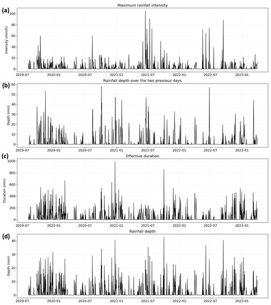
Figure 2.
Hydroclimatic time series used as inputs to the WaterSed model and the deep learning models over the study period (2019–2023); (a) maximum rainfall intensity (mm·h−1), (b) cumulative rainfall depth over the two preceding days (mm), (c) effective rainfall duration (min), and (d) daily rainfall depth (mm).
A key strength of the WaterSed model is its representation of cropping calendars, which enables the simulation of seasonal variations in soil surface conditions that control runoff and erosion processes. Based on land-use and soil-texture information derived from national databases (RPG and RRP), land-use classes were associated with monthly soil surface states using decision tables adapted to local conditions. These tables describe the temporal evolution of vegetation cover, surface roughness, and soil surface crusting for each crop class, following established cropping calendars [36,39].
Figure 3 below represents the modal crop type per parcel over the period 2019 to 2023. The modal land-use distribution over the 2019–2023 period is dominated by flax (33.58%), followed by vegetated areas including forests and green spaces (16.69%), permanent grasslands (14.31%), maize (10.87%), potatoes (9.67%), and impervious surfaces such as roads and parking areas (7.29%). Rapeseed accounts for 4.22% of the area, while minor land-use classes include runoff axes (1.29%), unpaved roads and railways (0.90%), sugar beet (0.66%), wheat (0.27%), orchards (0.22%), water bodies (0.03%) and construction sites (0.01%).
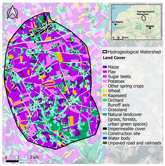
Figure 3.
Modal land-use distribution over the 2019 to 2023 period on the Limesy WaterShed.
4.2. Turbidity Data
Turbidity was measured using a nephelometer at the Bécquigny drinking-water supply from 1 June 2010 to 31 March 2023. Raw turbidity data consist of a time series recorded at a 5 min sampling interval. As the objective of this study is to forecast turbidity peaks, daily maximum turbidity values were extracted from the raw time series. The resulting dataset consists of a daily maximum turbidity time series (Figure 4a).
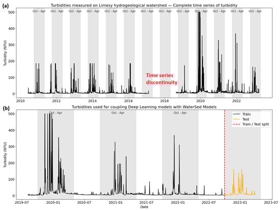
Figure 4.
(a) Reconstructed daily turbidity (NTU) measured at the Becquigny supply well over the 2010 to 2023 period. (b) Reconstructed daily turbidity (NTU) extracted after the time-series discontinuity and used for coupling deep learning models with WaterSed simulations.
A data gap is observed between 16 February 2017 and 18 August 2018, corresponding to the replacement of the nephelometer with a newer one.
Between 2010 and 2017, turbidity was measured using the former nephelometer, which imposed an upper measurement limit, resulting in turbidity peaks capped at approximately 180–190 NTU. After the instrument was replaced in 2018, the new nephelometer allowed higher values to be recorded, with maximum turbidity reaching up to 500 NTU, consistent with its extended measurement range.
In the following analyses, only data from the 2018–2023 period are used (Figure 4b), as they are both more recent and more reliable. Over this period, turbidity data are missing for only 16 days; these missing values were estimated using the global median of the daily turbidity time series.
The turbidity data presented in Figure 4b correspond to the target variable used in our deep learning model. The separation date between the training and test periods was set to 1 October 2022. The training period extends from 5 August 2019 to 30 September 2022 and comprises 1153 days, while the test period covers 1 October 2022 to 31 March 2023, corresponding to 182 days.
During the training period, the maximum observed turbidity reaches 500 NTU. Using 30 NTU as a reference threshold to separate background variability from distinct turbidity events at the studied water supply well, the training period includes 164 days exceeding this threshold, representing 10.75% of the training days. During the test period, the maximum turbidity reaches 164 NTU, with 26 days exceeding 30 NTU, corresponding to 14.29% of the test days.
Figure 4a,b show that turbidity peaks consistently occur between October and April. As our primary objective is to forecast turbidity peaks, we constructed a secondary dataset evaluated in the following section. This second dataset consists of data from 2018 to 2023, restricted to the October to April period of each year. Our working hypothesis is that training the models on data concentrated during peak months may reduce noise and improve predictive performance. This choice was made to concentrate the training data on periods with a higher occurrence of turbidity peaks, thus reducing the dominance of long periods with low turbidity variability in the training process.
4.3. Tracer Test Data: Historical Transfer Time
Two hydrogeological tracer test campaigns involving five sinkholes within the hydrogeological watershed feeding the Becquigny supply well were conducted. Of these five sinkholes, only two showed a positive tracer detection. Table 1 summarizes the characteristics of these two tests, including tracer type, distance to the supply well, and first arrival time.

Table 1.
Summary of positive tracer test results between injection sinkholes and the supply well.
According to Table 1, the two sinkholes with positive tracer detection are located at 3.0 km and 2.6 km from the Becquigny supply well. First arrival times ranged from 9 h 50 min (sinkhole 122, Tinopal) to 16 h 00 (sinkhole 95, Sulforhodamine B), indicating rapid karstic transfer.
Tracer detection was first identified using a GGUN FL-24 field fluorimeter installed at the pumping well. The arrival of both tracers was confirmed by automatic samplers. Tracer injections consisted of 8 kg of Tinopal at sinkhole 122 and 4 kg of Sulforhodamine B at sinkhole 95. Laboratory analyses of the collected samples revealed peak concentrations of approximately 14.9 ppb for Tinopal and up to 64.1 ppb for Sulforhodamine B. These results confirm the existence of hydraulic connections between the injection sinkholes and the supply well.
During the tracer tests, high background turbidity in the pumped water generated noise in the measured signal, which introduced some uncertainty in the exact determination of the first arrival times. However, the combined evidence from GGUN FL-24 monitoring and laboratory analyses confirms rapid hydraulic transfer between the tested sinkholes and the Becquigny supply well.
The relatively short travel times observed here suggest efficient transport through preferential pathways (karstic conduit).
By visual inspection of the site map in Figure 1, these two sinkholes are also among the closest features to the intake, suggesting a preferential flow connectivity to the supply well.
5. Results
5.1. WaterSed Results
The outputs of the WaterSed model consist of raster datasets produced at the scale of the hydrogeological catchment. Spatial raster of runoff and sediment discharge are generated for each rainfall event. These variables are then extracted at the locations of the 129 identified sinkholes (see Figure 1). Because the activity of individual sinkholes is temporally variable and runoff pathways may evolve over time, we adopt the working hypothesis that runoff and sediment fluxes entering a sinkhole are conserved downstream at the catchment scale. Figure 5 presents the time series of sediment discharge (Figure 5a) and runoff (Figure 5b) aggregated over the 129 sinkholes, as well as their cumulative values over the study period (Figure 5c).
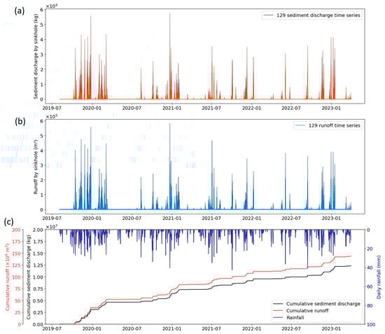
Figure 5.
(a) Sediment discharge time series simulated by WaterSed for the 129 sinkholes of the Limésy hydrogeological watershed over the study period, (b) runoff time series simulated by WaterSed for the same 129 sinkholes, (c) cumulative sediment discharge and cumulative runoff at the catchment scale and measured turbidity time series at the supply well over the study period.
Under the assumption that runoff and sediment discharge are conserved downstream, the maximum sediment discharge reaches 57.59 t d−1 and the maximum runoff reaches 5.82 × 10⁵ m3 d−1. Both maxima are associated with a single sinkhole (sinkhole no. 30). However, as shown by the ranked cumulative runoff contributions and ranked cumulative sediment discharge presented in Appendix A, sinkhole no. 30 exhibits a numerical artifact. Despite this issue, sinkhole no. 30 is retained in the deep learning models, as the modeling framework is able to filter out and mitigate such artifacts. Excluding this sinkhole, the highest modeled sediment discharge is 29.63 t d−1, and the highest runoff is approximately 3.13 × 10⁵ m3 d−1.
Figure 5c shows that cumulative runoff and cumulative sediment discharge predominantly increase between October and April, reflecting a seasonality in the hydrosedimentary transfer. By contrast, the rainfall events that occurred during the summer of 2021, showing a marked increase in both cumulative runoff and cumulative sediment discharge, did not generate significant turbidity peaks at the supply well. This decoupling highlights that important rainfall, high runoff and sediment discharge do not systematically translate into turbidity responses, particularly during summer conditions. This observation indicates that surface processes alone are insufficient to explain turbidity dynamics at the supply well, and that seasonal (hydrogeological) conditions impact the connectivity and transfer of suspended sediments through the karst system. Consequently, to improve the performance of our deep learning models, a seasonal covariate was introduced in our models in order to constrain the learning process and better account for seasonal controls on turbidity dynamics at the supply well.
5.2. Deep Learning Results
In the following section, the objective of the deep learning approach is not to maximize predictive performance through an optimized selection of input data, but rather to assess the relative contribution of individual sinkholes to turbidity peaks observed at the supply well.
The inputs of the deep learning models consist of four hydroclimatic variables (Figure 2), one seasonal static covariate, and 129 sediment discharge time series (Figure 5a) together with 129 runoff time series (Figure 5b), corresponding to one sediment and one runoff signal per sinkhole. Consequently, turbidity values at the supply well are predicted using a total of 263 covariates. No sinkhole specific feature selection was applied to optimize model performance, and all sinkholes were retained, including sinkhole 30, which is affected by a numerical artifact.
Figure 6a,b illustrate the first optimization stage, in which hybrid CNN/LSTM, Time2Vec-CNN, and TCN architectures were trained using comparable hyperparameter ranges, the same number of epochs (1000), identical train–validation splits, and an equal number of Optuna trials (1000). Figure 6a shows results on the training period, while Figure 6b presents the corresponding results on the test period. For each architecture, the optimization was conducted using MAE, MSE, or weighted MAE loss functions, both with and without normalization, and additionally using a secondary dataset restricted to the October–April period. This experimental design resulted in 72 trained models, of which 70 are displayed in Figure 6a,b, as two runs failed during training.
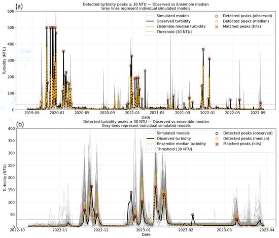
Figure 6.
(a) Summary of the 70 deep learning models over the training period; gray lines correspond to the best-performing model selected after 1000 Optuna trials for each model configuration. The ensemble median turbidity is shown solely to illustrate the peak detection method above the 30 NTU threshold. (b) Summary of the same 70 deep learning models over the testing period; gray lines correspond to the best-performing model selected after 1000 Optuna trials for each model configuration. The ensemble median turbidity is shown solely to illustrate the peak detection method above the 30 NTU threshold.
The performance metrics reported in Table 2 were used to evaluate each individual model from the first optimization stage. For visualization purposes only, the same evaluation framework was applied to the median performance of each model distribution in Figure 6a,b. Based on these results, fourteen models were selected for a second refined optimization, conducted with a reduced batch size and 3000 Optuna trials. The best-performing model resulting from this second optimization was then selected for the interpretability analysis.
Table 2.
Summary of the same 70 deep learning models over the testing period; gray lines correspond to the best-performing model selected after 1000 Optuna trials for each model configuration. Metrics are reported as mean ± standard deviation across models, reflecting inter-model variability. The ensemble median turbidity is shown solely to illustrate the peak detection method above the 30 NTU threshold.
In Table 2, performance metrics of the second optimization shows an improvement in model generalization. Compared to the first optimization, tested RMSE and MAE on the continuous turbidity signal decrease, while KGE values indicate a better balance between bias, variability, and temporal dynamics. Peak-related performances are also enhanced, with a reduction in false alarm rates and improved peak amplitude errors. Although peak KGE values remain moderate, the results demonstrate a more reliable detection and quantification of turbidity peaks, consistent with the study’s interpretability-oriented objective rather than pure predictive optimization.
The best resulting model (Figure 7) after optimization 2 was further refined by introducing validation split, early stopping and model checkpointing in order to limit overfitting and maximize predictive performance. The optimal architecture corresponds to a CNN/LSTM model composed of two CNN layers and two LSTM layers, with a sequence length of 8 days and a CNN kernel size of 2. The most effective configuration relies on the MAE loss function, trained on normalized inputs and using the full dataset, without restricting the secondary dataset to the October–April period. The best prediction is found at 23 epochs (while the optimization was conducted on 75 epochs).
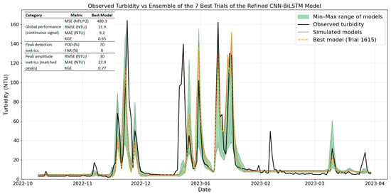
Figure 7.
Observed turbidity compared with the best-performing CNN–BiLSTM model after two successive optimization stages and the ensemble of the seven best Optuna trials. The dashed orange line shows the selected and refined best model, while the green shaded area highlights inter-model agreement rather than uncertainty.
Compared to the test results obtained during the two optimization stages, the best model shows a clear and consistent improvement across all evaluation metrics, as reported in the performance summary table embedded in Figure 7. Global performance on the continuous signal is enhanced with the RMSE reduced from 34.8 ± 10.1 NTU (optimization 1 test) and 28.5 ± 6.1 NTU (optimization 2 test) to 21.9 NTU, and the MAE decreasing to 9.2 NTU. The KGE increases to 0.65, indicating a markedly improved agreement in terms of correlation, bias, and variability. Peak detection skill remains robust (POD = 70%), while false alarms are completely eliminated (FAR = 0%). The largest gains are observed for peak amplitudes, with RMSE and MAE on matched peaks reduced to 30 NTU and 27.9 NTU, respectively, and a peak KGE of 0.77, compared to near-zero or negative values during both optimization tests.
It is worth noting that two turbidity peaks are systematically missed by all model configurations. These two events have different origins. The December peak coincides with variations in other meteorological variables not used in our model (see Appendix B), suggesting that broader hydrometeorological conditions may have contributed to this event. The smaller peak observed in February cannot be associated with any identifiable meteorological signal in either the local dataset or the additional meteorological variables analyzed. This suggests that the event may be driven by other transport processes, such as intra-karst sediment remobilization or direct sediment transfer not represented by the available covariates, or by unidentified processes (e.g., human disturbance or measurement error).
5.3. Interpretability Results
Building on the best-performing hybrid CNN/LSTM model identified in the previous section, interpretability analyses were conducted to quantify the contribution of individual inputs to turbidity predictions. Global importance was compared using Integrated Gradients and DeepLiftShap. DeepLiftShap was retained for analyses, as it provides stable and computationally efficient attributions in deep neural networks, while remaining grounded in DeepLIFT [42] and SHAP-inspired attribution principles.
In Figure 8, global feature importance was estimated by aggregating the absolute attribution values obtained with Integrated Gradients and DeepLiftShap. Although differences in relative importance are observed for secondary features, both methods show consistent dominant trends. This consistency indicates that the identification of the main controlling variables is not strongly sensitive to the choice of attribution method, supporting the robustness of the interpretation. Global importance results show that turbidity is primarily controlled by seasonal forcing and short-term rainfall accumulation (2 days before), while sediment discharge and runoff from multiple sinkholes contribute jointly at lower individual levels.
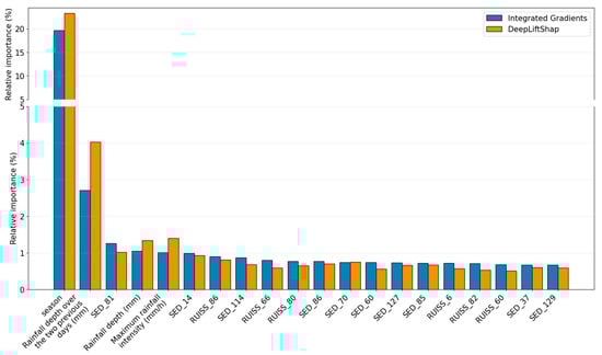
Figure 8.
Comparison of feature importance rankings obtained using Integrated Gradients and DeepLiftShap for the top 20 input variables of the best-performing CNN–LSTM model.
In contrast to global importance, which reflects average influence across the dataset, temporal attributions describe how and when individual variables contribute to turbidity predictions. Figure 9 presents the median and interquartile range of DeepLiftShap attributions for rainfall depth and the five most influential sinkhole variables as a function of time lag n (where t − n denotes the input value n days before the prediction time t). Temporal attributions indicate how and when each input variable provides predictive information used by the model to estimate turbidity at time t. A positive attribution at a given time lag indicates that higher values of this variable at that lag increase the predicted turbidity and a negative attribution indicates an attenuating effect.
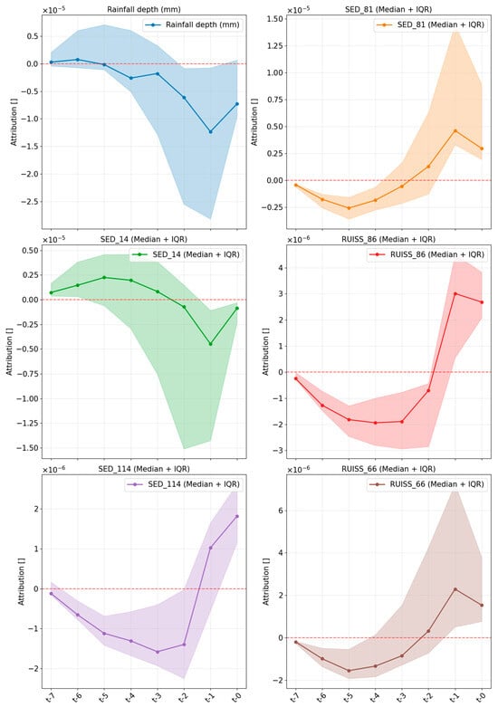
Figure 9.
Temporal attributions derived from DeepLiftShap for the rainfall depth and the five most influential sinkhole-related variables identified in the global importance analysis using the median and interquartile range.
In Figure 9, for most of the sinkhole-related variables, positive attributions are observed at short time lags (t–0 to t–2), indicating that recent sediment discharge and runoff provide the most informative signal for turbidity peak prediction, although the timing of the maximum contribution differs between sinkholes. At longer time lags, attributions tend to become negative, suggesting a dominant attenuation or recession effect in the model response.
SED_14 shows a distinct temporal attribution pattern compared to the other sinkholes, which is consistent with its location downstream of a pond and may suggest a buffering effect that modifies the timing of sediment transfer.
Rainfall depth shows predominantly negative contributions at short time lags, consistent with a dilution effect during peak development, while contributions approach positive values at longer lags, potentially reflecting antecedent conditions such as soil wetting rather than direct turbidity generation.
In Figure 10, the same method is applied to sinkhole 122 and sinkhole 95, on which we conducted the field tracer test and obtained positive results (cf. Figure 1).
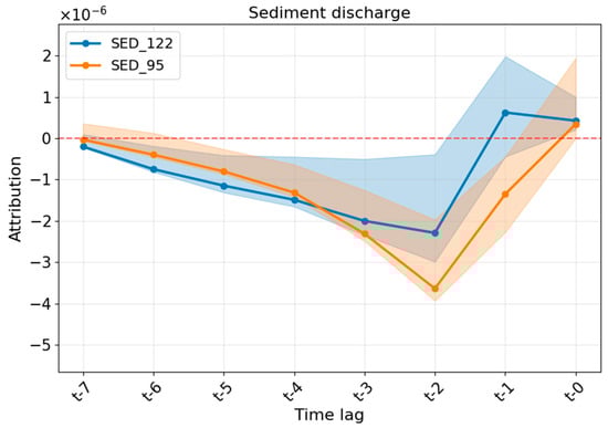
Figure 10.
Temporal attributions derived from DeepLiftShap for the two sinkholes with positive tracer test.
The temporal attributions for sinkholes 122 and 95 show positive sediment discharge contributions at t−0 for both sinkholes, consistent with tracer test results indicating transfer times shorter than one day at the daily scale. While the model captures sediment contributions within the correct transfer-time window, the daily resolution of the dataset and the model prevents direct comparison with tracer-derived transfer times at sub-daily time scales.
6. Discussion
The cascade modeling approach developed in this study extends the work of [12] by combining an expert-based GIS model with deep learning models to represent surface and subsurface sediment transfer in a karst environment. While the original cascade approach relied exclusively on sinkholes with positive tracer test responses, we inverted the pipeline by integrating all referenced sinkholes as potential contributors. This choice makes the WaterSed outputs particularly sensitive to noise and uncertainty in the input data. More generally, deep learning approaches in the hydrological sciences are known to be sensitive to data quality, noise, and uncertainty in input variables [12,43].
Despite this increased sensitivity, our WaterSed results remain robust and consistent with previous studies that used the same modeling framework [11,12]. A single modeling artifact was identified for sinkhole 30. However, our deep learning models were able to detect and disregard this artifact, demonstrating the robustness of the approach and its capacity to mitigate the influence of noisy or erroneous inputs.
The runoff and sediment fluxes simulated by WaterSed and extracted at sinkhole locations rely on the assumption that fluxes entering a sinkhole are conserved downstream. This assumption is a practical simplification. Because the activity of individual sinkholes is temporally variable and runoff pathways may evolve over time, the exact routing of runoff and sediment through each sinkhole cannot be directly quantified without extensive instrumentation at each individual sinkhole. Such monitoring is impractical in karst catchments characterized by numerous sinkholes and would become even less feasible when the methodology is upscaled to larger watersheds. However, these variables provide a consistent representation of runoff and sediment inputs to the karst system, allowing the deep learning model to capture the dominant dynamics controlling turbidity peaks at the supply well.
The main data quality limitation concerns the turbidity target series, as erroneous or misidentified values (e.g., driven by anthropogenic disturbances or processes unrelated to the studied hydrosedimentary transfers) directly bias the learning process and degrade predictive skill, and therefore are not predictable using our data. Despite this limitation, our best model achieves strong predictive performance, particularly with respect to turbidity peaks which constitute the primary objective of this study. On the test dataset, accuracy on the continuous turbidity signal remains high (RMSE = 21.9 NTU, MAE = 9.2 NTU, KGE = 0.65). The model also demonstrates robust peak detection (POD = 70%, FAR = 0%) and accurate peak amplitude reproduction (peak RMSE = 30 NTU, peak MAE = 27.9 NTU, peak KGE = 0.77). The obtained KGE values are comparable to those reported in recent deep learning studies using informative explanatory covariates [19].
These relatively strong model performances reflect the hydrogeological configuration of the study area. As shown by the piezometric data and topographic analysis in Figure 1b, many sinkholes are located in valley bottoms where the groundwater table is shallow. In these areas, the vertical distance between surface infiltration points and the underlying karst drainage network is likely limited. This configuration may favor direct and rapid hydrosedimentary transfers from sinkholes to the karst conduits, with reduced storage or attenuation within the epi-karst or secondary fracture network. Such conditions are consistent with the ability of the model to reproduce turbidity peaks with relatively high accuracy.
Beyond the predictive performance of our models, the interpretability analysis provides additional insight into the respective role of hydroclimatic and sinkhole-related variables. The application of interpretability techniques to machine learning models in hydrology and hydrogeology remains recent [44]. Most existing studies using machine learning interpretability focus on the use of climatic variables to predict groundwater levels [19,44,45] or discharge in karst systems [46].
Consistent with the findings of [47] for suspended-sediment concentration, our global importance analysis shows that variables describing the general hydrometeorological context are among the dominant contributors to turbidity predictions. In particular, seasonality and cumulative rainfall depth over the two preceding days emerge as key drivers, suggesting that the model primarily integrates information related to the initial state of the system, including seasonal conditions and antecedent wetness, before accounting for more localized inputs. The prominence of these seasonal controls is consistent with numerous previous studies on surface erosion processes, which have highlighted the strong seasonal modulation of sediment production and mobilization (e.g., [48]).
In the present study, sediment discharge variables associated with sinkholes (e.g., SED_81, SED_14, SED_114) and runoff-related indices (RUISS_86, RUISS_66) exhibit intermediate but consistent importance levels. None of these variables dominate individually; instead, they form a set of complementary signals reflecting the spatial heterogeneity of sediment discharge and runoff contributions across the catchment. This indicates that, in the Limésy watershed, turbidity predictions emerge from the combined influence of multiple sinkholes rather than from a single or few dominant sources. The absence of a single dominant sinkhole across the catchment reflects the spatially heterogeneous recharge structure typical of well-developed karst systems, where numerous sinkholes act as localized recharge points and groundwater circulation occurs through multiple preferential pathways rather than through a single dominant conduit.
In addition to identifying the most influential predictors, the temporal attribution analysis also helps characterize the response dynamics of the karst system. While several methodological studies have proposed and validated attribution frameworks explicitly designed for time series and sequential models, such as KernelSHAP for time-series classification [49] and TimeSHAP for recurrent architectures [50], only a limited number of applied studies have adopted lag-based attribution analyses in environmental sciences. Recent examples in hydrology illustrate this emerging practice in the context of explainable machine learning applied to reservoir forecasting and hydrometeorological influence analysis (e.g., [51,52]). To our knowledge, no previous study has applied a methodology based on the aggregation of SHAP attributions as a function of temporal lag within the input sequence to a cascade modeling framework combining process-based hydrological outputs and deep learning predictions in karst.
Temporal attribution patterns from our model reveal a strong concentration of positive contributions at short time lags (t-0 to t-2) for most sinkholes with related sediment discharge and runoff variables. These short time lag attributions indicate that recent surface runoff and sediment discharge entering the karst through sinkholes are the primary drivers of turbidity peaks, reflecting a rapid and event-driven karst response characteristic of well-developed and reactive karst systems. The timing of maximum attribution varies between sinkholes, highlighting heterogeneity in effective response timing, transfer efficiency, and local connectivity within the karst network. These differences may reflect variations in several hydrogeological factors, including the distance to the supply well, land-use conditions controlling sediment production at the surface, and the structure of karstic flow pathways. In this regard, the attribution analysis provides a way to identify potential sediment sources and sediment sinks within the karst system and to characterize their temporal dynamics.
This short time scale and event-driven turbidity response is consistent with previous studies on turbidity dynamics in karst systems [53,54,55]. These results indicate that the deep learning model does not only achieve predictive skill but also captures key hydrogeological controls of the karst system, including rapid conduit transfer, heterogeneous sinkhole connectivity, and short-term event-driven sediment transport.
At longer time lags, attributions systematically shift toward negative values, indicating attenuation and recession effects. This transition highlights the absence of effective sediment inputs in the days preceding the turbidity peak which indicates that sediment discharge occurring several days before the event does not contribute to peak turbidity development.
Such behavior, characterized by short-time-scale amplification, is typical of reactive karst systems and has been widely documented [53,54,55].
One sinkhole (SED_14) exhibits a slightly different temporal attribution pattern, with contributions that are more distributed over time. This behavior is noteworthy given its location downstream of a pond and suggests a hydrological buffering effect associated with temporary surface storage, which may delay or drastically reduce sediment transfer and smooth short-term responses compared to more directly connected sinkholes.
Rainfall depth exhibits a distinct temporal signature, with predominantly negative attributions at short time lags, consistent with dilution during peak development, and weakly positive contributions at longer lags. This pattern suggests that rainfall primarily modulates turbidity indirectly, through antecedent wetness and runoff generation potential, rather than acting as a direct driver of sediment input at the event scale.
These attribution patterns are further supported by the tracer test results. The analysis of sinkholes 122 and 95, which have shown positive responses during field tracer tests conducted during our study, reveals positive sediment discharge attributions at t-0, consistent with transfer times shorter than one day. The three other negative tracer tests indicate that these sinkholes are not directly connected to the Becquigny supply well, or that the tracers were conducted toward other outlets of the karst system. These negative results highlight the spatial heterogeneity of hydraulic connections within the karst system. Although the daily temporal resolution of the model prevents resolving sub-daily differences observed in tracer experiments, the agreement in attribution timing confirms that the model captures the correct transfer-time window for hydraulically connected sinkholes. This consistency supports the physical relevance of the learned relationships and indicates that the model internalizes key transport processes of a reactive karst system.
This result is particularly promising, as higher temporal resolution simulations over multi-year periods were not feasible here due to computational constraints. Applying this methodology to watersheds characterized by longer transfer times, or to modeling frameworks operating at hourly time steps, could provide a much more detailed understanding of karst flow pathways and internal circulation dynamics in karstic environments.
Further evaluation of this framework in larger watersheds where numerous sinkholes have been investigated through tracer tests and where greater variability exists in geological settings, land use, and transfer distances would provide valuable insights into the mechanisms controlling attribution differences between sinkholes. Such datasets would allow a direct comparison between attribution patterns inferred by the model and physically observed transport dynamics. In this context, the proposed framework could provide a promising basis for the development of physics-informed neural network approaches in karst hydrogeology, where model attributions may help constrain physically meaningful transfer times within the karstic network.
7. Conclusions
This study advances previous approaches coupling WaterSed outputs with deep learning by enabling the prioritization of sinkholes according to their contribution to turbidity peaks and by providing time-lagged information on sediment transfer within the karst network.
After multiple optimization rounds across several neural network architectures, our best-performing hybrid CNN-LSTM model achieved strong predictive performance in particular for turbidity peaks (KGE = 0.65 for the continuous signal and 0.77 for peak values). Our explainability analyses have shown that turbidity dynamics are primarily controlled by seasonal conditions and short-term rainfall accumulation, while sinkhole-related sediment discharge and runoff variables act as complementary drivers rather than as isolated dominant sources.
Temporal attributions reveal a characteristic karst response at the event scale, marked by rapid positive contributions at short time lags (t-0 day to t-2 days) followed by no-contribution at longer lags, which is consistent with reactive karst behavior. These results suggest that explainable deep learning may provide valuable insights into the effective timing and hydrosedimentary responses within karst networks.
The temporal attribution method is promising for application to larger karst networks and hydrogeological watersheds, where transfer pathways and transfer times are more variable. The availability of tracer-tested sinkholes with physically based transfer-time estimates would enable robust validation of temporal attribution estimation of derived transfer-time estimations. This approach may open the way toward large-scale characterization of karst connectivity and sediment transport processes.
Beyond the scope of the present study and based on sensitivity analyses of both WaterSed and deep learning models, additional WaterSed simulations incorporating mitigation measures provided estimates of the potential reduction in turbidity peaks associated with different management options. This modeling pipeline is currently being applied in collaboration with stakeholders to assess the potential impact of mitigation measures implemented at specific sinkholes.
By identifying the sinkholes contributing most to turbidity peaks, this approach allows us to identify those that require specific work to reduce the transfer of sediment from the surface to the drinking well. This is a helpful result for stakeholders to develop a water resource protection plan.
Author Contributions
Conceptualization, B.N. and M.F.; methodology, B.N. and M.F.; software, B.N.; validation, B.N.; formal analysis, B.N.; investigation, B.N.; resources, M.F.; data curation, B.N.; writing—original draft preparation, B.N. and M.G.; writing—review and editing, B.N., M.G., A.J., N.M. and M.F.; visualization, B.N. and M.G.; supervision, M.F.; project administration, A.J., N.M. and M.F.; funding acquisition, M.F. All authors have read and agreed to the published version of the manuscript.
Funding
This research was funded by the Seine-Normandy Water Agency, the BRGM, the AREAS, the syndicat of SERPN, the syndicat SIAEP du Lieuvin and the syndicat Caux-Austreberthe.
Data Availability Statement
The dataset used in this study is available following this link: https://doi.org/10.6084/m9.figshare.31375777.
Acknowledgments
We are grateful to the three anonymous reviewers for their valuable comments, which greatly improved the clarity and quality of this paper. We thank BRGM for providing the framework and technical guidance required to implement the WaterSed models. We also thank the SERPN, the SIAEP du Lieuvin, and the Caux-Austreberthe syndicate for supplying the data necessary to carry out this study. Finally, we acknowledge AREAS for conducting the initial processing of the turbidity data. Deep Learning models were built using PyTorch [56].
Conflicts of Interest
The authors declare no conflicts of interest. The funders had no role in the design of the study; in the collection, analyses, or interpretation of data; in the writing of the manuscript; or in the decision to publish the results.
Abbreviation
| DEM | Digital Elevation Model |
| ANN | Artificial Neural Network |
| LSTM | Long Short-Term Memory |
| CNN | Convolutional Neural Network |
| TCN | Temporal Convolutional Network |
| RPG | Registre Parcellaire Graphique (French Land Parcel Identification System) |
| RRP | Référence Régional Pédologique (French Soil Reference Database) |
| MSE | Mean Squared Error |
| MAE | Mean Absolute Error |
| RMSE | Root Mean Square Error |
| KGE | Kling–Gupta Efficiency |
| POD | Percentage Of Detection |
| FAR | False Alarm Ration |
| NSE | Nash–Sutcliffe Efficiency |
| IG | Integrated Gradient |
| DLS | DeepLiftShap |
Appendix A

Figure A1.
(a) Top 50 sinkholes by cumulative runoff contribution. (b) Top 50 sinkholes by cumulative runoff contribution, excluding sinkhole number 30. (c) Top 50 sinkholes by cumulative sediment discharge. (d) Top 50 sinkholes by cumulative sediment discharge, excluding sinkhole number 30.
Figure A1.
(a) Top 50 sinkholes by cumulative runoff contribution. (b) Top 50 sinkholes by cumulative runoff contribution, excluding sinkhole number 30. (c) Top 50 sinkholes by cumulative sediment discharge. (d) Top 50 sinkholes by cumulative sediment discharge, excluding sinkhole number 30.

Appendix B
Figure A2a,b reproduces the same WaterSed outputs presented in Figure 5, but restricted to the test period. The Figure A2c shows the positive part of the derivative of the SAFRAN variable DRAINC_Q, which represents drainage simulated by the Météo-France meteorological reanalysis [57]. Considering only the positive values of the derivative highlights periods of increasing drainage, corresponding to phases of system recharge or hydrological activation. The comparison with turbidity suggests that the December turbidity peak discussed in Section 5.2 (Deep Learning Results) coincides with a strong increase in this drainage signal, indicating that the event may be related to broader hydrometeorological conditions captured by SAFRAN but not included among the model covariates.

Figure A2.
Test period only. (a) Sediment discharge time series simulated by WaterSed for the 129 sinkholes of the Limésy hydrogeological watershed over the study period, (b) runoff time series simulated by WaterSed for the same 129 sinkholes; (c) derivative of DRAINC_Q (Safran) versus turbidity.
Figure A2.
Test period only. (a) Sediment discharge time series simulated by WaterSed for the 129 sinkholes of the Limésy hydrogeological watershed over the study period, (b) runoff time series simulated by WaterSed for the same 129 sinkholes; (c) derivative of DRAINC_Q (Safran) versus turbidity.

References
- Masséi, N.; Dupont, J.-P.; Rodet, J.; Laignel, B. Assessment of direct transfer and resuspension of particles during turbid floods. J. Hydrol. 2003, 275, 109–121. [Google Scholar] [CrossRef]
- Stevenson, M.; Bravo, C. Advanced turbidity prediction for operational water supply planning. Decis. Support Syst. 2019, 119, 72–84. [Google Scholar] [CrossRef]
- BRGM. Aménagement des Bétoires en Haute-Normandie—État de L’art et Préconisations de Bonnes Pratiques; Rapport RP-58795-FR; BRGM: Paris, France, 2010.
- Patault, E.; Ledun, J.; Landemaine, V.; Soulignac, A.; Richet, J.-B.; Fournier, M.; Ouvry, J.-F.; Cerdan, O.; Laignel, B. Analysis of off-site economic costs induced by runoff and soil erosion: Example of two areas in the northwestern European loess belt for the last two decades (Normandy, France). Land Use Policy 2021, 108, 105541. [Google Scholar] [CrossRef]
- Renard, K.G.; Freimund, J.R. Using monthly precipitation data to estimate the R factor in the revised USLE. J. Hydrol. 1994, 157, 287–306. [Google Scholar] [CrossRef]
- Verstraeten, G.; Prosser, I.P.; Fogarty, P. Predicting the spatial patterns of hillslope sediment delivery to river channels in the Murrumbidgee catchment, Australia. J. Hydrol. 2007, 334, 440–454. [Google Scholar] [CrossRef]
- Laflen, J.M.; Lane, L.J.; Foster, G.R. WEPP: A new generation of erosion prediction technology. J. Soil Water Conserv. 1991, 46, 34–38. [Google Scholar] [CrossRef]
- Takken, I.; Beuselinck, L.; Nachtergaele, J.; Govers, G.; Poesen, J.; Degraer, G. Spatial evaluation of a physically-based distributed erosion model (LISEM). Catena 1999, 37, 431–447. [Google Scholar] [CrossRef]
- Souchère, V.; King, D.; Daroussin, J.; Papy, F.; Capillon, A. Effects of tillage on runoff directions: Consequences on runoff contributing area within agricultural catchments. J. Hydrol. 1998, 206, 256–267. [Google Scholar] [CrossRef]
- Cerdan, O.; Le Bissonnais, Y.; Couturier, A.; Bourennane, H.; Souchère, V. Rill erosion on cultivated hillslopes during two extreme rainfall events in Normandy, France. Soil Tillage Res. 2002, 67, 99–108. [Google Scholar] [CrossRef]
- Landemaine, V.; Cerdan, O.; Grangeon, T.; Vandromme, R.; Laignel, B.; Evrard, O.; Salvador-Blanes, S.; Laceby, P. Saturation-excess overland flow in the European loess belt: An underestimated process? Int. Soil Water Conserv. Res. 2023, 11, 688–699. [Google Scholar] [CrossRef]
- Patault, E.; Landemaine, V.; Ledun, J.; Soulignac, A.; Fournier, M.; Ouvry, J.-F.; Cerdan, O.; Laignel, B. Simulating sediment discharge at water treatment plants under different land use scenarios using cascade modelling with an expert-based erosion-runoff model and a deep neural network. Hydrol. Earth Syst. Sci. 2021, 25, 6223–6238. [Google Scholar] [CrossRef]
- Savary, M.; Johannet, A.; Masséi, N.; Dupont, J.-P.; Hauchard, E. Operational Turbidity Forecast Using Both Recurrent and Feed-Forward Based Multilayer Perceptrons. In Advances in Time Series Analysis and Forecasting; Springer: Berlin/Heidelberg, Germany, 2017. [Google Scholar] [CrossRef]
- Jourde, H.; Massei, N.; Mazzilli, N.; Binet, S.; Batiot-Guilhe, C.; Labat, D.; Steinmann, M.; Bailly-Comte, V.; Seidel, J.-L.; Arfib, B.; et al. SNO KARST: A French Network of Observatories for the Multidisciplinary Study of Critical Zone Processes in Karst Watersheds and Aquifers. Vadose Zone J. 2018, 17, 180094. [Google Scholar] [CrossRef]
- Basu, B.; Morrissey, P.; Gill, L.W. Application of Nonlinear Time Series and Machine Learning Algorithms for Forecasting Groundwater Flooding in a Lowland Karst Area. Water Resour. Res. 2022, 58, e2021WR029576. [Google Scholar] [CrossRef]
- Zhou, Q.; Zhang, Y. Linear and nonlinear ensemble deep learning models for karst spring discharge forecasting. J. Hydrol. 2023, 624, 130394. [Google Scholar] [CrossRef]
- Zhou, R.; Zhang, Y.; Wang, Q.; Jin, A.; Shi, W. A hybrid self-adaptive DWT-WaveNet-LSTM deep learning architecture for karst spring forecasting. J. Hydrol. 2024, 634, 131128. [Google Scholar] [CrossRef]
- Janža, M.; Hudovernik, V.; Serianz, L.; Stroj, A. Modeling hydrological functioning of karst aquifer systems in Slovenia using geomorphological features and random forest algorithm. J. Hydrol. Reg. Stud. 2025, 62, 102774. [Google Scholar] [CrossRef]
- Chidepudi, S.; Massei, N.; Jardani, A.; Dieppois, B.; Henriot, A.; Fournier, M. Training deep learning models with a multi-station approach and static aquifer attributes for groundwater level simulation: What is the best way to leverage regionalised information? Hydrol. Earth Syst. Sci. 2025, 29, 841–860. [Google Scholar] [CrossRef]
- LeCun, Y.; Bengio, Y.; Hinton, G. Deep learning. Nature 2015, 521, 436–444. [Google Scholar] [CrossRef] [PubMed]
- Hochreiter, S.; Schmidhuber, J. Long short-term memory. Neural Comput. 1997, 9, 1735–1780. [Google Scholar] [CrossRef] [PubMed]
- Barzegar, R.; Aalami, M.T.; Adamowski, J. Coupling a hybrid CNN-LSTM deep learning model with a Boundary Corrected Maximal Overlap Discrete Wavelet Transform for multiscale Lake water level forecasting. J. Hydrol. 2021, 598, 126196. [Google Scholar] [CrossRef]
- Li, P.; Zhang, J.; Krebs, P. Prediction of Flow Based on a CNN-LSTM Combined Deep Learning Approach. Water 2022, 14, 993. [Google Scholar] [CrossRef]
- Deng, H.; Chen, W.; Huang, G. Deep insight into daily runoff forecasting based on a CNN-LSTM model. Nat. Hazards 2022, 113, 1675–1696. [Google Scholar] [CrossRef]
- Hu, F.; Yang, Q.; Yang, J.; Luo, Z.; Shao, J.; Wang, G. Incorporating multiple grid-based data in CNN-LSTM hybrid model for daily runoff prediction in the source region of the Yellow River Basin. J. Hydrol. Reg. Stud. 2024, 51, 101652. [Google Scholar] [CrossRef]
- Bai, S.; Kolter, J.Z.; Koltun, V. An Empirical Evaluation of Generic Convolutional and Recurrent Networks for Sequence Modeling. arXiv 2018, arXiv:1803.01271. [Google Scholar] [CrossRef]
- Lin, K.; Sheng, S.; Zhou, Y.; Liu, F.; Li, Z.; Chen, H.; Xu, C. The exploration of a Temporal Convolutional Network combined with Encoder-Decoder framework for runoff forecasting. Hydrol. Res. 2020, 51, 1136–1149. [Google Scholar] [CrossRef]
- Haider, A.; Lee, G.; Jafri, T.H.; Yoon, P.; Piao, J.; Jhang, K. Enhancing Accuracy of Groundwater Level Forecasting with Minimal Computational Complexity Using Temporal Convolutional Network. Water 2023, 15, 4041. [Google Scholar] [CrossRef]
- Zhang, X.; Dong, F.; Chen, G.; Dai, Z. Advance prediction of coastal groundwater levels with temporal convolutional and long short-term memory networks. Hydrol. Earth Syst. Sci. 2023, 27, 83–96. [Google Scholar] [CrossRef]
- Kazemi, S.M.; Goel, R.; Eghbali, S.; Ramanan, J.; Sahota, J.; Thakur, S.; Wu, S.; Smyth, C.; Poupart, P.; Brubaker, M. Time2Vec: Learning a Vector Representation of Time. arXiv 2019, arXiv:1907.05321. [Google Scholar] [CrossRef]
- Liu, Y.; Wang, Y.; Liu, X.; Wang, X.; Ren, Z.; Wu, S. Research on Runoff Prediction Based on Time2Vec-TCN-Transformer Driven by Multi-Source Data. Electronics 2024, 13, 2681. [Google Scholar] [CrossRef]
- Akiba, T.; Sano, S.; Yanase, T.; Ohta, T.; Koyama, M. Optuna: A Next-generation Hyperparameter Optimization Framework. In Proceedings of the 25th ACM SIGKDD Conference; ACM: New York, NY, USA, 2019; pp. 2623–2631. [Google Scholar] [CrossRef]
- Explor-e. Étude du bassin d’alimentation du captage de Limésy-Bequigny; Rapport 76385-01; Explor-e: Carquefou, France, 2012. [Google Scholar]
- Lautridou, J.-P. Le Cycle Périglaciaire Pléistocène en Europe du Nord-Ouest et Plus Particulièrement en Normandie. Ph.D. Thesis, University of Caen, Caen, France, 1985. [Google Scholar]
- Laignel, B. Caractérisation et Dynamique érosive de Systèmes Géomorphologiques Continentaux sur Substrat Crayeux, Exemple de l’Ouest du Bassin de Paris dans le Contexte Nord-Ouest Européen. HDR Thesis, University of Rouen-Normandy, Rouen, France, 2003. [Google Scholar]
- Delmas, M.; Pak, L.T.; Cerdan, O.; Souchère, V.; Le Bissonnais, Y.; Couturier, A.; Sorel, L. Erosion and sediment budget across scale: A case study in a catchment of the European loess belt. J. Hydrol. 2012, 420–421, 255–263. [Google Scholar] [CrossRef]
- Cerdan, O.; Souchère, V.; Lecomte, V.; Couturier, A.; Le Bissonnais, Y. Incorporating soil surface crusting processes in an expert-based runoff model: Sealing and Transfer by Runoff and Erosion related to Agricultural Management. Catena 2001, 46, 189–205. [Google Scholar] [CrossRef]
- Wang, L.; Liu, H. An efficient method for identifying and filling surface depressions in digital elevation models for hydrologic analysis and modelling. Int. J. Geogr. Inf. Sci. 2007, 20, 193–213. [Google Scholar] [CrossRef]
- Evrard, O.; Nord, G.; Cerdan, O.; Souchère, V.; Le Bissonnais, Y.; Bonté, P. Modelling the impact of land use change and rainfall seasonality on sediment export from an agricultural catchment of the northwestern European loess belt. Agric. Ecosyst. Environ. 2010, 138, 83–94. [Google Scholar] [CrossRef]
- Landemaine, V. Erosion des Sols et Transferts Sédimentaires sur les Bassins Versants de l’Ouest du Bassin de Paris: Analyse, Quantification et Modélisation à L’échelle Pluriannelle. Ph.D. Thesis, University of Rouen-Normandy, Rouen, France, 2016. [Google Scholar]
- Grangeon, T.; Ceriani, V.; Evrard, O.; Grison, A.; Vandromme, R.; Gaillot, A.; Cerdan, O.; Salvador-Blanes, S. Quantifying hydro-sedimentary transfers in a lowland tile-drained agricultural catchment. Catena 2021, 198, 105033. [Google Scholar] [CrossRef]
- Shrikumar, A.; Greenside, P.; Kundaje, A. Learning Important Features Through Propagating Activation Differences. arXiv 2017, arXiv:1704.02685. [Google Scholar] [CrossRef]
- Sit, M.; Demiray, B.Z.; Xiang, Z.; Ewing, G.J.; Sermet, Y.; Demir, I. A comprehensive review of deep learning applications in hydrology and water resources. Water Sci. Technol. 2020, 82, 2635–2670. [Google Scholar] [CrossRef]
- Clark, S.R.; Fu, G.; Janardhanan, S. Explainable AI for Interpreting Spatiotemporal Groundwater Predictions. Water Resour. Res. 2025, 61, e2025WR041303. [Google Scholar] [CrossRef]
- Kim, S.; Alizamir, M.; Heddam, S.; Chang, S.W.; Chung, I.-M.; Kisi OKulls, C. Development of the machine learning and deep learning models with SHAP strategy for predicting groundwater levels in South Korea. Sci. Rep. 2025, 15, 35523. [Google Scholar] [CrossRef]
- Song, X.; Hao, H.; Liu, W.; Wang, Q.; An, L.; Jim Yeh, T.-C.; Hao, Y. Spatial-temporal behavior of precipitation driven karst spring discharge in a mountain terrain. J. Hydrol. 2022, 612, 128116. [Google Scholar] [CrossRef]
- Lamane, H.; Mouhir, L.; Moussadek, R.; Baghdad, B.; El Bilali, A. Interpreting machine learning models based on SHAP values in predicting suspended sediment concentration. Int. J. Sediment Res. 2025, 40, 91–107. [Google Scholar] [CrossRef]
- Cerdà, A. The influence of aspect and vegetation on seasonal changes in erosion under rainfall simulation on a clay soil in Spain. Can. J. Soil Sci. 1998, 78, 321–330. [Google Scholar] [CrossRef]
- Villani, M.; Lockhart, J.; Magazzeni, D. Feature Importance for Time Series Data: Improving KernelSHAP. arXiv 2022, arXiv:2210.02176. [Google Scholar] [CrossRef]
- Bento, J.; Saleiro, P.; Cruz, A.F.; Bizarro, P.; Gama, J. TimeSHAP: Explaining Recurrent Models through Sequence Perturbations. In Proceedings of the 27th ACM SIGKDD Conference; ACM: New York, NY, USA, 2021. [Google Scholar] [CrossRef]
- Fan, M.; Zhang, L.; Liu, S.; Yang, T.; Lu, D. Investigation of hydrometeorological influences on reservoir releases using explainable machine learning methods. Front. Water 2023, 5, 1112970. [Google Scholar] [CrossRef]
- Fan, M.; Lu, D.; Gangrade, S. Enhancing Multi-Step Reservoir Inflow Forecasting: A Time-Variant Encoder–Decoder Approach. Geosciences 2025, 15, 279. [Google Scholar] [CrossRef]
- Masséi, N.; Dupont, J.-P.; Mahler, B.J.; Laignel, B.; Fournier, M.; Valdès, D.; Ogier, S. Investigating transport properties and turbidity dynamics of a karst aquifer using correlation, spectral, and wavelet analyses. J. Hydrol. 2006, 329, 244–257. [Google Scholar] [CrossRef]
- Jukić, D.; Denić-Jukić, V.; Kadić, A. Temporal and spatial characterization of sediment transport through a karst aquifer by means of time series analysis. J. Hydrol. 2022, 609, 127753. [Google Scholar] [CrossRef]
- Valdes, D.; Dupont, J.-P.; Massei, N.; Laignel, B.; Rodet, J. Analysis of karst hydrodynamics through comparison of dissolved and suspended solids’ transport. Comptes Rendus Géosci. 2005, 337, 1365–1374. [Google Scholar] [CrossRef]
- Paszke, A.; Gross, S.; Massa, F.; Lerer, A.; Bradbury, J.; Chanan, G.; Kileen, T.; Lin, Z.; Gimelshein, N.; Antiga, L.; et al. PyTorch: An Imperative Style, High-Performance Deep Learning Library. arXiv. 2019, arXiv:1912.01703. [Google Scholar] [CrossRef]
- Vidal, J.-P.; Martin, E.; Franchistéguy, L.; Baillon, M.; Soubeyroux, J.-M. A 50-year high-resolution atmospheric reanalysis over France with the Safran system. Int. J. Climatol. 2009, 30, 1627–1644. [Google Scholar] [CrossRef]


Disclaimer/Publisher’s Note: The statements, opinions and data contained in all publications are solely those of the individual author(s) and contributor(s) and not of MDPI and/or the editor(s). MDPI and/or the editor(s) disclaim responsibility for any injury to people or property resulting from any ideas, methods, instructions or products referred to in the content. |
© 2026 by the authors. Licensee MDPI, Basel, Switzerland. This article is an open access article distributed under the terms and conditions of the Creative Commons Attribution (CC BY) license.