Abstract
Flooding remains one of the most disruptive and costly natural hazards worldwide. Conventional approaches for estimating flood damage cost rely on empirical loss curves or historical insurance data, which often lack spatial resolution and predictive robustness. This study develops a data-driven framework for estimating flood damage costs across the contiguous United States, where comprehensive hydrologic, climatic, and socioeconomic data are available. A database of 17,407 flood events was compiled, incorporating approximately 38 parameters obtained from the National Oceanic and Atmospheric Administration (NOAA), the National Water Model (NWM), the United States Geological Survey (USGS NED), and the U.S. Census Bureau. Data preprocessing addressed missing values and outliers using the interquartile range and Walsh tests, followed by partitioning into training (70%), testing (15%), and validation (15%) subsets. Four modeling configurations were examined to improve predictive accuracy. The optimal hybrid regression–classification framework achieved correlation coefficients of 0.97 (training), 0.77 (testing), and 0.81 (validation) with minimal bias (−5.85, −107.8, and −274.5 USD, respectively). The findings demonstrate the potential of nationwide, event-based predictive approaches to enhance flood-damage cost assessment, providing a practical tool for risk evaluation and resource planning.
1. Introduction
All flooding classes remain among the most persistent and economically damaging natural hazards in the United States. Traditional damage-assessment methods, relying on empirical loss curves or historical insurance data, are constrained by limited spatial detail and predictive capability. These approaches frequently fail to capture the combined influence of climate, topography, hydrology, and socioeconomic exposure that governs real-world flood damage cost impacts.
With increasing flood frequency and severity driven by climate change and urban expansion, proactive estimation of potential losses has become essential. Developing a robust predictive framework that integrates diverse national datasets enables communities, planners, and policymakers to make informed decisions on preparedness, insurance design, and resilient infrastructure investment [1,2].
A comprehensive understanding of past flood-damage research is fundamental to advancing predictive techniques. The following section reviews the chronological and thematic evolution of flood-damage assessment, from early hydro-economic concepts to recent data-intensive approaches, highlighting the methodological gaps this study aims to address.
Early investigations emphasized the integration of hydraulic and economic information to represent flood losses. El-Jabi and Rousselle (1987) were among the first to recommend combining hydraulic and economic data to improve the representation of flood processes, although they did not implement predictive modeling [3]. Khalil et al. (2006) later explored nonlinear flood behavior through multi-objective analysis of chaotic dynamic systems, showing that incorporating uncertainty in model structure and data availability could enhance prediction reliability [4].
Subsequent work shifted toward multivariable models linking physical and socioeconomic drivers. Ten Veldhuis (2011) highlighted that intangible losses, such as transport disruption and social disturbance, should complement traditional benefit–cost analyses [5]. Schröter et al. (2014) compared depth-damage, rule-based, regression-tree, and Bayesian-network models in Germany, concluding that model structure was more critical than the number of explanatory variables [6]. Sieg et al. (2017) underscored the importance of sector-specific data collection to improve predictive accuracy [7]. Wagenaar et al. (2017) demonstrated that omitting demographic and economic variables limited the interpretation of public exposure to flood impacts [1], while Wagenaar et al. (2018) showed that depth-damage curves built from few local events lack transferability across regions [8]. Gutenson et al. (2018) further illustrated the potential of cadastral and address-point data for rapid flood-risk estimation [9].
As larger datasets became available, researchers increasingly adopted data-driven and computational methods. Ozger (2017) linked flood losses with large-scale climate indices through cross-wavelet analysis [10], while Vogel et al. (2018) emphasized the need for robust calibration and validation to capture complex damaging processes [11]. Studies by Snehil and Goel (2020) [12] as well as Lee et al. (2020) [13] examined regional damage prediction using limited meteorological data, identifying rainfall as the dominant factor. Shaharkar et al. (2020) integrated remote sensing with predictive algorithms and found that the XGBoost model achieved the best performance using seven climatic variables [14]. Alipour et al. (2020) assessed flash-flood damage in the southeastern United States using geophysical, socioeconomic, and climatic variables but noted the absence of hydraulic factors due to the large spatial extent [2,15].
Later research adopted more comprehensive modeling frameworks. Yang et al. (2022) predicted flood-insurance claims through a two-step process combining classification and regression, recommending the inclusion of socioeconomic variables and extended historical records to assess climate variability [16]. Harris et al. (2022) employed a GIS-based Bayesian-network approach to represent interactions among environmental, physical, and socioeconomic factors [17]. Parvin et al. (2022) combined morphometric, land-cover, and climatic data to assess urban vulnerability, but noted that data collection remained resource-intensive [18]. Collins et al. (2022) developed a Random-Forest model trained on more than 70,000 U.S. flood-damage reports to produce a nationwide probability map at 100 m resolution, an important milestone that predicted damage probability rather than monetary loss [19].
Collectively, these studies reveal consistent progress from empirical models to multivariable and finally to data-driven systems. Yet few efforts have combined meteorological, hydrologic, topographic, and socioeconomic data over an entire continent while estimating direct economic losses.
Flood-damage estimation remains a complex multivariable problem influenced by climatic variability, catchment morphology, and socioeconomic exposure. Although many studies recommend integrating hydraulic and economic data, few have produced transferable frameworks applicable to large heterogeneous areas. Most existing approaches either neglect climatic and morphometric variables or focus on the probability of flood occurrence instead of monetary damage.
To address these shortcomings, this study develops a nationwide, event-based predictive framework to estimate flood-damage costs across the contiguous United States. The approach integrates climatic, hydrologic, topographic, and socioeconomic information within a unified modeling system, designed to quantify direct economic losses and identify key drivers of flood impact. The specific objectives are as follows: (a) Compile and harmonize a multi-source national database of historical flood events and associated predictors; (b) Develop a structured predictive process capable of estimating direct economic losses at event scale; (c) Evaluate and interpret model performance to identify the dominant variables controlling flood-damage variability.
2. Materials and Methods
2.1. Study Area
The study area focuses on the contiguous United States (CONUS), which spans approximately 3,119,884.69 square miles (8,080,464.3 km2). The area encompasses a wide variety of flood types, including coastal, riverine, and flash floods arising from diverse climatic, geomorphological, and socioeconomic conditions (Figure 1). The region was selected because of its comprehensive and openly accessible hydrologic, climatic, and socioeconomic datasets. Moreover, the United States, along with Germany, was among the first nations to systematically record flood-damage costs in a unified database, providing a reliable historical archive for large-scale predictive analysis.
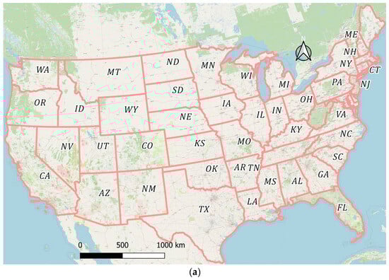
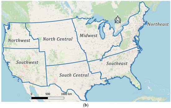
Figure 1.
The contiguous United States showing the main regional zones: (a) national extent; (b) division into seven principal hydrologic–administrative regions used in this study.
2.2. Data Compilation and Sources
A multi-source national dataset was compiled to describe flood events and their controlling physical and socioeconomic variables. The NOAA (www.noaa.gov) Storm Events Database served as the foundation of this study, documenting flood occurrences including event timing, location, and reported economic losses to property and agriculture [2,15]. To ensure a complete description of each event, the NOAA records were cross-referenced with complementary national datasets representing the hydrologic, climatic, topographic, and socioeconomic dimensions of flood behavior.
The National Water Model (NWM) (NOAA NWPS/NWM portal) provided physics-based, high-resolution hydrologic simulations based on the Weather Research and Forecasting–Hydrology WRF-Hydro framework, encompassing more than 8.1 million river reaches across the continental U.S. [20,21]. These data supply detailed streamflow and velocity estimates that capture the hydrologic dynamics of each flood event.
In addition to streamflow and velocity, the NWM provides a rich suite of hydrologic and land-surface variables essential for comprehensive flood modeling. Derived from its integrated land surface and routing components, the outputs include the following:
- Soil moisture and vertical variability: volumetric soil moisture is provided for multiple soil layers, along with soil saturation and ice fraction in the top 0.4 m.
- Evapotranspiration and evaporation processes: the model calculates accumulated total evapotranspiration (ACCET) as well as soil evaporation rates (EDIRs), enabling representation of water and energy fluxes in the water cycle.
- Infiltration dynamics: using the Green-Ampt-derived LGARTO soil infiltration scheme, NWM explicitly models vertical infiltration and runoff partitioning. In semiarid regions, it even accounts for channel infiltration, where water is lost from ephemeral streams into the subsurface [22].
- Water body evaporation and reservoir dynamics: the model simulates evaporation from lakes and reservoirs by tracking surface elevation, inflow/outflow, and ponded depth, integrating these into the overall water balance and energy exchange.
These detailed hydrologic processes, soil moisture dynamics, infiltration, evaporation, and reservoir routing are fully represented in our framework via direct ingestion of NWM outputs, ensuring a realistic simulation of key watershed and flood behaviors.
To represent storm magnitude and persistence, additional hydroclimatic indicators were derived from NOAA gridded precipitation and ground-station records. Event-based parameters included cumulative five-day rainfall, seven-day maximum precipitation, and five-day peak rainfall preceding each event. These indices describe both short-term storm severity and antecedent wetness conditions, key drivers of flood generation and intensity.
Topographic variables were obtained from the U.S. Geological Survey National Elevation Dataset (NED) (Download Data & Maps from The National Map|U.S. Geological Survey) [23,24]. This dataset, provided at a 100 m resolution under an Albers Equal-Area Conic projection, was used to derive catchment-scale metrics such as elevation, average slope, and distance to the nearest wadi (DTW). These parameters directly influence runoff concentration, flow routing, and inundation depth.
Flood exposure and vulnerability were represented through socioeconomic variables. Property values were extracted from the Zillow Home Value Index (ZHVI) (Housing Data—Zillow Research), which serves as a proxy for replacement cost and local economic conditions.
Population exposure was characterized using county-level data from the Surveillance, Epidemiology, and End Results (SEER) Program of the U.S. National Cancer Institute (NCI) (U.S. County Population Data 1969–2023—SEER Population Data), which provides annually updated population estimates consistent with U.S. Census standards [25].
2.3. Methodology
The proposed methodology (Figure 2) followed four integrated stages designed to ensure that flood damage costs were estimated consistently and transparently across the entire study area: Stage 1—Data integration and harmonization; Stage 2—Data analysis and feature preparation; Stage 3—Predictive model development and evaluation; and Stage 4—Framework deployment and validation.
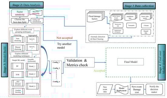
Figure 2.
Workflow of the nationwide flood-damage prediction framework showing the four sequential stages of data integration, analysis, model development, and validation.
2.3.1. Stage 1: Event Data Integration
Flood occurrences from the NOAA Storm Events Database were spatially and temporally aligned with the supporting datasets using a unified geospatial framework. Each flood record was linked with concurrent hydrologic, climatic, topographic, and socioeconomic attributes to ensure that both predictors and responses represented the same event in space and time rather than long-term averages.
2.3.2. Stage 2: Data Analysis and Pre-Processing
Rigorous data cleaning was conducted to remove duplicates and inconsistencies. Missing values were filled through interpolation or statistical imputation based on the type and correlation structure of the variables. Outliers were identified and corrected using the Interquartile Range (IQR) method, followed by validation through the Walsh test, which detects non-normal or median-deviant values via the Wilcoxon signed-rank statistics.
All numeric variables were normalized to a common scale to prevent domination by large-magnitude variables and enhance model stability. The final dataset was divided into training (70%), testing (15%), and validation (15%) subsets to ensure robust model calibration and independent performance assessment.
2.3.3. Stage 3: Predictive Model Development
Several predictive configurations were tested to determine the most reliable approach for nationwide damage-cost estimation. Each configuration was optimized and evaluated through the correlation coefficient (R) and bias (USD) metrics for training, testing, and validation datasets [2,26,27,28].
2.3.4. Stage 4: Framework Deployment and Validation
The final framework combined the classification and regression stages into a single, automated workflow (Figure 3). This structure handled normalization, oversampling, and feature selection, followed by parameter optimization to ensure repeatable and unbiased outcomes. The validated framework was then prepared for potential decision-support implementation, offering scalable capability for both real-time estimation and scenario-based flood-damage assessment. Continuous updates with new flood records will allow adaptive recalibration under evolving climatic and land-use conditions.
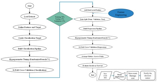
Figure 3.
Integrated classification–regression framework flow chart summarizing the full modeling pipeline.
3. Results
In the following sections, the results of the four methodology stages will be presented.
3.1. Stage 1: Data Preparation
To prepare training datasets that can be used for the training process, NOAA Storm Events Database was used to collect 17,407 flood occurrences between 1950 and 2022, including event timing, location, and reported economic losses to property and agriculture. Figure 4 shows NOAA 17,407 Flood events covering the full contiguous United States. Altogether, approximately 38 predictor variables were compiled across five main categories, climatic (NOAA), hydrologic (NWM), topographic (NED), geographic, and socioeconomic (ZHVI, SEER), as summarized in Table 1.
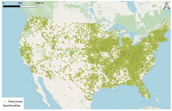
Figure 4.
NOAA 17,407 Flood events covering the full contiguous United States.

Table 1.
Factors influencing flood damage prediction.
3.1.1. Filling the Missing Data for the Median Home Prices Datasets
To address the study area’s lack of comprehensive temporal and geographical coverage of home price/value data, a variety of different machine learning models were examined to provide a more comprehensive benchmark and to determine whether different learning methodologies can enhance forecast accuracy to estimate median house prices at flood event sites and dates. The models included geographical and socioeconomic factors, including the following:
- Latitude and longitude are used to capture spatial heterogeneity in property values.
- Year and month are used to account for long-term trends and seasonal fluctuations in the housing market.
- Population represents population pressure and urban demand.
- County GeoID encodes administrative borders as well as the impacts of the area housing market.
The objective variable was the Zillow Home Value Index (ZHVI), which calculates median home values at the county level. The model was trained using historical ZHVI data and predictor factors taken from publicly available demographic and geographic information. A train-test split was used at the start of the modeling phase to guarantee a reliable assessment.
The final model’s performance using the Random Forest model was evaluated using bias and correlation coefficient metrics. The Random Forest model displayed good predictive performance, with a correlation coefficient of R = 0.95 between observed and anticipated values and a bias of −375 USD, indicating that it is suitable for reconstructing missing dwelling value data. Figure 5 depicts the Random Forest model’s comparison between the actual and predicted median house value. Now all collected datasets are completed and are ready for the next stage.
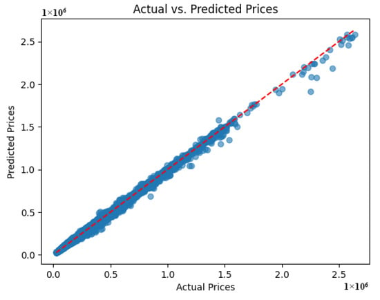
Figure 5.
The Random Forest model’s comparison between the actual and predicted median house values, with a correlation coefficient of R = 0.95 and a bias of −375 USD.
3.1.2. Exploring Machine Learning Algorithms
Eight different machine learning models were tested. Support Vector Regression (SVR) was used to capture nonlinear interactions with kernel-based techniques. A Multi-Layer Perceptron (MLP) Regressor, which represents a neural network technique, was used to assess the possibility of deep, nonlinear feature interactions. Gradient Boosting Regressor (GBR) was also evaluated as a boosting-based ensemble, allowing a direct comparison to RF’s bagging technique. Random Forest hyperparameters were adjusted using Randomized Search CV. Beyond these individual models, hybrid ensemble designs were investigated that coupled RF with other learners to capitalize on complementary abilities. These ensembles comprised RF coupled with Gradient Boosting, XGBoost, MLP, and Bayesian regression. This collection of models enabled us to thoroughly examine classical ensembles, neural network techniques, kernel-based learning, and hybrid ensemble tactics. Figure 6 shows the comparison using R testing and R training. Based on the results of the different machine learning models, the Random Forest model is the selected one, with a high value of R training and a corresponding high value of R testing.
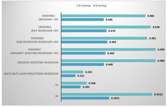
Figure 6.
The Random Forest model’s comparison with other selected models.
Random Forest (RF) was selected as the primary modeling approach due to several key advantages. It is highly robust to multicollinearity and noisy data, which are common characteristics of flood damage datasets. RF can effectively capture nonlinear relationships without requiring extensive parameter tuning, and its built-in feature importance ranking enhances interpretability in complex hydrological and socioeconomic contexts. Furthermore, RF offers scalability and computational efficiency for large datasets compared to kernel-based or deep learning models. Despite these strengths, RF has certain limitations, including reduced extrapolation capability beyond the training range and a tendency to bias toward dominant features. To mitigate these issues, hyperparameter tuning was performed using Randomized Search CV, improving model performance and reducing potential biases.
3.2. Stage 2: Data Analysis
3.2.1. Model Parameter Sensitivity and Feature Selection
A combination of automatic selection and manual testing was utilized to determine the optimal parameters and features for the finished flood damage prediction model. To determine which variables had the biggest impact on the model’s predictions, various feature groups were examined manually using the Random Forest (RF) feature importance results. In addition, an automated technique known as Recursive Feature Elimination with Cross-Validation (RFECV) was used to repeatedly validate the model and systematically eliminate less significant features. Combining human judgment with data-driven learning was made possible by using both strategies, resulting in a well-balanced model that operates accurately while maintaining its interpretability.
3.2.2. Predictive Features of Importance
An additional analysis examined the feature-importance rankings produced by the Random Forest model. As shown in Figure 7, variables such as latitude, longitude, elevation, and average catchment slope emerged as highly influential predictors. These reflect the combined influence of geographic setting, topographic controls, and short-term hydrologic intensity in shaping damage outcomes.
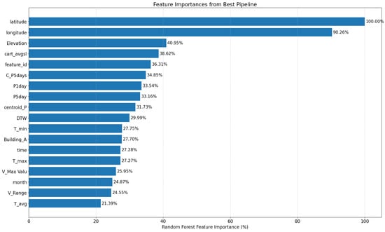
Figure 7.
Random Forest feature-importance rankings for the regression configuration, highlighting the key geographic and topographic drivers of damage.
3.2.3. Check Data Probability Distribution
Before conducting statistical analysis or predictive modeling, it is essential to examine the dataset’s probability distribution. This step ensures alignment with model assumptions and helps detect anomalies that could compromise accuracy. Visual tools such as histograms and kernel density plots offer an intuitive understanding of data shape and dispersion. In practice, data preparation often involves systematic preprocessing rather than relying solely on goodness-of-fit tests. In this study, the pipeline incorporates scaling (MinMaxScaler) to normalize feature ranges and resampling techniques like SMOTE to address class imbalance. These measures are particularly important for flood damage datasets, where catastrophic events frequently introduce skewness and heavy tails. Such treatments stabilize variance and enhance model performance, even when substantial discrepancies persist.
3.2.4. Anomaly Detection and Removal
Outliers, also known as anomalies, are data points that significantly deviate from expected patterns and can distort statistical metrics, leading to unreliable forecasts. In preparing flood damage datasets, identifying and correcting these anomalies is essential. In this study, outliers were detected and corrected using the Interquartile Range (IQR) method, which is effective for univariate analysis. To ensure robustness, the corrections were validated through the Walsh test, which identifies non-normal or median-deviant values using Wilcoxon signed-rank statistics. Incorporating domain knowledge remains critical extreme values may represent genuine catastrophic events rather than errors. Once anomalies are verified, strategies such as removal, capping, or imputation can be applied. Proper handling of anomalies ensures model reliability and forecasts that accurately reflect real flood damage scenarios.
3.3. Stage 3: Model Build
Four modeling configurations were implemented to estimate flood-damage costs across the contiguous United States, as summarized in Table 2. Each configuration represents a different strategy for combining climatic, geographic, temporal, hydrologic, topographic, and socioeconomic information into a predictive structure as follows:
Table 2.
Configuration Description.
- Configuration 1 (Manual Zoning): The contiguous United States was subdivided into predefined geographic zones for region-specific predictions.
- Configuration 2 (Automated Clustering): Data-driven grouping of similar events using K-Means, Agglomerative, and Gaussian Mixture Models [29,30,31,32,33,34].
- Configuration 3 (Direct Regression): Continuous prediction of damage costs using a Random Forest regression framework.
- Configuration 4 (Hybrid Classification and Regression): A two-step structure in which flood events were first categorized into risk levels (classification) and then refined by regression within each class [16].
All configurations were assessed using the correlation coefficient (R) and bias (USD) for training, testing, and validation datasets, enabling a fair comparison of their predictive skill and systematic error.
3.3.1. Configuration 1—Manual Zoning (Manual Clustering)
In the first configuration, the contiguous United States was manually divided into seven primary regional zones, Northwest, Southwest, Central North, Central South, Midwest, Northeast, and Southeast, to reflect broad contrasts in climate, hydrology, and socioeconomic conditions. Figure 1b shows the resulting regional partition used throughout the manual zoning experiments.
Within this framework, seven distinct zoning experiments (“trials”) were conducted to test different ways of grouping or merging these zones (Table 3). For each trial, separate sub-models were built within the specified zones, and model performance was evaluated using R and bias. This allowed the study to explore whether certain regional combinations better aligned with the underlying flood-damage patterns and to what extent manual zoning alone could enhance predictive skill. Figure 8 provides an overview of the manual zoning trials for the contiguous United States.
Table 3.
The 7 trials for manual zoning.
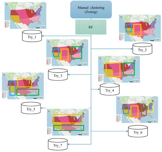
Figure 8.
Manual zoning trials for the contiguous United States illustrating the seven alternative regional combinations (as shown in Table 3).
We focused on seven representative clustering scenarios to keep the analysis practical and meaningful. Our approach was guided by three principles: first, clusters had to be made up of zones that share borders, so we avoided grouping regions that are geographically disconnected. Second, every trial needed to include all seven zones without overlaps or gaps, ensuring full coverage of the study area. Ultimately, we sought to identify clusters that highlight broad differences in climate, hydrology, and socioeconomic conditions across the contiguous United States. These contrasts matter because they influence flood risk and damage patterns. By applying these rules, we chose seven configurations that balance spatial logic with environmental and social diversity, giving us a clear and robust basis for comparison without introducing unnecessary complexity.
Among the seven trials, Trial 3 and Trial 6 yielded slightly higher correlation and lower bias than the others, suggesting that certain combinations of climatic zones better match the spatial structure of flood damage. However, as shown in Figure 9, the overall improvement across all trials remained modest. Manual zoning did not consistently deliver superior performance, and predictive accuracy was highly sensitive to how zones were merged. This highlights a key limitation of relying solely on expert-defined zones for a nationwide damage-prediction task: interpretability is high, but scalability and robustness are restricted.
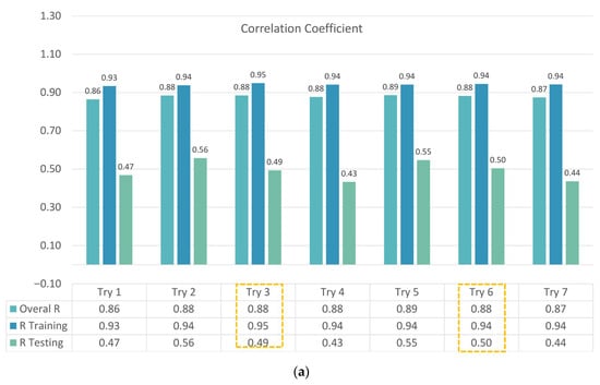
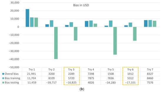
Figure 9.
(a) Correlation coefficient for the 7 trials covering training, testing, and overall performance. (b) Bias in USD for the 7 trials covering training, testing, and overall datasets. (The yellow boxes show the best trials).
3.3.2. Configuration 2—Automated Clustering
The second configuration replaced manual zoning with automated clustering, allowing the data itself to define groupings of flood events. This configuration is referred to as Config_2—Auto Clustering. To determine a suitable number of clusters, two standard diagnostic methods were used: (1) The Elbow method, which examines reductions in within-cluster variance as the number of clusters increases; (2) The Silhouette method, which evaluates how well each event fits within its assigned cluster compared to neighboring clusters. As shown in Figure 10, the elbow curve indicated a point of diminishing returns, and the Silhouette analysis identified four clusters as the most meaningful representation of event distribution.
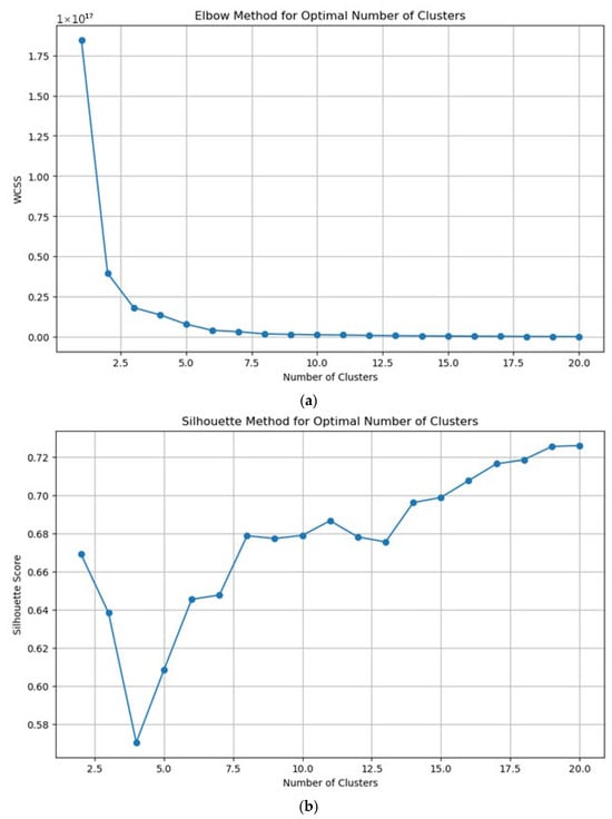
Figure 10.
Diagnostic plots are used to select the number of clusters: (a) Elbow method; (b) Silhouette method, highlighting four clusters as the most suitable solution.
Three alternative clustering algorithms were then tested: K-Means, Agglomerative, and Gaussian Mixture Model (GMM) (refer to Appendix A, Figure A1, and Table A1 for full cluster results). Each algorithm produced a four-cluster solution, but with different internal structures and degrees of overlap. Their predictive performance was compared using R and bias for both training and testing datasets.
Figure 11 summarizes these comparisons. While all three techniques displayed similar patterns, K-Means consistently achieved slightly higher correlation and lower bias across the four-cluster solution. This balance of simplicity and performance made K-Means the most practical clustering option for subsequent modeling.
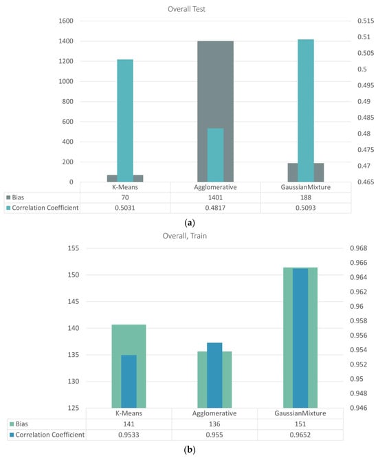
Figure 11.
(a) Overall, four cluster testing results for the correlation coefficient (right axis) and bias in USD (left axis). (b) Overall, four cluster training results for the correlation coefficient (right axis) and bias in USD (left axis).
Overall, the automated clustering configuration improved upon manual zoning by providing data-driven groupings that better capture the structure of flood-damage variability, with less dependence on subjective regional boundaries. However, the performance of R values remains low, especially for the testing data, indicating that further improvements to this configuration are still needed. Additionally, a new evaluation approach should be introduced to enhance performance in terms of both R values and bias.
3.3.3. Configuration 3—Direct Regression (Approach 1)
The third configuration (Config_3—Approach 1: Regression) applied regression models directly to the full dataset without prior zoning or clustering. Here, the objective was to relate flood-damage costs to the full set of predictor variables and evaluate how well a purely regression-based approach could generalize.
A comprehensive sensitivity analysis was performed to identify the most influential factors and reduce redundancy. Out of the initial 38 variables, a reduced subset of 18 predictors was found to yield more stable and consistent results. Several regression models were compared, with Random Forest regression providing the best overall predictive performance.
Figure 12 presents the Random Forest correlation coefficients and biases for the training, testing, and overall datasets. The model demonstrated strong agreement between predicted and observed damages, with improved correlation and reduced bias compared to the clustering-based setups. However, verification using testing data revealed limitations: the testing correlation reached R = 0.60, and the bias testing values touched approximately −480 USD. These results indicate that while the regression-based approach improved internal consistency, its generalization capability was insufficient, motivating the need to explore the final configuration for better robustness.
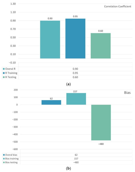
Figure 12.
Random Forest regression performance in Configuration 3: (a) correlation coefficients for training, testing, and overall datasets; (b) corresponding bias in USD.
3.3.4. Configuration 4—Hybrid Classification + Regression (Approach 2)
At the beginning of this configuration, it is noted to mention that one new engineering feature was added to the parameters, which is called parameter. A composite indicator, Price − Risk, was created to capture both exposure and hazard intensity using
where the Risk Level was derived from preliminary classification of damage cost categories using Random Forest classification (Figure 13).
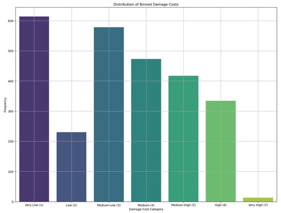
Figure 13.
Example of the seven damage categories used for model classification in the Random Forest stage: Damage costs were discretized into seven categories These categories represent increasing ranges of damage cost: Category 1 (≤1000), Category 2 (1001–2000), Category 3 (2001–5000), Category 4 (5001–12,000), Category 5 (12,001–25,000), Category 6 (25,001–59,000), and Category 7 (>59,000).
The fourth configuration (Config_4—Approach 2) adopted a hybrid two-step structure, in which
- (1)
- A classification stage assigned each flood event to one of seven ordered risk categories based on damage cost;
- (2)
- A regression stage then estimated continuous damage values within each category.
Classification Process
In the first phase, a Random Forest classifier analyzed the full set of available parameters to predict the risk level of each flood event. The model used seven ordered damage groups (Figure 13) and incorporated a processed pipeline that included: Missing-value imputation, Min–Max scaling, and Synthetic Minority Oversampling (SMOTE) to address class imbalance, with hyperparameters tuned via Randomized Search CV. Performance was evaluated using a 40-fold K-Fold procedure, generating confusion matrices and classification reports for each fold.
Figure 14 displays a representative confusion matrix and classification report. These outputs illustrate that the model distinguishes risk categories reliably, with particularly strong performance for the highest-damage classes and expected overlap between mid-level categories due to the continuous nature of loss values (Appendix B Figure A2 shows all the fold classes’ classification results).
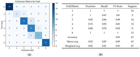
Figure 14.
Sample Random Forest classifier results for one-fold: (a) confusion matrix; (b) classification report summarizing accuracy and precision across damage categories.
This phase not only provides a clear categorical description of damage severity but also enables the construction of engineered variables such as the Price_Risk component, which blends property values and risk level to support downstream regression.
Regression Process
The second phase focused on predicting continuous damage costs using Random Forest regression, applied within the pre-defined risk categories. The regression pipeline included preprocessing, feature scaling, hyperparameter optimization (Randomized Search CV), and feature selection through RFECV. Again, a 40-fold K-Fold procedure was used to evaluate accuracy and stability.
Fold-by-fold feature-importance plots consistently identified Price_Risk, geographic coordinates, and population as key drivers. Figure 15 summarizes (a) the average feature-importance ranking across folds, as well as (b) the density plot comparing predicted versus actual damage costs.
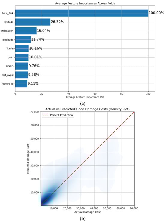
Figure 15.
Hybrid regression performance in Configuration 4: (a) average Random Forest regressor feature importance across folds; (b) density plot of actual vs. predicted flood-damage costs.
When evaluated on an independent validation dataset, the hybrid configuration achieved R ≈ 0.811 on the validation set, and an average bias of about −275 USD, indicating strong agreement with observed damages and only a very small systematic underestimation relative to the magnitude of total losses. The following illustration (Figure 16) highlights these findings by displaying a side-by-side comparison of the correlation coefficient and bias as a column chart, emphasizing the model’s strong performance and low systematic error.
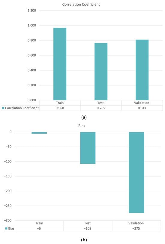
Figure 16.
(a) Model correlation coefficient for the training, testing, and validation data sets. (b) Model Bias for the training, testing, and validation data sets.
3.3.5. Comparative Evaluation Across Configurations
To synthesize results, the performance of the best model from all four configurations was compared using R and bias for testing data. Figure 17 presents a side-by-side column-chart comparison of correlation and bias across the configurations.
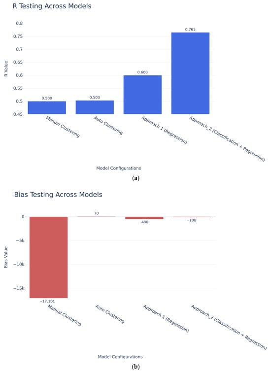
Figure 17.
Comparison of model performance across configurations: (a) correlation coefficients for testing datasets; (b) corresponding testing bias (USD) for each configuration.
Key observations are as follows. Manual zoning (Config_1) provided useful regional insight but showed limited improvement even after multiple trials. Automated clustering (Config_2) produced more coherent groups and modest performance gains. Direct regression (Config_3) yielded stronger and more interpretable relationships, especially after reducing the predictor set to 18 variables. The hybrid classification–regression configuration (Config_4) delivered the best overall performance, combining high correlation with low bias and stable results across datasets. These findings support the adoption of the hybrid framework as the recommended operational structure for nationwide flood-damage estimation.
3.4. Stage 4: Final User Model
This stage brings together two complementary processes classification and regression within an integrated modeling framework (Figure 3). The classification component provides clear and interpretable categories of flood risk levels, while the regression phase refines these outcomes into accurate predictions of economic damage costs. Both steps operate through well-structured pipelines that handle data imputation, normalization, oversampling, and model tuning using RandomizedSearchCV, ensuring reliable and repeatable results. The overall workflow starts with data preparation and moves through risk level classification, engineered feature creation, recursive feature selection, and regression evaluation, ending with a comprehensive performance assessment.
Finally, the best-performing model is finalized using the refined flood dataset after removing anomalies and verifying input consistency. Once validated, the model is deployed as part of a decision-support framework for real-time flood damage estimation, enabling timely and informed responses. To maintain its accuracy and relevance over time, the model is periodically updated and recalibrated with new flood event data, ensuring long-term reliability and adaptability in changing environmental conditions.
4. Discussion
The nationwide, event-based modeling framework developed in this study successfully estimated flood-damage costs across the contiguous United States by integrating hydrologic, climatic, topographic, and socioeconomic datasets.
Among the four tested configurations manual zoning, automated clustering, direct regression, and hybrid classification/regression, the hybrid configuration (Config 4) achieved the best overall performance (R = 0.81, bias = −274.5 USD on validation), as shown in Figure 16. The hybrid model consistently produced higher correlation coefficients and lower biases than all other configurations, confirming the advantage of a two-stage design that first classifies flood events into risk levels and then refines continuous loss estimates within each class. This structure improved predictive stability and interpretability, particularly for high-damage, low-frequency events that traditionally challenge large-scale flood-damage models. The hybrid configuration outperformed all other tested approaches in both accuracy and robustness.
The automated clustering method improved model generalization over manual zoning by allowing data-driven regionalization (see Figure 11), while the direct regression approach (Figure 12) provided improved predictive strength by optimizing variable selection. However, the hybrid model combined the advantages of both, achieving higher consistency across all datasets (training, testing, and validation).
Feature-importance analysis (Figure 15a) revealed that median home value (ZHVI), maximum 5-day rainfall, population density, and streamflow were the most influential predictors. These jointly explained about 70% of the observed variance, confirming that flood losses are governed by both hazard intensity and exposure, rather than by hydrologic conditions alone.
Overall, the hybrid configuration maintained near-zero bias across the national domain, confirming its ability to generalize effectively despite regional differences in data density or flood typology. The hybrid framework provides both technical and practical value for large-scale flood-loss estimation.
At the technical level, it demonstrates that integrating hydrologic and socioeconomic data through ensemble learning can produce reliable, transferable models. At the practical level, it can serve as a decision-support tool for the following: (1) Rapid assessment of potential flood losses by emergency and insurance agencies; (2) Strategic identification of high-risk zones for infrastructure investment; (3) Policy formulation for national flood-risk reduction and adaptation strategies.
The proportions of variable contributions are 45% socioeconomic, 40% hydrologic–climatic, and 15% topographic/geographic, which also reinforce the importance of combining physical and exposure factors to understanding flood impacts [2,8,15,16].
Imputing socioeconomic variables, particularly property values, can introduce uncertainty that may propagate into flood damage estimates. This issue is widely recognized in the literature. For example, Khalil et al. (2006) emphasized that explicitly accounting for uncertainty in model structure and data availability improves prediction reliability [4], while Wagenaar et al. (2017) and Schröter et al. (2014) noted that gaps in socioeconomic data can significantly affect damage estimation accuracy [1,6]. Similar approaches have been used in other flood damage prediction studies, such as. Alipour et al. (2020), which complemented missing house price data through structured imputation to improve model completeness in a Southeast region study [2]. In our study, imputation was necessary to harmonize a multi-source national database and ensure model completeness. To minimize potential bias, structured imputation techniques were applied using a regional Random Forest model and historical property records rather than simplistic assumptions. Model performance was further evaluated across multiple zoning configurations to detect systematic errors. Despite these measures, residual uncertainty remains, particularly in regions with scarce socioeconomic data. Future research could explore probabilistic imputation strategies or incorporate uncertainty quantification frameworks as potential ways to better capture and communicate these uncertainties in house cost estimation.
To complement the performance evaluation, we conducted interpretability analyses to better understand the physical and hydrological drivers of flood damage. These analyses aim to bridge the gap between predictive accuracy and process-based reasoning, providing insights into how key variables influence damage outcomes.
SHAP (SHapley Additive exPlanations)-based feature importance analysis provides insights into the hydrological and physical processes influencing flood damage, as demonstrated by Li, Z. et al. (2025) [35]. Geographic location (latitude, longitude) dominates the model, reflecting spatial variability in exposure and vulnerability. Among hydrological and climatic factors, cumulative precipitation (centroid_P, P7day, P5day) and maximum flow velocity (V_Max Value) emerge as influential, suggesting that both antecedent wetness and flow dynamics contribute significantly to damage outcomes. SHAP leverages cooperative game theory to fairly attribute each feature’s contribution to predictions, considering all possible feature interactions. This approach not only ranks features by importance but also explains the direction and magnitude of their influence, making complex models more transparent and interpretable for decision-making.
Topographic variables such as elevation and catchment area also rank highly, consistent with their role in runoff concentration and inundation depth. These findings align with hydrological theory and indicate that damage patterns may differ across flood typologies (e.g., flash floods versus riverine floods). While this study does not perform a full typology-based analysis, these results underscore the need for future research integrating physical process modeling with damage prediction.
Additional interpretability analyses, including a correlation matrix between the predictor and SHAP-based feature importance, are provided in Appendix C, Figure A3 and Figure A4.
4.1. Benchmarking Against Previous Studies
There are several differences between our findings and those of previous research. The benefits of incorporating a more comprehensive set of geospatial, hydrological, and socioeconomic factors over a wider spatial domain were highlighted by a study that was restricted to the flash flood in Figure 18 of the Southeast United States and revealed poorer predictive accuracy, lower correlation coefficients, and a more noticeable bias than our model [2].
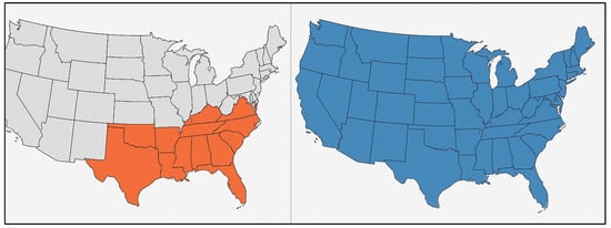
Figure 18.
The previous study focused solely on the Southeast region (at left), flash flood-only, achieving R = 0.71 (testing) and R = 0.90 (training). The model showed a negative bias, with mean errors of −$1100 in testing and −$1010 overall.
Another nationwide study, on the other hand, used a two-step framework of damage level classification followed by claim number regression, with subsampling procedures to mitigate overfitting and underfitting caused by the skewed distribution of claims. This study modeled expected flood insurance claims rather than monetary losses [16]. Although this framework takes a novel approach, it is nevertheless limited by its emphasis on claim numbers rather than the precise cost of damage. Furthermore, our study already integrates a more additional factors directly into a cost-based prediction framework, notwithstanding the authors’ valid suggestions to relate socioeconomic and demographic data to flood risk and to expand historical records to investigate climatic variability. Furthermore, a more recent statewide research effort has created the first spatially comprehensive map of flood damage likelihood; however, it was limited to categorizing whether damage would occur rather than determining actual costs [19]. Consistency was limited by the claimed accuracy by type of land cover. By explicitly measuring monetary damages, our study goes beyond probability mapping and provides more useful outputs for resource allocation and planning.
By integrating physical and socioeconomic predictors within a unified, data-driven system, the framework achieved high predictive accuracy (R = 0.81) with minimal bias (−274.5 USD), outperforming earlier nationwide efforts such as those by Schröter et al. (2014) [6], Yang et al. (2022) [16], and Collins et al. (2022) [19].
4.2. Modeling Approaches for Flood Damage Prediction: Strengths, Limits, and Future Directions
Different modeling approaches each have their own strengths and limitations for predicting flood damage. Random Forest (RF) is particularly attractive because it handles multicollinearity and noisy data well and can capture complex nonlinear relationships without requiring extensive parameter tuning. Its built-in feature importance measures also help with interpretability, which is especially valuable in socioeconomic and hydrological applications. However, RF does not extrapolate well beyond the range of the training data and can be biased toward features that dominate the dataset.
Quantile-based methods were not used in this study, but they represent a promising direction for future work, especially for improving how we quantify uncertainty in flood damage predictions. Instead of estimating only the mean outcome, these approaches model conditional quantiles, making them useful for understanding uncertainty and extreme events. They are generally easy to interpret and well-suited for risk assessment, although they may struggle with highly nonlinear interactions unless combined with more flexible modeling techniques.
Deep learning models are powerful tools for capturing complex patterns in large, high-dimensional datasets and often achieve higher predictive accuracy than more traditional methods. However, they require large amounts of data and substantial computational resources. Their “black-box” nature also makes them difficult to interpret, which is a major drawback in policy-oriented flood risk management.
Probabilistic methods, such as Bayesian approaches, offer a principled way to quantify uncertainty and incorporate prior knowledge into the modeling process. These methods are particularly valuable for decision-making under uncertainty. Nonetheless, they can be computationally demanding and may not scale easily to very large datasets, such as extensive records of flood damage events.
Finally, it is important to note that Random Forest has also been used successfully beyond damage estimation. Soliman et al. (2025) developed a generalized ML-based approach to predict two-dimensional flood depths using freely available global datasets and a large set of diverse catchments [36]. After comparing several algorithms, they selected Random Forest for both flood inundation mapping and flood depth prediction, achieving high validation while producing complete flood depth maps in more than two orders of magnitude faster than traditional hydraulic simulations. These findings support the idea that Random Forest can act as a practical, scalable backbone for flood modeling, which is consistent with its role in the present study. Looking ahead, future machine learning frameworks will likely combine the strengths of RF, quantile-based methods, deep learning, and probabilistic approaches, leading to more comprehensive and robust models for event-based flood damage prediction
5. Conclusions
This study presents the first nationwide, event-based hybrid modeling framework for flood-damage cost prediction across the contiguous United States. The key outcomes can be summarized as follows:
- Integration of multi-source datasets hydrologic (NWM), climatic (NOAA), topographic (NED), and socioeconomic (ZHVI, SEER) enabled event-specific, physically consistent predictions.
- Hybrid two-stage design (classification followed by regression) enhanced accuracy, interpretability, and robustness, especially for rare, high-damage events.
- Socioeconomic exposure and vulnerability proved as influential as hydrologic drivers, confirming the interdependence of hazard and exposure in national flood losses.
- The model’s scalable, automated workflow can be updated as new flood records become available, supporting its evolution into a real-time or near-real-time operational platform.
The novelty of this study lies in its ability to predict actual monetary flood damage costs at the event scale, rather than probabilities or claims counts, making results more actionable for planning and resource allocation. It combines climatic, hydrologic, topographic, and socioeconomic predictors across the entire U.S., introduces 25 new variables, and rigorously evaluates eight machine learning models to ensure robustness. The framework achieves high accuracy and low bias, outperforming previous regional efforts and demonstrating scalability for nationwide application.
Future work should focus on expanding data coverage and incorporating remote-sensing flood-inundation data and real-time hydrometeorological inputs to improve spatial and temporal precision. The approach can also be adapted for other regions globally, providing a transferable template for national-scale flood-loss modeling.
Overall, this framework represents a significant step toward data-driven, operational flood-damage cost prediction, offering a scientifically robust basis for managing and mitigating flood risk across the United States.
Author Contributions
Conceptualization, M.M.M. and H.G.R.; methodology, K.M.A., M.M.M. and H.G.R.; software, K.M.A. and M.M.M.; validation, K.M.A. and M.M.M.; formal analysis, M.M.M. and H.G.R.; data curation, M.M.M. and H.G.R.; writing—original draft preparation, K.M.A. and M.M.M.; writing—review and editing, M.M.M. and H.G.R.; visualization, M.M.M. and H.G.R.; supervision, M.M.M. and H.G.R. All authors have read and agreed to the published version of the manuscript.
Funding
This research received no external funding.
Data Availability Statement
Data used in this research are available online as follows: NOAA Storm Events Database is available at https://www.noaa.gov (accessed on 30 June 2021). National Water Model (NWM) is available at https://water.noaa.gov (accessed on 30 November 2023). U.S. Geological Survey National Elevation Dataset (NED) is available at https://www.usgs.gov/national-map (accessed on 1 October 2012). Zillow Home Value Index (ZHVI) is available at https://www.zillow.com/research/data (accessed on 7 December 2024). SEER County Population Data is available at https://seer.cancer.gov/popdata (accessed on 11 December 2024). Additional hydroclimatic indicators were derived from NOAA gridded precipitation and ground-station records, accessed on 30 June 2021 via NOAA’s data portals.
Conflicts of Interest
The authors declare no conflict of interest.
Abbreviations
The following abbreviations are used in this manuscript:
| ACCET | Accumulated Total Evapotranspiration |
| EDIR | Direct Soil Evaporation Rate |
| LGARTO | Layered Green-Ampt with Redistribution and Optimization |
| NCI | National Cancer Institute |
| NED | National Elevation Dataset. |
| NOAA | The National Oceanic and Atmospheric Administration. |
| SEER | US National Cancer Institute’s Surveillance, Epidemiology, and End Results. |
| SHAP | SHapley Additive exPlanations |
| USGS | United States Geological Survey |
| WRF-Hydro | Weather Research and Forecasting–Hydrology |
| ZHVI | Zillow Home Value Index |
Appendix A. Clustering Methods Visualization
To further highlight the clustering process, three methods, K-Means, Agglomerative, and Gaussian Mixture Models, were used, and their results were shown (Table A1) using three-dimensional Principal Component Analysis. The 3D PCA plots (Figure A1) give an intuitive perspective of how flood events are distributed among clusters for each approach, allowing for visual examination of separation quality and overlap. While dimensionality reduction cannot capture all variability in the data, it can offer a clear comparison view of cluster borders and event groupings.
Furthermore, the number of flood events allocated to each cluster was summed and shown as column charts (Figure A1). These plots indicate the balance (or imbalance) of event distribution among clusters for each approach, such as how some methods created one huge dominant cluster with lesser ones, while others produced more balanced partitions. The PCA scatter plots and column charts work together to offer a geometric and numerical comprehension of the clustering findings, supplementing the statistical analysis presented in the main results.


Figure A1.
Different Clustering methods, distribution, and PCA Visualization: (a) K-Means; (b) Agglomerative; (c) Gaussian Mixture.
Table A1.
Different Clustering methods internal cluster outcomes for bias and correlation coefficient, showing the testing and training data sets results.
Table A1.
Different Clustering methods internal cluster outcomes for bias and correlation coefficient, showing the testing and training data sets results.
| Method | cluster_0 | cluster_1 | cluster_2 | cluster_3 | ||||||||||||
|---|---|---|---|---|---|---|---|---|---|---|---|---|---|---|---|---|
| R | Bias | R | Bias | R | Bias | R | Bias | |||||||||
| Test | Train | Test | Train | Test | Train | Test | Train | Test | Train | Test | Train | Test | Train | Test | Train | |
| K-Means | 0.369 | 0.944 | 921 | 183 | 0.509 | 0.954 | 431 | 129 | 0.619 | 0.959 | −179 | 123 | 0.516 | 0.956 | −892 | 125 |
| Agglomerative | 0.406 | 0.952 | 480 | 122 | 0.592 | 0.955 | 461 | 138 | 0.365 | 0.955 | 362 | 121 | 0.563 | 0.957 | 4298 | 159 |
| Gaussian Mixture | 0.446 | 0.973 | 528 | 196 | 0.633 | 0.980 | −747 | 126 | 0.452 | 0.952 | 1048 | 173 | 0.506 | 0.956 | −77 | 109 |
Appendix B. Classification Model Results


Figure A2.
Confusion matrix for each fold in the classification part of the model.
Appendix C. Additional Interpretability Analyses

Figure A3.
The correlation matrix shows interrelations among predictors.

Figure A4.
SHAP-based feature importance.
References
- Wagenaar, D.; de Jong, J.; Bouwer, L.M. Multi-variable flood damage modelling with limited data using supervised learning approaches. Nat. Hazards Earth Syst. Sci. 2017, 17, 1683–1696. [Google Scholar] [CrossRef]
- Alipour, A.; Ahmadalipour, A.; Abbaszadeh, P.; Moradkhani, H. Leveraging machine learning for predicting flash flood damage in the Southeast US. Environ. Res. Lett. 2020, 15, 024011. [Google Scholar] [CrossRef]
- El-Jabi, N.; Rousselle, J. A Flood Damage Model for Flood Plain Studies. J. Am. Water Resour. Assoc. 1987, 23, 179–187. [Google Scholar] [CrossRef]
- Khalil, A.F.; McKee, M.; Kemblowski, M.; Asefa, T.; Bastidas, L. Multiobjective analysis of chaotic dynamic systems with sparse learning machines. Adv. Water Resour. 2006, 29, 72–88. [Google Scholar] [CrossRef]
- Ten Veldhuis, J.A.E. How the choice of flood damage metrics influences urban flood risk assessment. J. Flood Risk Manag. 2011, 4, 281–287. [Google Scholar] [CrossRef]
- Schröter, K.; Kreibich, H.; Vogel, K.; Riggelsen, C.; Scherbaum, F.; Merz, B. How useful are complex flood damage models? Water Resour. Res. 2014, 50, 3378–3395. [Google Scholar] [CrossRef]
- Sieg, T.; Vogel, K.; Merz, B.; Kreibich, H. Tree-based flood damage modeling of companies: Damage processes and model performance. Water Resour. Res. 2017, 53, 6050–6068. [Google Scholar] [CrossRef]
- Wagenaar, D.; Lüdtke, S.; Schröter, K.; Bouwer, L.M.; Kreibich, H. Regional and Temporal Transferability of Multivariable Flood Damage Models. Water Resour. Res. 2018, 54, 3688–3703. [Google Scholar] [CrossRef]
- Gutenson, J.L.; Ernest, A.N.S.; Oubeidillah, A.A.; Zhu, L.; Zhang, X.; Sadeghi, S.T. Rapid Flood Damage Prediction and Forecasting Using Public Domain Cadastral and Address Point Data with Fuzzy Logic Algorithms. J. Am. Water Resour. Assoc. 2018, 54, 104–123. [Google Scholar] [CrossRef]
- Ozger, M. Assessment of flood damage behaviour in connection with large-scale climate indices. J. Flood Risk Manag. 2017, 10, 79–86. [Google Scholar] [CrossRef]
- Vogel, K.; Weise, L.; Schröter, K.; Thieken, A.H. Identifying Driving Factors in Flood-Damaging Processes Using Graphical Models. Water Resour. Res. 2018, 54, 8864–8889. [Google Scholar] [CrossRef]
- Snehil; Goel, R. Flood Damage Analysis Using Machine Learning Techniques. Procedia Comput. Sci. 2020, 173, 78–85. [Google Scholar] [CrossRef]
- Lee, K.; Choi, C.; Shin, D.H.; Kim, H.S. Prediction of heavy rain damage using deep learning. Water 2020, 12, 1942. [Google Scholar] [CrossRef]
- Shaharkar, A.; Sonar, Y.; Sonar, A.; Pawar, C. Flood Damage Estimation using Machine Learning in GIS. Int. Res. J. Eng. Technol. 2020, 7, 5756–5760. [Google Scholar]
- Alipour, A.; Ahmadalipour, A.; Moradkhani, H. Assessing flash flood hazard and damages in the southeast United States. J. Flood Risk Manag. 2020, 13, e12605. [Google Scholar] [CrossRef]
- Yang, Q.; Shen, X.; Yang, F.; Anagnostou, E.N.; He, K.; Mo, C.; Seyyedi, H.; Kettner, A.J.; Zhang, Q. Predicting Flood Property Insurance Claims over CONUS, Fusing Big Earth Observation Data. Bull. Am. Meteorol. Soc. 2022, 103, E791–E809. [Google Scholar] [CrossRef]
- Harris, R.; Furlan, E.; Pham, H.V.; Torresan, S.; Mysiak, J.; Critto, A. A Bayesian network approach for multi-sectoral flood damage assessment and multi-scenario analysis. Clim. Risk Manag. 2022, 35, 100410. [Google Scholar] [CrossRef]
- Parvin, F.; Ali, S.A.; Calka, B.; Bielecka, E.; Linh, N.T.T.; Pham, Q.B. Urban flood vulnerability assessment in a densely urbanized city using multi-factor analysis and machine learning algorithms. Theor. Appl. Climatol. 2022, 149, 639–659. [Google Scholar] [CrossRef]
- Collins, E.L.; Sanchez, G.M.; Terando, A.; Stillwell, C.C.; Mitasova, H.; Sebastian, A.; Meentemeyer, R.K. Predicting Flood Damage Probability across the Conterminous United States. Environ. Res. Lett. 2022, 17, 034006. [Google Scholar] [CrossRef]
- Johnson, J.M.; Munasinghe, D.; Munasinghe, M.; Cohen, S. Evaluating the National Water Model’s Height Above Nearest Drainage (HAND) Flood Mapping Methodology Across the Continental United States. Nat. Hazards Earth Syst. Sci. 2019, 19, 2405–2420. [Google Scholar] [CrossRef]
- Wang, Y.; Shen, H.; Xu, H. A Data-Driven Framework for Flood Inundation Forecasting Using the National Water Model and VIIRS Observations. Remote Sens. 2024, 16, 4357. [Google Scholar] [CrossRef]
- Lahmers, T.M.; Hazenberg, P.; Gupta, H.; Castro, C.; Gochis, D.; Dugger, A.; Yates, D.; Read, L.; Karsten, L.; Wang, Y.-H. Evaluation of NOAA National Water Model Parameter Calibration in Semiarid Environments Prone to Channel Infiltration. J. Hydrometeorol. 2021, 22, 2939–2969. [Google Scholar] [CrossRef]
- Gesch, D.B.; Oimoen, M.J.; Nelson, G.A.; Steuck, M.; Tyler, D. The National Elevation Dataset. Photogramm. Eng. Remote Sens. 2002, 68, 5–11. [Google Scholar]
- Gesch, D.B.; Oimoen, M.J.; Evans, G.A. Accuracy Assessment of the U.S. Geological Survey National Elevation Dataset, and Comparison with Other Large-Area Elevation Datasets—SRTM and ASTER. USGS Open-File Rep. 2014, 2014, 10. [Google Scholar] [CrossRef]
- National Cancer Institute; National Center for Health Statistics; U.S. Census Bureau. U.S. Population Data SEER Program. Surveillance, Epidemiology, and End Results (SEER) Program. 2025. Available online: https://seer.cancer.gov/data-software/uspopulations.html (accessed on 11 December 2024).
- Shastry, A.; Durand, M. Utilizing Flood Inundation Observations to Obtain Floodplain Topography in Data-Scarce Regions. Front. Earth Sci. 2019, 6, 243. [Google Scholar] [CrossRef]
- Abbaszadeh, P.; Moradkhani, H.; Daescu, D.N. The Quest for Model Uncertainty Quantification: A Hybrid Ensemble and Variational Data Assimilation Framework. Water Resour. Res. 2019, 55, 2407–2431. [Google Scholar] [CrossRef]
- Neri, A.; Villarini, G.; Salvi, K.A.; Slater, L.J.; Napolitano, F. On the Decadal Predictability of the Frequency of Flood Events across the U.S. Midwest. Int. J. Climatol. 2019, 39, 1796–1804. [Google Scholar] [CrossRef]
- Kaufman, L.; Rousseeuw, P.J. Finding Groups in Data: An Introduction to Cluster Analysis; John Wiley & Sons: New York, NY, USA, 1990. [Google Scholar] [CrossRef]
- Rousseeuw, P.J. Silhouettes: A Graphical Aid to the Interpretation and Validation of Cluster Analysis. J. Comput. Appl. Math. 1987, 20, 53–65. [Google Scholar] [CrossRef]
- Sugar, C.A.; James, G.M. Finding the Number of Clusters in a Dataset: An Information-Theoretic Approach. J. Am. Stat. Assoc. 2003, 98, 750–763. [Google Scholar] [CrossRef]
- MacQueen, J.B. Some Methods for Classification and Analysis of Multivariate Observations. In Proceedings of the Fifth Berkeley Symposium on Mathematical Statistics and Probability, Berkeley, CA, USA, 21 June–18 July 1965, 27 December 1965–7 January 1966; University of California Press: Berkeley, CA, USA, 1965; Volume 1, pp. 281–297. [Google Scholar]
- McLachlan, G.; Peel, D. Finite Mixture Models; Wiley Series in Probability and Statistics; John Wiley & Sons: New York, NY, USA, 2000. [Google Scholar] [CrossRef]
- Ward, J.H. Hierarchical Grouping to Optimize an Objective Function. J. Am. Stat. Assoc. 1963, 58, 236–244. [Google Scholar] [CrossRef]
- Li, Z.; Tian, J.; Zhu, Y.; Chen, D.; Ji, Q.; Sun, D. A Study on Flood Susceptibility Mapping in the Poyang Lake Basin Based on Machine Learning Model Comparison and SHapley Additive exPlanations Interpretation. Water 2025, 17, 2955. [Google Scholar] [CrossRef]
- Soliman, M.; Morsy, M.M.; Radwan, H.G. Generalized Methodology for Two-Dimensional Flood Depth Prediction Using ML-Based Models. Hydrology 2025, 12, 223. [Google Scholar] [CrossRef]
Disclaimer/Publisher’s Note: The statements, opinions and data contained in all publications are solely those of the individual author(s) and contributor(s) and not of MDPI and/or the editor(s). MDPI and/or the editor(s) disclaim responsibility for any injury to people or property resulting from any ideas, methods, instructions or products referred to in the content. |
© 2026 by the authors. Licensee MDPI, Basel, Switzerland. This article is an open access article distributed under the terms and conditions of the Creative Commons Attribution (CC BY) license.