Experimental Study of Hydrodynamics During Fluid Flow from a Nozzle in a Differential-Contact Centrifugal Extractor

Abstract

Modern processes to produce rare-earth elements, strategic metals, and nuclear fuel reprocessing require highly efficient liquid–liquid extraction in systems characterized by high viscosity, elevated interfacial tension, and small density differences. Traditional gravity-driven extractors exhibit low performance under these conditions, whereas centrifugal extractors enable rapid mass transfer and nearly complete phase separation. Differential-contact annular centrifugal contactors offer the highest flexibility and efficiency, but their optimization is limited by the lack of experimental data on the hydrodynamics of liquid flow through perforated nozzles in a rotating field. This limitation hinders the development of accurate computational fluid dynamics (CFD) models (e.g., ANSYS Fluent), reliable equipment scale-up, and the design of optimized contactor configurations. The present study addresses this gap by experimentally determining the flow velocity of liquids through nozzles of various geometries across a wide range of centrifugal accelerations. From these data, a universal power-law correlation was derived, linking the flow rate to rotor speed, nozzle geometry, and the physicochemical properties of the phases. The proposed correlation provides a robust experimental basis for numerical model validation, computational design, and optimization of next-generation differential-contact centrifugal extractors.

1. Introduction

Modern chemical and technological processes for recovering rare earth elements, strategic metals, reprocessing nuclear fuel, and purifying high-activity waste increasingly demand highly efficient liquid–liquid extraction methods [1,2,3]. These systems are often characterized by small differences in phase densities ($\rho$), high interfacial tension ($\sigma$), and increased viscosity ($\mu$) of organic extractants [4]. Under such challenging conditions, traditional gravity-driven devices, such as columns and mixer-settlers, often exhibit low productivity and require large physical footprints [5]. Conversely, centrifugal extractors enable intensive mass transfer and nearly complete phase separation in seconds rather than minutes [6]. This performance advantage has been extensively documented in recent studies, including works on extraction efficiency and phase separation kinetics [7].

Among the various centrifugal designs, differential-contact devices—specifically Annular Centrifugal Contactors (ACC) and classic Podbielniak-type machines—have demonstrated significant versatility [8]. Their operation relies on the multiple dispersion of one phase into another through perforated cylindrical nozzles (dispersers), followed by rapid coalescence induced by a strong centrifugal field [9]. The presence of multiple contact zones, formed by coaxial perforated cylinders, allows for the implementation of 5–10 theoretical separation stages within a single unit [10]. However, achieving this high efficiency requires the maintenance of a stable annular layer of heavy and light phases in each zone to prevent phase slip [11]. This stability depends on the precise coordination of disperser geometry (hole diameter, wall thickness), centrifugal field intensity (rotor speed), and the physicochemical properties of the liquids, specifically density (r), viscosity (m), and interfacial tension (s) [12].

Significant progress has been made in ACC intensification over the past decade. Recent reviews by Maertens et al. [13] and Hamamah [14] highlight trends toward reducing equipment size, minimizing solvent inventory, and increasing extraction efficiency to 95–99%. Furthermore, experimental investigations into rotor shape and separation zone length have shown that minor geometric modifications can significantly enhance interface stability [15]. Concurrently, numerical modeling has advanced, with Computational Fluid Dynamics (CFD, for example, ANSYS Fluent) models now incorporating centrifugal acceleration, turbulence, and droplet coalescence [16].

Despite these advancements, a critical gap remains in the literature: the lack of reliable experimental data specifically describing the hydrodynamics of liquid flow through perforated nozzles in a rotating centrifugal field [7,8,9,13,14]. While flow through static nozzles is well-understood, the complex interplay of centrifugal and Coriolis forces in a rotating system alters the discharge velocity and jet structure [12,13,14,15]. This lack of empirical data forces current CFD models to rely on static correlations, which can lead to overestimations of separation efficiency and necessitate empirical trial-and-error for equipment scale-up [5,6,10,11,12].

This study addresses this limitation by experimentally determining the flow velocity of liquids through nozzles of various geometries across a wide range of centrifugal accelerations and fluid properties. All experimental data were obtained directly by the authors using a dedicated laboratory-scale centrifugal setup specifically designed for this study. The data obtained are used to derive a universal power-law correlation linking flow rate to rotor speed, nozzle diameter, and physicochemical phase properties. This correlation provides a robust experimental basis for the validation of future numerical models and the design of optimized differential-contact centrifugal extractors.

2. Materials and Methods

Experimental studies were conducted on a setup, the schematic of which is shown in Figure 1. The setup consists of a transparent model of a centrifugal apparatus (1), in which the nozzles under investigation were installed. The apparatus is mounted on the horizontal shaft of a bearing assembly (2) and protected by a steel housing (3). The housing has two chambers for discharging liquids from the apparatus by phase. The housing cover has a central hole for a special feed unit (4) to supply liquids into the apparatus, as well as a segmented cut-out for process observation and photography.

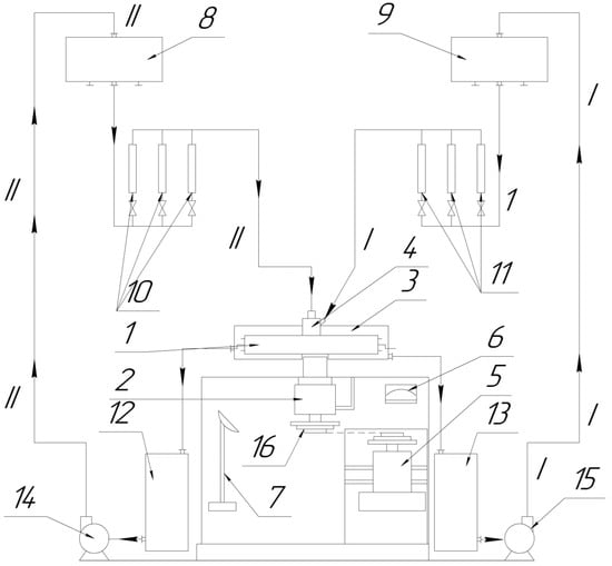
Figure 1. Schematic diagram of the experimental setup.

The shaft of the bearing assembly is driven by an electric motor (5) via a V-belt drive. Various rotation speeds were achieved using a set of interchangeable pulleys (16). The rotor speed was monitored by a mechanical tachometer and a stroboscopic tachometer (6) (ST-5, Analitpribor R&D Association, Tbilisi, Georgia). These optical and mechanical measurement methods were deliberately selected to avoid the use of electronic sensors with slip rings (current collectors), which were found to introduce significant signal distortion due to electromagnetic interference in the presence of conductive liquids. The pulsed light of the latter was used for visual observation of the process, measuring liquid levels in the apparatus and nozzles, and for photography.

Carbon tetrachloride (Zkos-1 JSC, Moscow, Russia), glycerol (Samaramedprom JSC, Samara, Russia), kerosene (Arikon Petrochemical Company JSC, Moscow, Russia), and a surfactant (ETS Group, Saint Petersburg, Russia) were used as working fluids in the experiments. Liquid supply was carried out through a special feed unit (4) and controlled by three pairs of rotameters (RS-3, RS-5, and RS-7, Teplopribor Group, Moscow, Russia; items 10, 11) for the light (line I) and heavy (line II) phases, respectively (see Figure 1). The liquids overflowed from receiving tanks (12 and 13, for the light and heavy phases, respectively) via pumps (14 and 15) into upper head tanks (8 and 9), from which they were fed through rotameters (10 and 11) into the apparatus (1).

The apparatus is a flat cylindrical rotor made of Perspex, comprising a body, a cover, a disperser with nozzles, threaded tubes for adjusting the main phase interface level, and steel tie bolts. The disperser was centered in the rotor by a circular locating ledge and secured with screws. Sealing was achieved using paronite and rubber rings.

The nozzles, as mentioned above, were installed on the disperser (Figure 2). Depending on this, the disperser was made as a cylinder with either a thin or a thick wall. Both the disperser and the efflux nozzles were made of Perspex, allowing for visual observation of the efflux process, measurement of liquid levels, and photography. Nozzles of this type are easy to manufacture and install. Pressure losses in centrifugal devices are not limited. Such nozzles are widely used in heavy-phase feed units and phase dispersion devices during the transition between transfers in the contact zone.

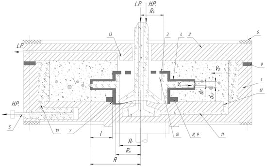
Figure 2. Scheme of transition from heavy phase to light phase.

To measure the liquid levels inside the nozzle, disperser, and apparatus, graduation marks were applied on their surfaces bordering the liquids whose levels were measured (Figure 2). To prevent the marks from influencing the efflux regime, they were filled with paint and, after drying, polished again.

The description of Figure 1 is presented in Table 1, and geometric dimensions of the investigated nozzle are presented in Table 2.

Table 1. Description of Figure 1.

Position	Designation	Description
I	Light phase	-
II	Heavy phase	-
1	Transparent model of a centrifugal machine	Transparent experimental vessel made of Plexiglas, in which the nozzles under investigation are installed
2	Bearing assembly	Vertical shaft with bearings in the housing on which the rotor is mounted
3	Steel casing	Protects the researcher, has two chambers for separate drainage of light and heavy phases
4	Special power supply unit	Device for separate phase feeding into the outlet of an experimental vessel
5	Electric motor	Drives the shaft through a V-belt transmission
6	Stroboscopic tachometer	Rotor speed measurement, illumination for observation and filming
7	Stroboscope lamp	Special lighting for observation and filming
8	Upper pressure tank for light phase	Where the light phase is fed through rotameters into the apparatus
9	Upper pressure tank for heavy phase	Where the heavy phase is fed through rotameters into the apparatus
10	Light-phase rotameters (RS-3, RS-5, RS-7)	Three pairs of rotameters for line I (light phase)
11	Heavy-phase rotameters (RS-3, RS-5, RS-7)	Three pairs of rotameters for line II (heavy phase)
12	Light-phase receiving tank	Excess light phase flows here
13	Receiving tank (or drain port) for heavy phase	The heavy phase is drained through the adjustment tubes.
14	Light-phase pump	Pumps the light phase from receiving tank 12 to pressure tank 8
15	Heavy-phase pump	Pumps the heavy phase from the receiving tank to the pressure tank 9
16	Replaceable pulleys	Allow changing the rotor speed

Table 2. Geometric dimensions and configuration of the cylindrical nozzle.

№	d0	dout	R	l	Rin
	m	m	m	m	m
1	0.001	0.01	0.104	0.044	0.06
2	0.002	0.01	-	-	-
3	0.003	0.01	0.104	0.044	0.06
4	0.004	0.01	-	-	-
5	0.005	0.01	-	-	-
6	0.006	0.01	-	-	-
7	0.007	0.01	-	-	-
8	0.008	0.01	-	-	-
9	0.002	0.004	0.104	0.02	0.06
10	-	0.006	-	-	-
11	-	0.008	-	-	-
12	-	0.001	-	-	-
13	-	0.012	-	-	-
14	-	0.014	-	-	-
15	0.002	0.01	0.075	0.015	0.06
16	-	-	0.085	0.025	-
17	-	-	0.105	0.045	-
18	-	-	0.12	0.06	-
19	-	-	0.13	0.07	-
20	-	-	0.15	0.08	-

3. Experimental Methodology

3.1. Apparatus and Materials

At the beginning of an experiment, the required rotor speed was set using the electric motor (5), interchangeable pulleys (16), and the stroboscopic tachometer (6) (see Figure 1). A small amount of the heavy phase was then fed into the apparatus to create a hydraulic seal in front of the drain hole, after which the apparatus was filled with the light phase.

The position of the Main Phase Interface (MPI) was adjusted using threaded tubes. By screwing these tubes in or out, the position of the MPI at the light-phase inlet ports of the apparatus was maintained.

Then, rotameters 11 (see Figure 1) were used to set the flow rate of the heavy phase, which passed through the supply unit into the dispersion cup with nozzles. Due to the fact that the diameter of the opening d₀ is smaller than the inner diameter of the nozzle d_out (d₀ < d_out), a layer of the flowing heavy phase ΔR = R − R₁ formed in the nozzles. R₁—the inner radius of the heavy-phase layer formed within the nozzles, defining the boundary where the heavy phase interfaces with the light phase or apparatus structure. It is adjusted via heavy-phase flow rate to match specified markings on the disperser cover and nozzle, contributing to the layer thickness (where R is the outer radius). R_s—the inner radius of the annular light-phase layer in the disperser during “open efflux cavity” mode, when ports allow light-phase entry. This creates a layer thickness ΔR_s = R₁ − R_s, which rotates with the disperser and applies additional centrifugal pressure to the heavy phase. Due to the centrifugal pressure developed by this layer, the heavy phase flowed into the light medium.

After passing through the layer of the light phase, the heavy phase reached the MPI, where it coalesced and was discharged from the rotor as a continuous stream through the threaded regulating tubes.

The excess light phase, displaced by the heavy phase, was removed from the apparatus through port (13).

In the case of countercurrent flow of the light phase, the latter was continuously fed into the MPI. From there, it moved towards the center of the rotor, thereby creating a velocity head in front of the nozzle, and upon reaching the port, it flowed out of the rotor. As mentioned above, to enable these two modes of efflux, the disperser cover (3) was equipped with ports. When these ports were closed, the case of a closed efflux cavity was observed. Otherwise, the light phase entered the disperser, forming an annular layer with a thickness of ΔR_s = R₁ − R_s. This layer, rotating with the disperser, remained stationary, creating additional centrifugal pressure on the layer of the effluxing heavy phase, i.e., the case of an open efflux cavity was observed.

By adjusting the heavy-phase flow rate, the specified value R₁ was achieved, which corresponded to the mark on the disperser cover and nozzle. Upon reaching a steady state (ΔR = const), the values of ΔR, ΔR_s, and the flow rates of the phases fed into the rotor were recorded. The values of ΔR and ΔR_s were measured against a scale inscribed inside the nozzle and on the disperser cover. Each test was repeated three times.

Distance R₁ was set prior to the experiment and visually checked to ensure that the boundary of the heavy phase was in the correct position. To verify this, control measurements were taken using photography, which differed from the visual measurements by ±2%, so the R₁ values can be considered reliable. During the experimental studies, the flow process was studied in nozzles whose configurations and geometric parameters are presented in Table 1 and Table 2.

3.2. Experimental Procedure

The studies were conducted using various liquids, whose physicochemical properties are presented in Table 3. When selecting systems for the experiment, it was considered that hydrocarbons are used during the extraction stage to obtain rare earth elements from aqueous solutions. One of the main extractants is tributyl phosphate, but mixtures can also be used. The lightest carrier phase in this case is decane. The density of the organic phase can therefore vary from 730 to 980 kg/m³, and the viscosity from 2 to 3.5 mPa∙s. The aqueous phase is usually a solution of rare earth element salts in either an acidic or neutral medium. The density of the aqueous phase, depending on the salt concentration, can vary from 1050 to 1700 kg/m³. However, the main density range is from 1200 to 1550 kg/m³. The viscosity can vary from 1 to 10 mPa∙s. Before conducting the experiment, the liquids were preliminarily mixed to an equilibrium state to exclude the possible influence of mass transfer on the flow process.

Table 3. Initial data for the experiment.

№	System	${\mathit{\rho }}_{\mathit{s}}$	${\mathit{\rho }}_0$	${\mathit{\mu }}_{\mathit{s}}$	${\mathit{\mu }}_0$	${\mathit{\sigma }}_0 \times {10}^{-3}$
-	Light Phase–Heavy Phase	$\left(\frac{\mathbf{k}\mathbf{g}}{{\mathbf{m}}^3}\right)$	$\left(\frac{\mathbf{k}\mathbf{g}}{{\mathbf{m}}^3}\right)$	$\left(\mathbf{m}\mathbf{P}\mathbf{a}·\mathbf{s}\right)$	$\left(\mathbf{m}\mathbf{P}\mathbf{a}·\mathbf{s}\right)$	$\left(\frac{\mathbf{N}}{\mathbf{m}}\right)$
	(LP–HP)
1	Kerosene–water	804	1000	1.1494	1.143	29.77
2	Water–carbon tetrachloride	1000	1593	1.1436	0.947	35.30
3	Water–78% CCl4 + 22% kerosene	1000	1410	1.1436	0.961	24.24
4	Water–68% CCl4 + 32% kerosene	1000	1315	1.1436	0.972	32.05
5	Water–45% CCl4 + 55% kerosene	1000	1205	1.1436	0.993	30.11
6	Water–37% CCl4 + 63% kerosene	1000	1098	1.1436	1.102	29.03
7	Kerosene–78% glycerol + 22% water	804	1198	1.494	45.30	12.97
8	Kerosene–70% glycerol + 27% water	804	1185	1.494	32.40	12.55
9	Kerosene–71% glycerol + 29% water	804	1179	1.494	25.54	12.89
10	Kerosene–67% glycerol + 33% water	804	1160	1.494	17.30	11.40
11	Kerosene–60% glycerol + 40% water	804	1147	1.494	10.83	11.02
12	78% glycerol + 22% water–CCl4	1193	1593	45.3	0.947	12.97
13	73% glycerol + 27% water–CCl4	1190	1593	32.4	0.947	12.55
14	71% glycerol + 29% water–CCl4	1177	1593	25.54	0.947	11.89
15	67% glycerol + 33% water–CCl4	1160	1593	17.3	0.947	11.40
16	Kerosene–water + 0.018 g/L surfactant	804	1000	1.494	1.132	29.38
17	Kerosene–water + 0.018 g/L surfactant	804	1000	1.494	1.116	20.80
18	Kerosene–water + 0.04 g/L surfactant	804	1000	1.494	1.102	9.16

Before conducting the experiment, the physicochemical properties of the substances were measured. The density was determined by the areometric method, in accordance with GOST 18995.1-73 [17]. The viscosity was determined by a capillary viscometer, in accordance with GOST 33452-2015 [18]. The interfacial tension was determined by the platinum ring tear method—the Du Nouy method.

3.3. Measurement Error

The diameters of the holes d₀ and d_out were measured with an accuracy of ±0.1 mm, and the distances R and R₁ were measured with an accuracy of ±0.5 mm. Before conducting a series of experiments with different media, the rotameters were calibrated using these media. Next, a calibration table was constructed, which was used to determine the flow rate. In accordance with the accuracy class of the device, the error does not exceed 5%. The angular velocity of the experimental vessel was determined by the readings of a stroboscope. In accordance with the accuracy class of the device, the error does not exceed 0.2%.

In addition to instrumental uncertainties, several other sources of error should be acknowledged. Human-related uncertainties associated with visual determination of liquid levels and steady-state conditions are unavoidable in laboratory experiments; however, their influence was minimized by conducting all measurements under stable operating regimes, repeating each experiment three times, and verifying critical distances using photographic control. Similar approaches to mitigating human and procedural uncertainties in experimental measurements are widely discussed in the literature [19,20,21].

The experimental data inevitably contain random noise arising from flow fluctuations, optical reading resolution, and calibration limits of the measuring devices. These effects contribute to data scatter and affect regression-based fitting; however, their impact is reflected in the reported determination coefficients and residual errors of the fitted correlations [22,23].

Finally, it should be noted that although numerical modeling and CFD-based uncertainty quantification are not the subject of the present work, the experimental dataset obtained here is intended to serve as a reference basis for future numerical validation studies, where modeling uncertainties can be addressed using established probabilistic and multi-fidelity approaches [21,23].

4. Results

4.1. Experiment Results

The results of numerous empirical experiments conducted on the installation are presented in Table 4, Table 5 and Table 6.

Table 4. Results of the experiment. System 1.

№	d0	dn	ω	R	ΔR	ΔRs	Rs	Q0 × 10−5
-	(mm)	(mm)	(s−1)	(mm)	(mm)	(mm)	(mm)	(m3/s)
1	1.5	10	91.5	104	54	0	67	0.718
2	2	10	91.5	104	54	0	67	1.252
3	3	10	91.5	104	54	0	67	2.510
4	4	10	91.5	104	54	0	67	4.100
5	5	10	91.5	104	54	0	67	6.128
6	6	10	91.5	104	54	0	67	8.340
7	1.5	10	131	104	54	0	67	0.960
8	2	10	131	104	54	0	67	1.663
9	3	10	131	104	54	0	67	3.400
10	4	10	131	104	54	0	67	5.426
11	5	10	131	104	54	0	67	8.000
12	6	10	131	104	54	0	67	11.170
13	1.5	10	183	104	54	0	67	1.270
14	2	10	183	104	54	0	67	2.191
15	3	10	183	104	54	0	67	4.500
16	4	10	183	104	54	0	67	7.525
17	5	10	183	104	54	0	67	10.850
18	6	10	183	104	54	0	67	15.410
19	2	4	91.6	104	54	0	67	1.010
20	2	8	91.6	104	54	0	67	1.188
21	2	10	91.6	104	54	0	67	1.257
22	2	12	91.6	104	54	0	67	1.275
23	2	4	131	104	54	0	67	1.495
24	2	8	131	104	54	0	67	1.548
25	2	10	131	104	54	0	67	1.669
26	2	12	131	104	54	0	67	1.751
27	2	4	183	104	54	0	67	1.950
28	2	8	183	104	54	0	67	2.036
29	2	10	183	104	54	0	67	2.220
30	2	12	183	104	54	0	67	2.320
31	2	10	91.6	104	54	0	67	1.249
32	2	10	131	104	54	0	67	1.693
33	2	10	157	104	54	0	67	1.850
34	2	10	183	104	54	0	67	2.285
35	2	10	209	104	54	0	67	2.310
36	2	10	261.6	104	54	0	67	2.750
37	2.5	10	107.8	85	36	0	62	1.931
38	2.5	10	107.8	85	41	0	62	2.130
39	2.5	10	107.8	85	50	0	62	2.390
40	2.5	10	107.8	85	62	0	62	2.497
41	2.5	10	157	85	36	0	62	2.680
42	2.5	10	157	85	41	0	62	2.910
43	2.5	10	157	85	50	0	62	3.160
44	2.5	10	157	85	62	0	62	3.380
45	2.5	10	210.38	85	36	0	62	3.440
46	2.5	10	210.38	85	41	0	62	3.710
47	2.5	10	210.38	85	50	0	62	4.169
48	2.5	10	210.38	85	62	0	62	4.423
49	2	10	91.6	0.08	54	0	67	1.579
50	2	10	91.6	0.09	54	0	67	1.340
51	2	10	91.6	0.1	54	0	67	1.270
52	2	10	91.6	0.12	65	0	67	1.233
53	2	10	91.6	0.14	75	0	67	1.175
54	2	10	131	0.08	54	0	67	2.125
55	2	10	131	0.09	54	0	67	2.015
56	2	10	131	0.1	54	0	67	1.772
57	2	10	131	0.12	65	0	67	1.689
58	2	10	131	0.14	75	0	67	1.634
59	2	10	183	0.09	54	0	67	2.662
60	2	10	183	0.1	54	0	67	2.285
61	2	10	183	0.12	65	0	67	2.264
62	2	10	131	104	54	5	62	1.597
63	2	10	131	104	54	10	62	1.714
64	2	10	131	104	54	15	62	1.733
65	2	10	131	104	54	20	62	1.868
66	2	10	131	104	54	25	62	1.870

Table 5. Experimental results for systems 1–8.

№	d0	dn	ω	R	ΔR	ΔRs	Rs	Q0 × 10−5
-	(mm)	(mm)	(s−1)	(mm)	(mm)	(mm)	(mm)	(m3/s)
System №1
67	2	10	96.1	104	54	0	67	1.25
68	2	10	131	104	54	0	67	1.69
System №2
69	2	10	91.6	104	54	0	67	1.5
70	2	10	131	104	54	0	67	2.08
71	2	10	183	104	54	0	67	2.8
System №3
72	2	10	91.6	104	54	0	67	1.44
73	2	10	131	104	54	0	67	1.97
74	2	10	183	104	54	0	67	2.63
System №4
75	2	10	91.6	104	54	0	67	1.32
76	2	10	131	104	54	0	67	1.81
77	2	10	183	104	54	0	67	2.44
System №5
78	2	10	91.6	104	54	0	67	1.26
79	2	10	131	104	54	0	67	1.77
80	2	10	183	104	54	0	67	2.36
System №6
81	2	10	91.6	104	54	0	67	1.14
82	2	10	131	104	54	0	67	1.58
83	2	10	183	104	54	0	67	2.16
System №7
84	2.2	10	157	104	57	0	65	3.1
85	2.2	10	210.38	104	57	0	65	4.07
System №8
86	2.2	10	157	104	57	0	65	2.91
87	2.2	10	210.38	104	57	0	65	3.85

Table 6. Experimental results for systems with 9–18.

№	d0	dn	ω	R	ΔR	ΔRs	Rs	Q0 × 10−5
-	(mm)	(mm)	(s−1)	(mm)	(mm)	(mm)	(mm)	(m3/s)
System №9
88	2.2	10	157	105	57	0	65	2.74
89	2.2	10	210.38	105	57	0	65	3.54
System №10
90	2.2	10	157	105	57	0	65	2.64
91	2.2	10	210.38	105	57	0	65	3.45
System №11
92	2.2	10	157	105	57	0	65	2.56
93	2.2	10	210.38	105	57	0	65	3.27
System №12
94	2.2	10	107.8	105	57	0	65	1.65
95	2.2	10	210.38	105	57	0	65	2.88
System №13
96	2.2	10	107.8	105	57	0	65	1.74
97	2.2	10	210.38	105	57	0	65	3.04
System №14
98	2.2	10	107.8	105	57	0	65	1.82
99	2.2	10	210.38	105	57	0	65	3.18
System №15
100	2.2	10	107.8	105	57	0	65	1.9
101	2.2	10	210.38	105	57	0	65	3.25
System №16
102	2	10	96.1	104	54	0	67	1.23
103	2	10	131	104	54	0	67	1.63
System №17
104	2	10	96.1	104	54	0	67	1.24
105	2	10	131	104	54	0	67	1.59
System №18
106	2.1	10	96.1	104	54	0	67	1.19
107	2.1	10	131	104	54	0	67	1.61

The following notation is used in this study: d₀ is the diameter of the inlet opening, d_n is the inner diameter of the nozzle, ω is the angular velocity of the rotor, R is the outer radius of the heavy-phase layer, R₁ is the inner radius of this layer, and R_s is the radial position of the light-phase boundary formed under open discharge conditions. The thickness of the heavy-phase layer is defined as ΔR = R − R₁, while the thickness of the annular light-phase layer is ΔR_s = R₁ − R_s. The heavy-phase flow rate is denoted by Q₀ (scaled by a factor of 10⁻⁵).

4.2. Discussion of Results

Initially, we examined in detail the individual influences of key parameters on the flow rate of the heavy phase from the nozzle in a centrifugal field: centrifugal force $F_{cf}$, hole diameter $d_0$, dynamic viscosity ${\mu }_c$ of the receiving medium, dynamic viscosity ${\mu }_o$ of the flowing phase, interfacial tension ${\sigma }_0$, and density of the flowing phase ${\rho }_0$. The analysis was based on the approximation of experimental data by power functions of the form $V_0=a·X^b$, where X is a variable parameter, using the least squares method (LSM). This allowed us to establish sublinear, inverse, or positive dependencies with high coefficients of determination ${\mathrm{R}}^2$ > 0.92 in most cases.

However, to increase the practical value of the model and take into account synergistic effects, it is necessary to switch to a multi-parameter approximation. Such a model integrates all significant factors into a single regression dependence, minimizing the number of parameters and providing convenience for engineering calculations in mass transfer and mass transfer processes in centrifugal extractors. The choice of a power form for the multi-parameter model is justified by the following considerations:

• Physical adequacy: zero values of independent variables (e.g., $F_{cf}=0$ or $d_0=0$) lead to $V_0=0$, which corresponds to the absence of leakage.
• Absence of extrema during extrapolation, which is critical for prototyping and digital twins of centrifugal systems.
• Minimum number of coefficients determined by LSM, with the possibility of interpolation over a wide range of parameters.

By flow rate (outflow velocity), we refer to the average volumetric flow rate, defined as the ratio of the measured flow to the cross-sectional area of the opening. To determine how the flow rate depends on the physicochemical properties of the medium and on the technological and design parameters, each factor was analyzed by varying it independently while keeping the remaining parameters fixed. The parameters considered include the centrifugal force and the diameter of the opening, while the relevant properties of the medium comprise its viscosity and the densities of the heavy and light phases.

A power-law function was chosen to represent the relationship between the flow rate and these parameters. This functional form is widely used in engineering correlations, requires only a limited number of fitting coefficients, and provides monotonic behavior when extrapolated beyond the tested range. Importantly, it allows the model to satisfy the physically expected condition that the flow rate tends to zero when either the centrifugal force or the opening diameter approaches zero.

Multiparametric approximation was performed on a complete array of experimental data (systems No. 1–18, nozzle diameters from 1.5 to 6 mm, angular rotation speeds from low to high). The general form of the model is as follows:

$$V_0=k\cdot {F_{cf}}^{b1}\cdot d_0^{b2}\cdot {{\mu }_s}^{b3}\cdot {{\mu }_0}^{b4}\cdot {{\sigma }_0}^{b5}\cdot {{\rho }_0}^{b6}$$

(1)

where k is the pre-exponential coefficient; b_i are exponents reflecting the sensitivity of V₀ to each factor. The centrifugal force is defined as F_cf = Δρω²rΔR, where Δρ = ρ₀ − ρ_s (the difference in phase densities), ΔR is the thickness of the heavy-phase layer, ω is the angular velocity, and r is the rotor radius (taking Δρ into account excludes the separate consideration of ρ_s). The remaining parameters are given in Table 3.

4.3. Approximation Procedure and Exclusion of Insignificant Parameters

The approximation was performed in logarithmic coordinates for linearization:

$$ln\left(V_0\right)=ln\left(k\right)+b_{1}ln\left(F_{cf}\right)+b_{2}ln\left(d_0\right)+b_{3}ln\left({\mu }_c\right)+b_{4}ln\left({\mu }_0\right)+b_{5}ln\left({\sigma }_0\right)+b_{6}ln\left({\rho }_0\right)$$

(2)

Using least squares method in the MATLAB (version R2024a (24.1)) programming environment. The initial model included all parameters. The coefficients of determination and significance (according to Student’s t-test at p < 0.05) were evaluated iteratively. The approximation equation itself, including all power coefficients, will take the form:

$$V_0=0.017{F_{cf}}^{0.41}{d_0}^{-0.4}{{\mu }_s}^{-0.08}{{\mu }_0}^{0.01}{{\rho }_0}^{-0.2}{{\rho }_s}^{0.01}{\sigma }^{0.02}$$

(3)

Results of the complete model:

• R² = 0.86, root mean square error (RMSE) = 8.75%.
• Significant indicators: $b_1\approx 0.41$ (for $F_{cf}$, sublinear dependence, as in one-dimensional analysis); $b_2\approx -0.39$ (inverse dependence on $d_0$ associated with an increase in hydraulic resistance and a transition to droplet mode).
• Insignificant: $b_3\approx -0.08$ (${\mu }_c$, slight deceleration); $b_4\approx 0.05$ (${\mu }_0$, laminar flow inside the nozzle); $b_5\approx 0.18$ (${\sigma }_0$, minimization of the jet surface); $b_6$ integrated into $F_{cf}$.
• An increase in the viscosity of the medium reduces the flow rate, which is consistent with the physical picture. The viscosity of the flowing phase has a negligible effect on the flow rate. Its change can be neglected and excluded from the equation.

Based on the significance analysis (contribution < 5% to the variance $V_0$), the parameters ${\mu }_0,{\sigma }_0$ and the separate term ${\rho }_0$ are excluded. Viscosity ${\mu }_c$ is retained as a weak but statistically significant factor of resistance of the surrounding phase. This is consistent with physics: the dominant influence is exerted by the driving force ($F_{cf}$), the design parameter ($d_0$) and viscous drag in the receiving medium. The approximation results are shown in Figure 3.

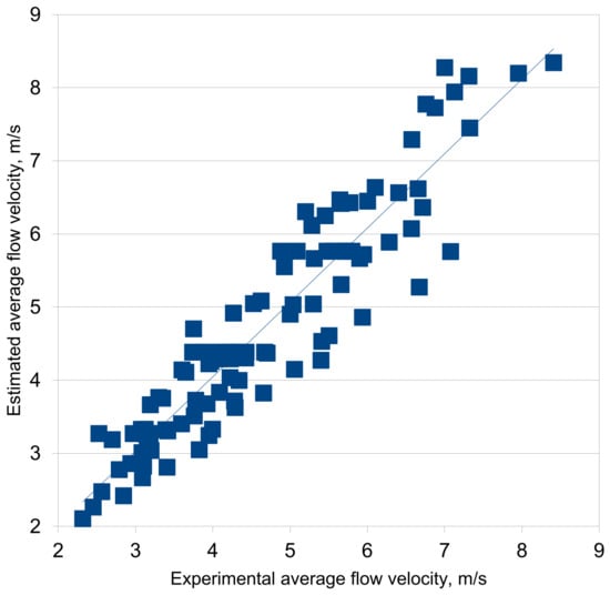
Figure 3. Results of multiparametric approximation.

Similarly, the effect on the flow rate of interfacial tension is negligible. The influence of the density of the medium should be considered only in centrifugal force.

Then we finally obtain:

$$V_0=0.015{F_{cf}}^{0.41}{d_0}^{-0.4}{{\mu }_s}^{-0.08}{{\rho }_0}^{-0.2}$$

(4)

The coefficient of determination R² = 0.87, and the standard deviation is 8.85%.

Figure 3 shows a comparison of experimental points V₀ with predictions of a simplified model (approximation line). The points are scattered symmetrically about the line, with maximum deviations in the high F_cf region (transition to turbulent flow), which is within the measurement error (±5–7%).

Physical interpretation:

• F_cf dominance: The b₁ ≈ 0.41 index is close to the 0.40–0.44 range from the one-dimensional analysis, confirming sublinearity (not $V_0\propto \sqrt{F_{cf}}$ as in Torricelli’s gravitational field, but weaker due to viscous losses and drop deformation in a centrifugal field).
• Influence of d₀: The inverse dependence (b₂ < 0) is explained by the increase in inertial losses and the transition from jet to droplet mode (increase in Weber number at low do).
• Viscosity μ_s: A weak inverse relationship (b₃ ≈ −0.08) reflects the inhibition of droplet separation by the surrounding flow of the light phase; at μ_s > 40 mPa∙s, V₀ decreases by 15–20%.
• Exclusion of μ₀, σ₀, ρ₀: Their contribution is < 3% in multidimensional regression; ρ₀ is taken into account in Δρ. This simplifies the model for digital twins without loss of accuracy.

The model is applicable in the range F_cf = 4500–115,000 N/m², d₀ = 1.5–6 mm, μ_s = 1–45 mPa∙s. For extrapolation, validation on neural network models (e.g., using CFD data for prototyping) is recommended.

5. Discussion

Analysis of experimental data showed that the velocity of liquid flow through nozzles in a centrifugal field can be satisfactorily approximated by a power function of the centrifugal force F_cf. However, the exponent at F_cf turned out to be about 0.41, which is lower than the classical value of 0.5 (which is characteristic of gravitational flow, where the velocity is proportional to √g). This difference can be explained by the influence of the Coriolis force: the rotational motion and the associated Coriolis force distort the flow profile, leading to partial deformation of the jet and a decrease in its acceleration along the direction of flow. In other words, the lateral deflection of the flow under the action of Coriolis reduces the effect of the applied centrifugal force [13,14].

When studying the rheological properties, it was found that:

• With an increase in the dynamic viscosity of the environment, the flow velocity monotonically decreases. This corresponds to the physical interpretation: an increase in viscosity increases the resistance to flow. slowing down the drop [3,14].
• Conversely, as the viscosity of the flowing liquid itself increases, the flow rate increases. This effect may be associated with the laminarization of the jet, a decrease in internal vortices, and flow stabilization, which is especially pronounced under the action of a directed centrifugal force [15,16].

As for density ${\rho }_0$, the degree of influence is primarily reflected in centrifugal force. However, it has been found that the degree of its influence is less than in centrifugal force [3,15,16].

Interfacial tension σ₀ had a positive but insignificant effect on the flow velocity. The degrees obtained in the approximation and the small increase in velocity when σ₀ changes suggest that this factor can be neglected in engineering calculations at moderate surface tension values [15,16].

The multi-parameter power model in Equation (4) adequately describes flow in a centrifugal field (R² = 0.87), integrating dominant factors and enabling engineering calculations of mass transfer. Simplification increases robustness for digital twins of centrifugal devices.

6. Conclusions

• Centrifugal force: The flow velocity of a liquid in a centrifugal field is described by a power-law dependence on the applied centrifugal force. The exponent is approximately 0.41, which is lower than the classical value of 0.5; this deviation is hypothesized to be due to the influence of the Coriolis force.
• Phase viscosity: An increase in the dynamic viscosity of the surrounding (receiving) phase leads to a decrease in the flow velocity. At the same time, an increase in the viscosity of the flowing liquid itself can be neglected.
• Surface tension: This factor has only a slight positive effect on the flow process and can be ignored in modeling in the range σ₀ ≈ 10–30 mN/m, since a change in the limits leads to a change in velocity of no more than 2%.
• Fluid density: The effect of the density of the flowing fluid is exponential (exponent −0.2) and falls within the experimental error range. Thus, the change in density is effectively taken into account by the basic exponential model without the need for special corrections. The density of the medium should only be taken into account in the value of the centrifugal force.
• Thus, the main parameters determining the flow regime of a liquid in a centrifugal field are centrifugal acceleration and the rheological properties of both phases (primarily viscosity). The contribution of surface tension is secondary under the conditions considered and can only be taken into account when fine-tuning the model is necessary. The results obtained can be used to verify numerical flow models. in the design of centrifugal mass transfer devices and in the evaluation of their performance.

References

- Fedorov, A.T. Investigation of the Separation of Ytterbium, Yttrium, Erbium, and Iron during Their Re-Extraction from D2EGPhA Solutions. Probl. Nedropolz. 2018, 249–251. Available online: https://spmi.ru/sites/default/files/imci_images/sciens/nirs/vkladka_2_%D1%87%D0%B0%D1%81%D1%82%D1%8C%20II_%202018.pdf (accessed on 6 January 2026).
- Krasil’nikov, A.Y.; Politov, Y.A. Centrifugal Extractors with Magnetic Coupling for Radiochemical and Chemical Productions. At Energy 2014, 117, 123–129. [Google Scholar] [CrossRef]
- Eggert, A.; Sibirtsev, S.; Menne, D.; Jupke, A. Liquid–Liquid Centrifugal Separation—New Equipment for Optical (Photographic) Evaluation at Laboratory Scale. Chem. Eng. Res. Des. 2017, 127, 170–179. [Google Scholar] [CrossRef]
- Gómez-Pérez, C.A.; Espinosa, J. The design analysis of continuous bioreactors in series with recirculation using Singular Value Decomposition. Chem. Eng. Res. Des. 2017, 125, 108–118. [Google Scholar] [CrossRef]
- Hamamah, Z.A.; Grützner, T. Liquid-Liquid Centrifugal Extractors: Types and Recent Applications—A Review. Chem. Bio. Eng. Rev. 2022, 9, 286–318. [Google Scholar] [CrossRef]
- Chakma, P.; Zhao, H.; Jeon, J.; Lee, Y.W. Flow Behavior and Performance Analysis of Annular Centrifugal Contactor for Liquid–Liquid Separation: A Numerical Study. J. Adv. Mar. Eng. Technol. 2022, 46, 182–192. [Google Scholar] [CrossRef]
- Abdelnaeem, K.A.; Thévenin, D.; Zähringer, K.; Abdelsamie, A.; Mansour, M. Numerical Investigations of Liquid-Liquid Extraction through a Coiled Tube Integrated with an Extraction Outlet. Chem. Eng. Process. Process Intensif. 2025, 213, 110310. [Google Scholar] [CrossRef]
- Versteyhe, D.; Binnemans, K.; Van Gerven, T. Recent Advancements in Centrifugal Contactor Design for Chemical Processing. Curr. Opin. Chem. Eng. 2025, 47, 101084. [Google Scholar] [CrossRef]
- Maertens, D.; Binnemans, K.; Cardinaels, T. Design of a Modular Annular Centrifugal Contactor for Lab-Scale Counter-Current Multistage Solvent Extraction. Solvent Extr. Ion Exch. 2023, 41, 741–766. [Google Scholar] [CrossRef]
- Uhl, A.; Schmidt, A.; Strube, J. Digital Twin for Centrifugal Extractors Exemplified for pDNA Clarification Process after Lysis. ACS Omega 2024, 9, 31120–31127. [Google Scholar] [CrossRef] [PubMed]
- Duan, W.; Sun, T.; Zheng, Q. Development and Performance Assessment of an Industrial-Scale Modular Annular Centrifugal Contactor. Chem. Eng. J. 2025, 520, 165817. [Google Scholar] [CrossRef]
- Hamamah, Z.A.; Grützner, T. Hydrodynamics Study on Annular Centrifugal Contactors: CINC V 02 as an Example. Chem. Eng. Technol. 2023, 46, 567–578. [Google Scholar] [CrossRef]
- Kundu, P.K.; Cohen, I.M.; Dowling, D.R. Fluid Mechanics, 6th ed.; Academic Press: Cambridge, MA, USA, 2015; pp. 136–145. [Google Scholar]
- Bird, R.B.; Stewart, W.E.; Lightfoot, E.N. Transport Phenomena, 2nd ed.; John Wiley & Sons: New York, NY, USA, 2007; pp. 58–62. [Google Scholar]
- Clift, R.; Grace, J.R.; Weber, M.E. Bubbles, Drops, and Particles; Dover Publications: Mineola, NY, USA, 1978; pp. 320–350. [Google Scholar]
- Myers, R.H.; Montgomery, D.C.; Anderson-Cook, C.M. Response Surface Methodology: Process and Product Optimization Using Designed Experiments, 4th ed.; John Wiley & Sons: Hoboken, NJ, USA, 2016; pp. 13–45. [Google Scholar]
- GOST 18995.1-73; Density of Liquids. Areometric Method. Standards Publishing: Moscow, Russia, 1973.
- GOST 33452-2015; Viscosity of Liquids. Capillary Viscometer Method. Standards Publishing: Moscow, Russia, 2015.
- Hughes, I.; Hase, T. Measurements and Their Uncertainties: A Practical Guide to Modern Error Analysis; OUP: Oxford, UK, 2010. [Google Scholar]
- Baars, B.J. (Ed.) Experimental Slips and Human Error: Exploring the Architecture of Volition; Springer Science & Business Media: Berlin/Heidelberg, Germany, 2013. [Google Scholar]
- Mishra, A.A.; Mukhopadhaya, J.; Iaccarino, G.; Alonso, J. Uncertainty estimation module for turbulence model predictions in SU2. AIAA J. 2019, 57, 1066–1077. [Google Scholar] [CrossRef]
- Nigam, N.; Mohseni, S.; Valverde, J.; Voronin, S.; Mukhopadhaya, J.; Alonso, J.J. A toolset for creation of multi-fidelity probabilistic aerodynamic databases. In Proceedings of the AIAA Scitech 2021 Forum, Virtual Event, 11–15 & 19–21 January 2021; p. 0466. [Google Scholar] [CrossRef]
- Réfrégier, P. Noise Theory and Application to Physics: From Fluctuations to Information; Springer Science & Business Media: Berlin/Heidelberg, Germany, 2012. [Google Scholar]
Disclaimer/Publisher’s Note: The statements, opinions and data contained in all publications are solely those of the individual author(s) and contributor(s) and not of MDPI and/or the editor(s). MDPI and/or the editor(s) disclaim responsibility for any injury to people or property resulting from any ideas, methods, instructions or products referred to in the content. |
© 2026 by the authors. Licensee MDPI, Basel, Switzerland. This article is an open access article distributed under the terms and conditions of the Creative Commons Attribution (CC BY) license.