MDEALNS for Solving the Tapioca Starch Logistics Network Problem for the Land Port of Nakhon Ratchasima Province, Thailand

Abstract

Background: This research aimed to establish a network linked to generation, for the transport route of tapioca starch products to a land port, serving as the logistics hub of Thailand’s Nakhon Ratchasima province. Methods: The adaptive large neighborhood search (ALNS) algorithm, combined with the differential evolution (DE) approach, was used for the problem analysis, and this method was named modified differential evolution adaptive large neighborhood search (MDEALNS) is a new method that includes six steps, which are (1) initialization, (2) mutation, (3) recombination, (4) updating with ALNS, (5) Selection and (6) repeat the (2) to (5) steps until the termination condition is met. The MDEALNS algorithm designed a logistics network linking the optimal route and a suitable open/close factory allocation with the lowest transport cost for tapioca starch. The operating supply chain of tapioca starch manufacturing in the case study. The proposed methods have been tested with datasets of the three groups of test instances and the case study consisted of 404 farms, 33 factories, and 1 land port. Results: The computational results show that MDEALNS method can reduced the distance and the fuel cost and outperformed the highest performance of the original method used by LINGO, DE, and ALNS. Conclusions: The computational results show that MDEALNS method can reduced the distance and the fuel cost and outperformed the highest performance of the original method used by LINGO, DE, and ALNS.

1. Introduction

Customs, border protection, and other inspection organizations tasked with upholding the national laws that govern land ports determine whether or not there are checking stations. Land ports comprise land, structures, parking areas, and onsite streets that form inland ports. Land ports, however, are used to collect products for export to a foreign customer or end market; they operate similarly to an export border, but are located inland, within a country.

Products are transported to inland, or land, ports using vehicles, which land ports use to provide people with services and to receive cargo from inland, road, and rail transportation. This is the main objective of land ports. Loading and unloading operations are linked to transportation systems and services. In the past, harbor processes involved boarding or disembarking people from ships, which were only used for passenger services, and although this is still the case, the situation has changed. Product freight services involve handling and storage procedures. The group integration of numerous inland ports could be strengthened in the emerging multimodal transport systems, so that they become linked to transport nodes and have the function of product collection for export and import. A new freight transportation system for large containers has been developed for global trade containerization. Seaports have improved the transport system for the export of millions of containers, and has become necessary to generate a number of links with distant lands for this export. Rail, road, and inland waterway transport are included in this transport system [1,2,3]. The choice of the dry port location determines the container transport approach, empty container displacement, volume discounts, and suitable routing, which can optimize the inland logistic system [4]. The operational suitability of organizations is determined by the overall costs and total exportation, for which the multi-objective mixed-integer programming model was developed and put into practice. Several studies have investigated the management issues of dry ports, such as container optimization, container management, and container repair scheduling [5,6,7,8,9,10,11]. Strategic planning and decision making have been the main focus of researchers for the improvement of dry ports. Roso et al. [5] mention the importance of dry ports in rational apportionment, highlighting the functional relationship between a dry port and a seaport in linking operations together, such as the development of a number of spatial configuration options [12]. Previously, Rahimi et al. [13] developed an architecture for a modern transportation network based on dry ports, with a certain amount of crowd and contamination reduction. Henttu and Hilmola [14] conducted research and solved the problem of the effect of the number of dry ports on economic advantages.

However, the selection of a dry port location depends on several conditions, such as whether it is inland or international. Nguyen and Notteboom [15] mentioned an approach for the selection of a dry port for development in Vietnam, based on multiple criteria, and the main criteria included the users, investors, or operators, and considerations of the community. These criteria were analyzed using multi-attribute decision making (MADM), to rank the best dry ports, and the two dry port locations that were shown to influence economic development were in Lao Cai and Phu Tho provinces. According to [16], the factors that affect dry port allocation are techniques, technology, organizations, ecology, IT, the economy, legalities, and regulations and specifications. The analytical hierarchy process (AHP) approach has been used for the allocation of dry ports. These conditions influenced the generation of dry port locations in the strategic EU TEN-T transport-linked routes to the seaport of Rijeka. However, the increase in factors has resulted in a complex problem, and it is difficult to conduct a data analysis for the selection of suitable dry port locations. A combination of methods is an approach used to solve problems with a large number of factors. Tadić et al. [17] presented a selection of dry port terminal locations using hybrid grey and multi-criteria decision making (MCDM) based on the analytical hierarchy process (AHP) and combinative distance-based assessment (CODAS). The conceptual conditions that must be considered for the selection of dry port terminals are the environment, economy, and social sustainability. The current market conditions indicate three suitable locations for dry port terminals; namely, Zagreb, Ljubljana, and Belgrade. Additionally, [18] presented a combination of three methods, comprising a confirmatory factor analysis (CFA), a measurement of attractiveness using a categorical-based evaluation technique (MACBETH), and a preference ranking organization method for the enrichment of evaluations (PROMETHEE), in order to generate a mathematical model to solve the problem of dry port selection in southern Thailand. The railway in Phatthalung province was chosen as the new railway for dry ports, for the import and export of products. The mathematical model could effectively solve the location selection problem of dry ports and had a high level of performance.

Moreover, the improvement of the transport system in dry ports has been studied by many researchers. For example, in 2012, Monios and Wilmsmeier improved the transport system of large ships, by rebuilding the transport chain [19]. Moreover, Ambrosino and Sciomachen [20] studied the problem of the location of dry ports in multi-modal transport sections, and this led to the exploration of the transportation methods of road and rail together. In order to increase the performance of dry port locations, Wang, Chen, and Huang [21] determined a suitable location for a dry port, in an attempt to increase performance in the transport system, by closing the current dry ports in unsuitable locations and opening new ones.

All the above studies used an approach to problem solving based on mathematical programming and other mathematical models. Moreover, Wei, Hairui, and Dong [22] presented a new cross-border logistics network, which links the seafaring logistics network to the inland cross-border logistics network via dry ports. Furthermore, the organizational optimization problem has been studied, regarding the import and export of goods inland in manifold network scenarios, using the genetic algorithm (GA) method as a solution to the problem. In previous research, the split vehicle routing problem of deliveries and pickups for inland container shipping in dry-port-based systems was addressed. A local search using the greedy approach and Tabu search were used to generate a data analysis model. The results could help in the decision-making process for inland terminals [23]. Moreover, several heuristics approaches have been used for allocation and logistics problem solving and have shown high performance. For example, the modified differential evolution (MDE) algorithm based on the DE approach has been used to solve the allocation of rubber fields for latex import and the fuel consumption of trucks under different road conditions. The MDE could generate a solution 13.82% better than the original DE approach in testing [24]. The authors of [25] reported the tabu search and simulated annealing methods in the problem solving of location-inventory-routing problems in a closed-loop supply chain (LIRP-CL), with consideration of random demands and random returns from customers, to minimize the total costs of the system. This hybrid heuristic could generate network vehicle routes for product delivery, while effectively lowering the system’s total cost. Moreover, the authors of [26] created a modified version of the resistive grid path planning methodology (RGPPM) technique for planning product deliveries, so that this technique could reduce the route distance to 45% of the old route. The method of particle swarm optimization was used to solve the vehicle routing problem with cross-docking and decrease the carbon emissions in the transport of logistic systems. This method demonstrated a decrease vehicle distances, which could reduce the cost of the process for both pickup and delivery, as well as the cost of CO₂ emissions in logistic and supply chain planning [27].

An improved method has been proposed to solve the vehicle routing problem with time windows (VRPTW), with a modified choice function (MCF) based on the adaptive large neighborhood search (ALNS) method, and this is called the modified adaptive large neighborhood search (MALNS) method. In a previous study, this method showed an error in its computational results of 1.95%, making it well-suited for this problem [28]. Furthermore, in a previous study, a tourist route planning problem was solved by improving the local search based on ALNS, and this improved approach is called the MALNS approach. The result of the computations showed a high performance and a result error of 0.05%, when compared with the original method [29]. Moreover, a two-phase method, with the fuzzy c-means clustering method (FCM) and GA, was used to solve the network generation of optimal intermodal nodes and routes for transport in the Bohai Rim region. The result of the creation of this transport network increased the performance of sustainable transport in other regions of China [30]. According to the approach of hybrid and self-adaptive differential evolution (HSADE) algorithms, the multi-depot vehicle routing problem, which caused an egg distribution problem in Thailand, could be solved. This method could improve the total cost by 14.13% [31]. These computational methods modified how the solution was achieved, showing higher analysis effectiveness and accuracy than the original approach. Therefore, the determination of the method is important to find the exact solution, which is considered within complex data analyses.

The product transport routes in Thailand are linked by routes to several provinces, for export to other nations. Improvements in logistic and supply chain systems are important for the development of economic and transport infrastructure. The government of Thailand chose Nakhon Ratchasima province as the location to build a land port/dry port, so that agriculture and industrial products could be transported to the seaport on Thailand’s border [32]. Therefore, the logistics route, seaport location, and export transit path of Thailand’s border provide a link to the Nakhon Ratchasima dry port (NR-DP) [33]. Nakhon Ratchasima province is the pink area in the map displayed in Figure 1. This province was chosen as it is in the center of Northeast Thailand and has several industries, such as agriculture. Thus, many raw materials from other areas are transported to Nakhon Ratchasima province for product manufacturing and product transportation to land ports within a short distance, with low transport costs. The allocation of factory locations for the agricultural products received from farmers is necessary for production and export.

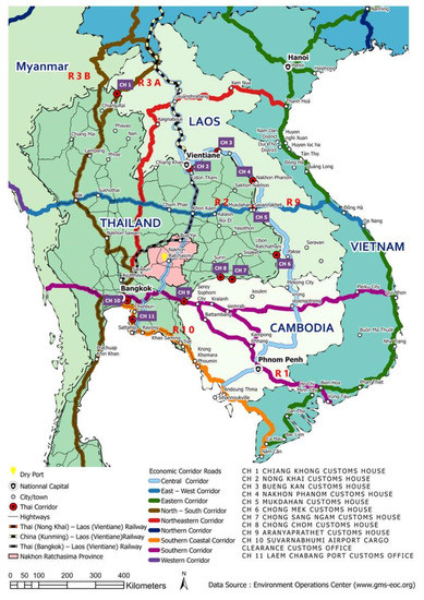
Figure 1. Transport Route of NR-DP.

However, the selection and allocation of the factory point from which goods are received from the industry and farmers is difficult, due to the optimal transport routing and costs in logistic and supply chain systems. Several factories in Nakhon Ratchasima have shown capacity performance with no differences, and farmers could not select a product transportation method for transport to a suitable factory with the lowest costs and best product damage reduction. Therefore, the product delivery for farmers should be considered. Moreover, the supply chain of exports is an industry that involves manufacturing and product transportation to land ports. Selecting a suitable route is a problem of transportation, due to the decreased costs of the logistic system, and which must not be ignored.

Therefore, this problem becomes an instance of the multi-echelon location-allocation problem. The relative linking goal of networks is to maintain a low transport cost in the supply chain. The objective and contributions of this research were the development of a new heuristic algorithm that can be used to solve the optimal network linking transport problem of NR-DP, with the lowest transport costs, and the capacity of the factory that is open/closed to receiving products, using modified differential evolution with the adaptive large neighborhood search (MDEALNS) algorithm.

This paper is organized as follows: Section 2 defines the NR-DR problem. The MDEALNS algorithm approach and computational results are presented in Section 3, Section 4 and Section 5, as well as presenting the conclusions and suggestions for further study.

2. Problem Definition of NR-DP

An important agricultural product of Northeast Thailand is cassava root, which is a raw material used in industries for the transformation of several products. Tapioca starch, manufactured from cassava roots, is a product that is transported to the market and used in the food business and directly consumed by people. In addition, tapioca starch is extensively used in the paper and textile manufacturing industries, and it is used as a constituent in products such as seasoning powder and sweeteners.

In Nakhon Ratchasima province, tapioca starch is manufactured for consumer and export products, and the supply chain of tapioca starch manufacturing consists of 404 cassava farms, 33 tapioca factories, and one land port, as shown in Figure 2.

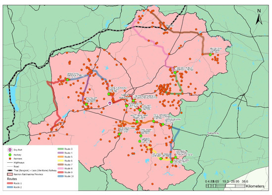
Figure 2. Locations of farmers, factories, and land port.

The farmers are dispersed around Nakhon Ratchasima, as well as the factories that receive the raw materials from these cultivators. Many agriculturists send their products to nearby factories, but each factory’s capacity has an unequal demand for raw materials. When at full capacity, the factory is closed to receiving materials. Then, the farmer must send their product to another factory that is far away, which affects the cost of product transportation and the risk of damage. Therefore, factory allocation is important for the determination of a factory that is open to receiving products in a case study. The linking of logistic networks should be considered.

Tapioca starch products have a logistics system that starts with the delivery of cassava roots from farmers to tapioca plants. Tapioca starch products are transported to a dry port and placed in a container for transport to a seaport or borders for export to other countries.

Therefore, the 404 farmers consign various cassava products to a tapioca factory, which is either open or closed to receiving the products depending on the quantity of goods from the supply farmers. Each plant has a different capacity for processing raw materials into finished products, and in areas where raw materials are uncertain, hard delivery planning [34] is used, making the selection decisions for farmers for tapioca transportation to a suitable factory difficult. This results in the problem of allocating factories as open/closed to receiving products, including the vehicle routing problem for product delivery from the farmer. A conceptual network linking tapioca starch manufacturing logistics is displayed in Figure 3.

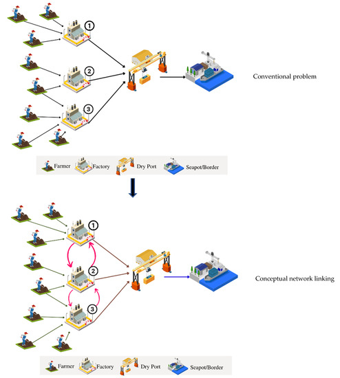
Figure 3. Conceptional framework of the considered problem.

The creation of a linked network of tapioca starch manufacturing and export should not be postponed.

3. Modified Differential Evolution with Adaptive Large Neighborhood Search

The Modified Differential Evolution with Adaptive Large Neighborhood Search (MDEALNS) method is a new meta-heuristic; its structure can be easily understood, and it presents a simple way of searching for the solution in a large area. It consists of the following six steps, based on [35]:

(1)

Initialization

(2)

Mutation

(3)

Recombination

(4)

ALNS

(5)

Selection

(6)

Repeat steps 2–5 until the termination condition is met. Figure 4 shows a flowchart of MDEALNS.

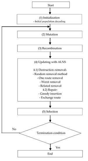Figure 4. Flow chart of MDEALNS.

3.1. Initialization

This step consists of creating the initial population to be used in the initialization of step 1, which generates a set of tracks from Table 1 by selecting track 1, as shown in Table 1.

Table 1. Initialization.

	Farmer
Factory	1	2	3	4	5
1	0.23	0.72	0.31	0.68	0.17
2	0.47	0.48	0.41	0.06	0.67
3	0.86	0.49	0.71	0.82	0.83

Initial Population Decoding

This step converts the random numbers in each of the initial vectors to become the desired objective function value, which is the total transport distance and the cost of fuel for transportation. The calculation example uses the data in Table 2.

Table 2. Initial population decoding.

Factory	1	2	3
Demand (tons)	30	40	35
Farmer	1	2	3	4	5
Production capacity (tons)	15	27	28	20	15
Capacity = 15 tons and 30 tons	Fuel cost = 35 baht/L

Note: The fuel consumption rate for 15 tons is 4 km/L, and 30 tons has a fuel consumption rate of 3 km/L.

The procedure used to convert the initial vector to the default answer is as follows:

Step 1: The components are divided into two groups; namely, (1) the factory group and (2) the farmer group, as shown in Table 3.

Table 3. Converting the initial vector.

	Farmer
	1	2	3	4	5
Factory	0.23	0.72	0.31	0.68	0.17

Step 2: The random numbers in each group are sorted, from the least to greatest, as shown in Table 4.

Table 4. Sorting random numbers.

	Farmer
	5	1	3	4	2
Factory	0.17	0.23	0.31	0.68	0.72

Step 3: Once the random numbers in each group are sorted, from the least to the greatest, farmer group 5 is assigned cassava chips to factory 1 first, and then they select trucks with capacities of 15 tons and 30 tons by selecting the size. The capacity of the car is as follows:

(1)

Vehicle size with a capacity of 15 tons requires the use of the lower bound of 0.01–0.50.

(2)

The 30-ton vehicles are required to use the upper bound of 0.51–1.00.

By choosing the size of the car capacity for the farmer group, one random 0–1 value is generated. If the random value is less than or equal to 0.05, a capacity of 15 tons is chosen; and if the random value is more than 0.05, a capacity of 30 tons is chosen. Therefore, other points are assigned in order, until the farmer makes enough deliveries to meet the needs of the factory. Table 4 presents the delivery assignment of farmer group 5, with a production capacity of 15 tons. Then, the capacity of the car is randomly selected with a random value equal to 0.03, resulting in the capacity of the car being only 15 tons, so it must be shipped to factory 1. Therefore, because factory 1 is unable to receive delivery from other farmers and has a demand of 30 tons, the demand is not met. Thus, the delivery of another farmer is assigned to group 1, because random numbers are selected from the lowest value to produce a value equal to 15 tons. The value is equal to 0.68, so a capacity of 30 tons is chosen for delivery to factory 1; and, as another 15 tons have already been received, this equals 30 tons. When the demand is met, factory 1 is closed for production. Then, deliveries are assigned to factory 2 for every farmer. We can find the objective value of this initial vector. By using the distance data in Table 5, the type of capacity data in Table 6 is used in the calculation.

Table 5. Distance matrix to convert the answer value.

		Factory			Farmer
		1	2	3	1	2	3	4	5
Factory	1	-	3	16	20	36	45	78	90
	2	3	-	18	37	41	87	98	103
	3	16	18	-	66	82	107	111	124
Farmer	1	20	37	66	-	98	121	132	144
	2	36	41	82	98	-	108	122	167
	3	45	87	107	121	108	-	98	135
	4	78	98	111	132	122	98	-	153
	5	90	103	124	144	167	135	153	-

Table 6. Capacity type matrix to convert the answer value.

		Factory			Farmer
		1	2	3	1	2	3	4	5
Factory	1	-	15 tons	15 tons	30 tons	30 tons	15 tons	15 tons	15 tons
	2	15 tons	-	30 tons	30 tons	30 tons	30 tons	15 tons	15 tons
	3	15 tons	30 tons	-	15 tons	30 tons	30 tons	30 tons	15 tons
Farmer	1	30 tons	30 tons	15 tons	-	30 tons	15 tons	15 tons	30 tons
	2	30 tons	30 tons	30 tons	30 tons	-	15 tons	30 tons	30 tons
	3	15 tons	30 tons	30 tons	15 tons	15 tons	-	15 tons	15 tons
	4	15 tons	15 tons	30 tons	15 tons	30 tons	15 tons	-	30 tons
	5	15 tons	15 tons	15 tons	30 tons	30 tons	15 tons	30 tons	-

In Table 7, the objective value is the total distance and fuel cost. By dividing the distance by the rate of fuel consumption (which depends on the capacity of the car), the result is the amount of oil used (liters), and then the fuel consumption rate can be divided by the oil price. This research was set at THB 35 per liter. The result is the cost of fuel used for each route. The sum of the overall distance objectives is 663 km, and the overall cost of fuel is THB 6349.58.

Table 7. Objective values.

No.	Route	Distance (km)	Capacity of Car (tons)	Fuel Consumption Rate (km/L)	Cost of Fuel (Baht)
1	Farmer 5-Factory 1	90	15	3	1050.00
	Farmer 1-Factory 1	20	30	4	175.00
2	Farmer 3-Factory 2	87	30	4	761.25
	Farmer 4-Factory 2	98	15	3	1143.33
3	Factory 4-Farmer 2	122	30	4	1067.50
	Farmer 2-Factory 3	82	30	4	717.50
	Factory 3-Farmer 2	82	30	4	717.50
	Farmer 2-Factory 3	82	30	4	717.50
Total of objective values.		663			6349.58

3.2. Mutation

The mutation process changes the values into coordinates, referred to as the weighting factor (F), to create a new set of results, and this method was mentioned by Price [36]. This is used to calculate the mutant vector from Equation (1), as shown in Table 8.

$$V_{i,G+1}=X_{best,G}+F(X_{r_1^i,G}-X_{r_2^i,G})+F(X_{r_3^i,G}-X_{r_4^i,G})$$

(1)

Table 8. Mutation (V_i,G+1), (F = 0.6).

	Farmer
	1	2	3	4	5
Factory 1 (Target vector (Xi,G+1))	0.23	0.72	0.31	0.68	0.17
Factory 2 (Target vector (Xi,G+1))	0.47	0.48	0.41	0.06	0.67
Factory (Mutant vector (Vi,G+1))	0.26	0.41	0.76	0.04	0.66

When using F as a weighting factor, Gämperle et al. [37] stated that a value of 0.6 for the weighting factor (F) is a good initial choice for finding appropriate answers.

Table 8 shows the determination of mutant vectors by randomly selecting five target vector values from vector 1 in Table 8 by substituting the values into Equation (1). The selected target vector must not be the same as the default vector that has already been selected to calculate the mutant vector value, which is the best answer in each model. That is, the initial vector 2 is the result of calculating the mutant vector of factory 1, which is 0.47 + 0.6(0.31 + 0.72) + 0.6(0.23 − 0.17) = 0.26, etc., where 0.47 is the best answer of the model. Then, the data in Table 8 is used, and this result is entered into the coordinate recombination process and the next selection process.

3.3. Recombination

The recombination process increases the diversity of answers, and this step provides the trial vector as in Equation (2), by means of modifying the values in the coordinates. The resulting recombination is routed as shown in Table 9. The researchers chose CR = 0.9 because Gämperle stated that CR = 0.9, which is a good starting point for finding a suitable answer.

$$U_i,G=\left\{\begin{array}{c}{X}_i^j,G otherwise\\ V_i^j,G if\left(rand\left(j\right)\le CR\right)\end{array}\right.$$

(2)

Table 9. Trial vector (U_i,G) (CR = 0.9).

Factory	Farmer
	1	2	3	4	5
Target vector random	0.03	0.63	0.97	0.32	0.39
Target vector (Xi,G+1)	0.23	0.72	0.31	0.68	0.17
Mutant vector (Vi,G+1)	0.26	0.41	0.76	0.04	0.66
Trial vector (Ui,G)	0.26	0.41	0.31	0.04	0.66

The procedure for exchanging values in coordinates (recombination) uses the binomial crossover method. Consider and compare the exchange of coordinates as shown in Equation (2) by randomly selecting numbers between 0 and 1. If the random target vector is less than or equal to the CR value, choose the value of the mutant vector. If the random target vector random value is greater than the CR value, select the target vector value. The exchange results for the coordinates are shown in Table 9.

Table 9 shows the results of the exchange procedure in coordinates using the binomial crossover method, by considering and comparing the exchange of coordinates, as shown in Equation (2). This research uses a CR = 0.9. For example, factory 1 has a random target vector of 0.03, which is less than the CR of 0.9, so choose a value for the mutant vector of 0.66, but if the random target vector is greater than CR, choose a target vector value. For example, the third farmer has a random target vector of 0.97, which is greater than a CR of 0.9, so choose a target vector of 0.31. Then, take the trial vector values to arrange the cassava transport route, as shown in Table 10, by selecting the factory with the lowest trial vector value and selecting the route first.

Table 10. Sort the trial vector values in ascending order.

	Farmer
	4	1	3	2	5
Trial vector (Ui,G)	0.04	0.26	0.31	0.41	0.66

Table 10 shows the arrangement of the trial vector (Ui,G) values, in ascending to descending order. The assignment starts with farmer group 4, and the production capacity is 20 tons. Then, randomly select the capacity of the car by randomly obtaining a car size equal to 15 tons. Only 15 tons are necessary for the delivery of farmer group 4 to factory 1. Then, return to the transport again. In order to receive more from farmer group 1, in order to meet the needs of processing factory 1, a car capacity of 30 tons is also required from farmer group 4, because farmer group 1 randomly selected a car with a capacity of 30 tons. When factory 1 receives enough cassava chips to meet the demand, then close down the factory for production. Then, assign all factories.

In Table 11, the objective value is the total distance and fuel cost. By dividing the distance by the rate of fuel consumption (which depends on the capacity of the car), the result is the amount of oil used (liters), and then the fuel consumption rate can be multiplied by the oil price. This research is set at THB 35 per liter. The result is the cost of fuel used for each route. The sum of the overall distance objectives is 743 km, and the overall cost of fuel is THB 7551.26. Then, continue with the improvement step (ALNS), as follows:

Table 11. Objective values.

No.	Route	Distance (km)	Capacity of Car (tons)	Fuel Consumption Rate (km/L)	Cost of Fuel (Baht)
1	Farmer 4-Factory 1	78	15	3	910.00
	Farmer 4-Factory 1	132	30	4	1155.00
	Farmer 1-Factory 1	20	30	4	175.00
2	Farmer 1-Farmer 3	121	15	3	1411.67
	Farmer 1-Factory 2	37	15	3	431.67
	Farmer 3-Farmer 2	108	30	4	945.00
	Farmer 2-Factory 2	41	30	4	358.75
3	Farmer 2-Factory 3	82	30	4	717.50
	Farmer 5-Factory 3	124	15	3	1446.67
Total of objective values.		743			7551.26

3.4. Adaptive Large Neighborhood Search (ALNS)

Further steps are required to improve this answer, so the researchers applied an adaptive large neighborhood search (ALNS) method. To obtain the right answer in different, wider areas, the following steps were carried out (Algorithm 1):

Algorithm 1: Algorithm of Adaptive Large Neighborhood Search

Input: problem instance I

create initial solution Smin = S ∈ S(I)

while stopping criteria not met do

for i = 1,…, pu do

select r ∈ R, d ∈ D according to probabilities p

S′ = r(d(S))

if accept(S, S′) then

S = S′

if c(S) < c(Smin) then

Smin = S

adjust the value of the current solution

Return smin

Step1 is the procedure used to generate the initial possible answer “S”. The values from the step of exchanging values in coordinates are taken as an initial set of answers, as shown in Table 12.

Table 12. Initiation of ALNS.

	Farmer
	4	1	3	2	5
Factory	0.04	0.26	0.31	0.41	0.66

Step 2 is the procedure used to determine the probability of a random initial weight, which is selected for destruction and repair with the following principles:

Substep 2.1. Destruction (removal): the researcher chooses to destroy all answer types in the four methods, as follows:

(1)

The random removal method is used to randomly select the position of the farmer or the position of the factory on the exit route, in order to rearrange the route, resulting in a pattern that destroys the answer, as shown in Figure 5.

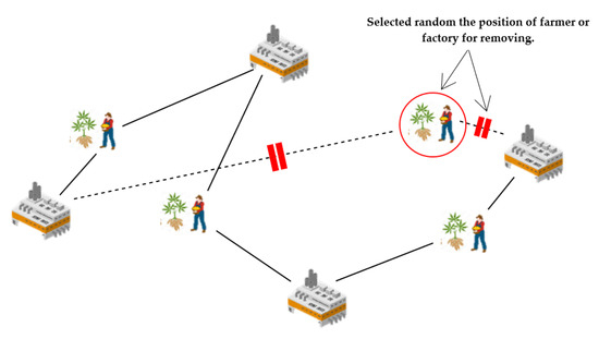Figure 5. Random removal method.

(2)

One route removal is the random destruction of a route that is separate from all the other routes, resulting in a pattern that destroys the answer, as shown in Figure 6.

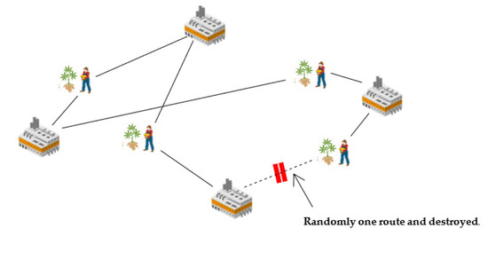Figure 6. One route removal.

(3)

Worst removal destroys the answer resulting from the worst answer of the farmer or destroys the worst answer of the factory, resulting in a pattern that destroys the answer, as shown in Figure 7.

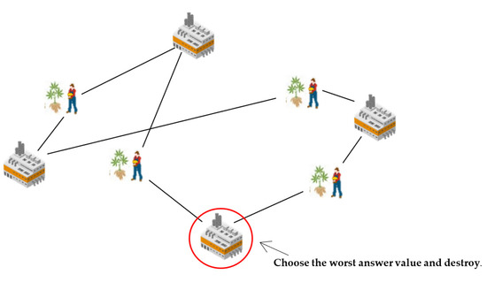Figure 7. Worst removal.

(4)

Related removal destroys the answer based on the neighboring position relative to the chosen position being destroyed, resulting in a pattern that destroys the answer, as shown in Figure 8.

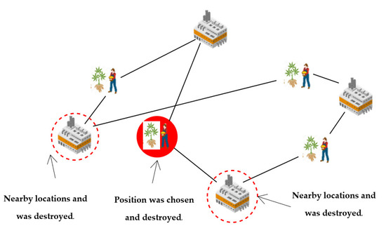Figure 8. Related removal.

Substep 2.2: To repair the answer, the researcher used two repair methods.

(1)

Greedy insertion is a method of repairing the answer by taking the difference with the lowest total distance and inserting it again, which results in a new answer, as shown in Figure 9.

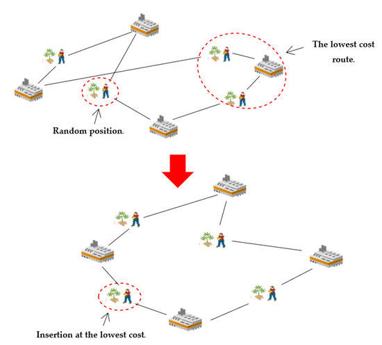Figure 9. Greedy insertion.

(2)

An exchange route is an answer repair method, which swaps the entire route for a new, lower cost route by randomly selecting a path for destruction. Once that path is removed, a new path is created, improving and, thus, repairing the answer, as shown in Figure 10.

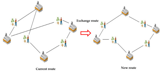Figure 10. Greedy insertion.

Step 3: Simulated annealing (SA) method for solution acceptance.

This acceptance step of ALNS has the purpose of making a decision whether to proceed with the previous answer (S) or with the new answer (S’). If the new answer (S’) shows a value worse than that of the previous answer (S), accept the new answer (S’). Moreover, recalibrate the weights to the new answer (S’). If the new answer (S’) shows a value better than that of the previous answer (S), accept the new answer (S’). All improving solutions S’ are accepted with $e^{\frac{-\left(f\left(s^{\prime }\right)-f\left(s\right)\right)}{t}}$, when t is the temperature of parameter and $f$ is objective function.

Step 4: The new solution (S’) is returned to the previous answer (S) in the next iteration by adjusting the weight and the probability of destruction until the solution is repaired; until a new, better answer is obtained; until the 100th iteration; and until a new answer is given, as in Table 13 and Table 14.

Table 13. New answer from improved (ALNS).

	Farmer
	2	1	3	5	4
Factory (Trial vector) (Ui,G)	0.41	0.26	0.31	0.66	0.04

Table 14. Objective values.

No.	Route	Distance (km)	Capacity of Car (tons)	Fuel Consumption Rate (km/L)	Cost of Fuel (Baht)
1	Farmer 2-Farmer 1	98	30	4	857.50
	Farmer 1-Factory 1	20	30	4	175.00
2	Farmer 1-Factory 2	37	30	4	323.75
	Farmer 3-Factory 2	87	30	4	761.25
3	Farmer 5-Factory 3	124	15	3	1446.67
	Farmer 4-Factory 3	111	30	4	1295.00
Total of objective values.		477			4859.17

In Table 14, the objective value is the total distance and fuel cost. By dividing the distance by the rate of fuel consumption (which depends on the capacity of the car), the result is the amount of oil used (L). The fuel consumption rate can then be multiplied by the oil price. This research is set at THB 35 per liter. The result is the cost of fuel used for each route. The sum of the overall distance objectives is 477 km, and the overall cost of fuel is THB 4859.17.

3.5. Selection

This is the process of choosing only the best answers, by comparing the function value of the trial vector that has undergone the process of improving the answer with the target vector. If the function value of the trial vector is better than the target vector, it is replaced by the next version of the trial vector, as in Equation (3), which obtains the next version to find the best answer, as in Table 15.

$$X_{i,G+1}{=}_{X_{i,G } \mathrm{Otherwise}}^{U_{i,G+1} if f\left(U_{i,G+1}\right)\le f\left(X_{i,G}\right)}$$

(3)

Table 15. Selection of responses among target vectors.

	Farmer
	5	1	3	4	2
Factory (Target vector (Xi,G))	0.17	0.23	0.31	0.68	0.72

In Table 15 and Table 16, the values of the function value of the trial vector that has undergone the improvement process and the target vector are compared. It appears that the value of the trial vector gives a better answer. Therefore, choosing a value trial vector is a good next-generation solution for finding the best solution.

Table 16. New answer from improved (ALNS).

	Farmer
	2	1	3	5	4
Factory (Trial vector (Ui,G))	0.41	0.26	0.31	0.66	0.04

3.6. Repeating

Repeat steps 2–5 until the termination condition is satisfied, which is set to be equal to 30 min.

4. Computational Results

The MDEALNS algorithm was used to solve the proposed problem and compared with LINGO version 13 software. We used Visual Studio C# for coding and simulations. The best objective was compared in cases where the optimal solution was not obtained within a limited time. The algorithms were tested for five runs, and then the best solution among the five runs was reported. Each method was set to have 30 min as the stopping criterion.

The MDEALNS algorithm was tested with datasets for three groups of test instances: (1) small-sized instances containing 5–10 farmers and 2–3 factories, which have a demand of less than 50 tons; (2) medium-sized instances containing 11–20 farmers and 4–5 factories, which have a demand of less than 100 tons, and (3) large-sized instances containing more than 21 farmers and more than 6 factories, which have a demand of more than 100 tons, including the case study problems. The computational framework is shown in Table 17.

Table 17. Details of the test instances for MDEALNS.

Instance	Farmer	Factory	Instance	Farmer	Factory
S1	5	2	M4	15	4
S2	6	2	M5	15	4
S3	7	2	L1	20	6
S4	8	3	L2	40	7
S5	9	3	L3	80	8
M1	10	4	L4	150	10
M2	10	4	L5	200	20
M3	15	4	Case study	404	33

The proposed algorithm consisted of two methods, namely, DE and ALNS. The combination of these algorithms was named MDEALNS. The details of these algorithms are shown in Table 18.

Table 18. Definition of the proposed algorithms.

Algorithm	Definition of the Proposed Algorithms
DE	Differential Evolution
ALNS	Adaptive Large Neighborhood Search
MDEALNS	Modify Differential Evolution with Adaptive Large Neighborhood Search

Datasets for Solving the Tapioca Starch Logistics Network Problem

The datasets used to solve the tapioca starch logistics network problem were tested, and the results are shown in Table 19.

Table 19. Computational results of the instance of datasets.

Instance	Lingo			Status	MDEALNS			DE			ALNS
	Distance (km.)	Fuel Cost (bath)	Time (min)		Distance (km.)	Fuel Cost (bath)	Time (min)	Distance (km.)	Fuel Cost (bath)	Time (min)	Distance (km.)	Fuel Cost (bath)	Time (min)
S1	35.6	415.3	0.06	Glo.opt	35.6	415.3	0.04	35.6	415.3	0.05	35.6	415.3	0.05
S2	57.8	674.3	0.15	Glo.opt	57.8	674.3	0.04	57.8	674.3	0.09	57.8	674.3	0.09
S3	76.3	890.2	0.05	Glo.opt	76.3	890.2	0.04	76.3	890.2	0.04	76.3	890.2	0.04
S4	88.7	1034.8	0.1	Glo.opt	88.7	1034.8	0.05	88.7	1034.8	0.06	88.7	1034.8	0.06
S5	126	1102.5	0.09	Glo.opt	126	1102.5	0.04	126	1102.5	0.08	126	1102.5	0.08
M1	187.9	1644.1	0.55	Glo.opt	187.9	1644.1	0.04	187.9	1644.1	0.15	187.9	1644.1	0.17
M2	218.4	1911	0.33	Glo.opt	218.4	1911	0.04	218.4	1911	0.18	218.4	1911	0.16
M3	285.3	3296.4	0.6	Boj *	258.6	1313.4	0.25	277.2	2925.5	0.55	279.4	3004.8	0.58
M4	293.1	3419.5	0.68	Boj *	278.3	1737.3	0.81	298.7	3213.6	0.67	305.6	3865.3	0.67
M5	333.7	4546.3	4320	Boj *	302.8	3219.9	0.73	330.4	4246.3	2.01	323.8	4022	1.87
L1	329.5	2883.1	7200	Lower Bound	308.2	1984.3	3.02	321.4	2782.3	9.67	320.1	2850.9	13.03
L2	734.2	6788.9	7200	Lower Bound	643.4	6029.5	6.13	975.9	6539.6	14.03	992.5	6689.5	16.53
L3	1067.1	10,208.4	7200	Lower Bound	843.4	9621.5	8.91	1115.9	10,721.3	15.71	1134.9	11,358.2	17.14
L4	2532.2	21,242.7	7200	Lower Bound	1275.8	16,040.5	10.23	1485.6	17,908.6	17.42	1572.8	19,389.3	19.81
L5	3644.1	31,583.2	7200	Lower Bound	2161.3	15,160.5	11.05	2665.9	24,081.6	22.16	2840.8	26,639.4	25.43
Case study	5221.34	53,301.18	7200	Lower Bound	4101.78	42,650.56	12.23	4948.18	50,512.67	26.32	5012.38	51,168.05	31.98
Average			2970.2				3.4			6.8			8.0

* Note: Opt is the optimal solution found by LINGO, Boj * is the best objective found by LINGO, and lower bound was found within 7200 min.

From Table 19, it can be seen that LINGO could find the optimal solution in the small-sized and medium-sized (M1–M2) instances, but for the medium-sized (M3–M5) instances, LINGO could only find the best objective, and in the large-sized instance case study, LINGO could only find the lower bound. However, all the proposed methods could find the optimal solution within a short time, as shown in Figure 11.

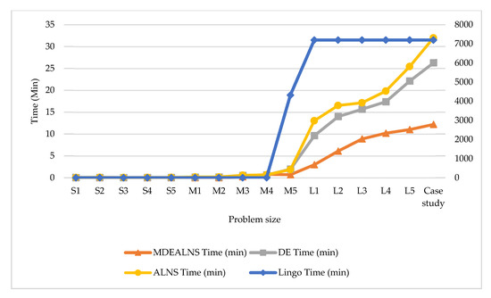
Figure 11. Comparison between the processing time of Lingo and the proposed algorithm.

The results were analyzed using statistical methods for performance comparison, as shown in Table 20 and Table 21. The results show that all methods were not significantly different when compared to the solution from LINGO.

Table 20. Statistical test results of the data distance given in Table 19.

	MDEALNS	DE	ALNS
LINGO	0.055	0.180	0.211
MDEALNS	-	0.036	0.033
DE	-	-	0.079

Table 21. Statistical test results of the data fuel cost given in Table 19.

	MDEALNS	DE	ALNS
LINGO	0.050	0.101	0.164
MDEALNS	-	0.037	0.033
DE	-	-	0.053

The results in Table 22 show that LINGO, MDEALNS, DE, and ALNS were significantly different from each other. It was found that the algorithms presented to MDEALNS, DE, and ALNS were different from the best solution provided by Lingo, which means that the proposed algorithm is effective and able to find a good answer to the proposed problems. The case study consisted of 404 farmers who were assigned to 23 factories. The aim was to minimize the distances and reduce fuel costs. The computational results of the case study when using MDEALNS are shown in Table 22 and Table 23, and Figure 12.

Table 22. Statistical test results of the data processing times given in Table 19.

	MDEALNS	DE	ALNS
LINGO	0.004	0.004	0.004
MDEALNS	-	0.010	0.012
DE	-	-	0.019

Table 23. Assignment of farmers to factories, results of the case study.

Route	Farmer	Factory	Capacity (tons)	Distance (km)	Fuel Cost (Bath)
1	1,2,3,4,5,6,7,8,9,10,11,12,13,14,15,16,17,18, 19,20,22,127,132,133,135,136,139,163,225, 226,403,404	1	15	341.76	2990.4
2	28,29,30,33,34,35,36,37,39,40,41,42,43,44, 45,46,49	2	30	157.72	1380.05
3	115,117,118,119,120,121,122,123,124,166, 178,233,234	3	30	174.51	1526.963
4	125,126,128,129,131,134,137,138,140,141, 142,143,144,145,146,147,148,149,150,151, 153,154,281	4	15	362.93	3175.638
5	130,152	5	30	58.34	510.475
6	155,156,157,161,162,277,314,315,316,317	6	30	96.51	844.4625
7	158,159,160	7	15	21.5	250.8333
8	179,180,181,182,183,184,186,187,188,189, 190,191,192,193,194,195,196,197,198,199, 200,201,202,203,204,205,206,207	8	15	135.19	1182.913
9	24,25,26,27,52,53,54,55,56,58,59,60,61,62, 64,65,67,68,70,71,72,73,74,75,77,78,79,80, 81,82,84,85,86,87,88,89,90,91,93,94,96,109, 110,164,165,167,168,169,170,171,172,173, 174,175,177,229,230,231,250,252,254,256, 368,369,372,373,374,375,386,401	9	30	588.82	5152.175
10	267,268,269	10	15	21.56	251.5333
11	275,279,280,283,285,286	11	15	69.76	813.8667
12	208,209,210,211,212,213,214,216,217,218, 219,221,222,223,261	12	15	238.97	2090.988
13	98,99,100,101,111,112,291,295,296,297, 298,299	13	15	80.75	942.0833
14	303,361,362,364,365	14	15	104	910
15	102,103,104,105,106,107,108,113,114,292,’ 293,294	15	15	88.23	1029.35
16	300,301,302	16	15	28.71	334.95
17	21,185,227,318,319,320,324,332,333,334, 335,338,339	17	30	157.72	1380.05
18	344,347	18	30	21.24	185.85
19	63,95,330,342,333,389	19	30	64.02	560.175
20	31,32,38,47,48,50,51,345	20	30	115.02	1006.425
21	349,350,351,352,356,357	21	15	32.03	373.6833
22	358,359,363,366	22	30	56.77	496.7375
23	346,348,353,355,360	23	30	23.1	202.125
24	377,378,384,385,391,392	24	30	23.08	201.95
25	57,69,76,92,116,176,232,235,236,237,238, 239,240,241,242,243,244,245,246,247,248 249,251,253,255,305,306,307,308,310,311 312,367,370,371,402	25	30	429.21	3755.588
26	266,270,271,272,273,274	26	15	41.4	483
27	258,259,260,262,263,278,282,287,290	27	15	57.55	671.4167
28	265,276,284	28	15	48.76	426.65
29	215,220,224	29	30	157.1	1374.625
30	288,322,323,326,328,329,337,340	30	15	33.2	387.3333
31	313,325	31	30	148.46	1299.025
32	321,327,379,380,381,382,383,388,393,394 395,396,397,398	32	15	55.34	484.225
33	66,336,341,386,387,390,399,400	33	15	68.52	599.55
Average				4101.78	42,650.56

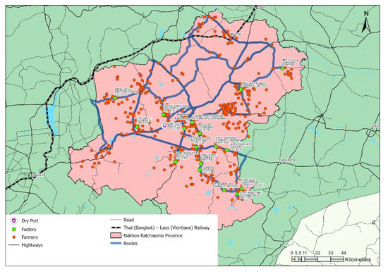
Figure 12. Example routes of the case study are assigned to 17 factories.

Figure 12 shows that the example routes in the case study were assigned to 17 factories. We noted that the budget constraints of the buy–sell price of tapioca starch and the price of oil grew. We evaluated how they would react if demand grows. The experiment was carried out on a case study by increasing the demand of 33 factories by 10%, 20%, 30%, 40%, and 50%. The computational results of the shipping cost, total cost, and profit are shown in Table 24.

Table 24. Computational results addition demand of factories in the case study.

Addition Demand of Factories (%)	Demand (tons)	Sell Cost (Bath)	MDEALNS			DE			ALNS
			Shipping Cost (Bath)	Total Cost (Bath)	Profit (Bath)	Shipping Cost (Bath)	Total Cost (Bath)	Profit (Bath)	Shipping Cost (Bath)	Total Cost (Bath)	Profit (Bath)
10%	116.00	2,474,280.00	42,742	2,431,538.00	20,961.53	44,107	2,430,173.00	20,949.77	44,562	2,429,718.00	20,945.84
20%	232.01	4,948,773.30	42,987	4,905,786.30	21,144.72	44,766	4,904,007.30	21,137.05	44,987	4,903,786.30	21,136.10
30%	348.01	7,423,053.30	43,073	7,379,980.30	21,206.23	46,323	7,376,730.30	21,196.89	46,732	7,376,321.30	21,195.72
40%	464.01	9,897,333.30	43,152	9,854,181.30	21,237.00	46,298	9,851,035.30	21,230.22	47,008	9,850,325.30	21,228.69
50%	580.02	12,371,826.60	43,329	12,328,497.60	21,255.30	47,422	12,324,404.60	21,248.24	47,612	12,324,214.60	21,247.91
Average	348.01	7,423,053.30	43,057	7,379,996.70	21,160.96	45,783	7,377,270.10	21,152.43	46,180	7,376,873.10	21,150.85

Note: selling price per ton is equal to THB 21,330.

As shown in the computational results in Table 24, when the average value of the additional demand of factories was adjusted by 10%, 20%, 30%, 40%, and 50% of the shipping cost, the total cost and profit of MDEALNS surpassed those of the other approaches, in terms of finding a better solution. The average values of the lower profits using DE, ALNS, and MDEALNS were THB 21,152.43, THB 21,150.85, and THB 21,160.96, respectively.

Figure 13 shows the average value of profit when the additional demand of the factories was adjusted by 10%, 20%, 30%, 40%, and 50%.

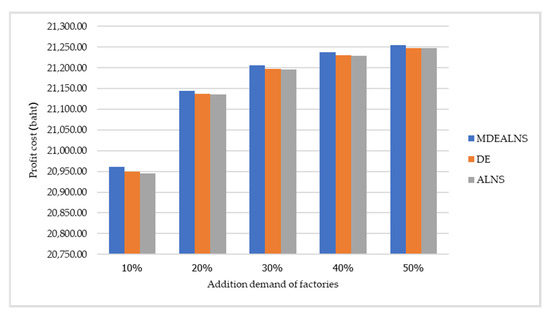
Figure 13. The value of profit with the addition demand.

5. Discussion

This research aimed to establish a tapioca starch logistics network linked to generation, along the transport route of tapioca starch products to a land port, serving as the logistics hub of Thailand’s Nakhon Ratchasima province. We presented a modified differential evolution with adaptive large neighborhood search (MDEALNS) algorithm for the minimization of distance and fuel cost. This is composed of the following six steps: (1) initialization by initial population decoding; (2) mutation; (3) recombination; (4) adaptive large neighborhood search (ALNS); (5) selection; and (6) repetition of steps 2–5 until the termination condition is met.

Three methods, i.e., MDEALNS, DE, and ALNS, were used to evaluate the performance of solving the tapioca starch logistics network problem. The datasets of the three groups of test instances and the case study consisted of 404 farms, 33 factories, and 1 land port. The computational output results showed that the MDEALNS method outperformed the DE and ALNS methods, due to it providing a better answer and taking less time to process the answer than the other methods.

MDEALNS is a new meta-heuristic concept derived from the DE method structure, which is easily understood and not complex, and the ALNS method is used to search for a solution in a large area. Therefore, the combination of the two methods generated the best answer, making this combination effective in regards to resolving problems.

The MDEALNS method outperformed the best-known previous method (LINGO v.13), finding the optimal solution of datasets for the three groups and the case study. LINGO could only find the best objective and lower bound within 7200 min, but the MDEALNS method could find the optimal solution within an average time of 2.5 min. The case study results show that the proposed MDEALNS method reduced the distance to 4101.78 km and the fuel cost to THB 42,650.56. When the constraints of the factories’ additional demands were increased by 10%, 20%, 30%, 40%, and 50%, the MDEALNS method achieved a higher profit than the DE and ALNS methods.

Future research should also study factors that are more complicated in the tapioca starch logistics network problem, such as the different types of roads used for delivery, e.g., narrow roads, which are only suitable for small cars and not for large trucks or trailers; this factor is related to delivery time. Moreover, the road type is related to the calculation of the vehicle’s energy consumption rate, by applying the principles of the methods, which may be in the form of the software or applications used to collect data, the exchange of information between organizations that use planning for logistics networks, or solutions to various problems that occur.

References

- Commission Communication, Cf. White Paper Roadmap to a Single European Transport Area–Towards a Competitive and Resource Efficient Transport System; European Commission: Brussels, Belgium, 2011. [Google Scholar]
- Mindur, L.; Wronka, J. Transport kombinowany/intermodalny. In Uwarunkowania Rozwoju Systemu Transportowego Polski; Wydawnictwo Instytutu Technologii Eksploatacji—PIB: Warszawa, Poland, 2007; pp. 349–393. [Google Scholar]
- Montwiłł, A. Inland ports in the urban logistics system. Case studies. Transp. Res. Procedia 2019, 39, 333–340. [Google Scholar] [CrossRef]
- Kurtuluş, E. Optimizing Inland Container Logistics and Dry Port Location-Allocation from an Environmental Perspective. Res. Transp. Bus. Manag. 2022, 100839. [Google Scholar] [CrossRef]
- Roso, V.; Woxenius, J.; Lumsden, K. The dry port concept: Connecting container seaports with the hinterland. J. Transp. Geogr. 2009, 17, 338–345. [Google Scholar] [CrossRef]
- Tsao, Y.-C.; Linh, V.T. Seaport-dry port network design considering multimodal transport and carbon emissions. J. Clean. Prod. 2018, 199, 481–492. [Google Scholar] [CrossRef]
- Li, W.; Hilmola, O.-P.; Panova, Y. Container sea ports and dry ports: Future CO2 emission reduction potential in China. Sustainability 2019, 11, 1515. [Google Scholar] [CrossRef]
- Kurtulus, E.; Cetin, I.B. Assessing the environmental benefits of dry port usage: A case of inland container transport in Turkey. Sustainability 2019, 11, 6793. [Google Scholar] [CrossRef]
- Lovrić, I.; Bartulović, D.; Viduka, M.; Steiner, S. Simulation analysis of seaport rijeka operations with established dry port. Pomorstvo 2020, 34, 129–145. [Google Scholar] [CrossRef]
- Liu, Y.F.; Lee, C.B.; Qi, G.Q.; Yuen, K.F.; Su, M. Relationship Between Dry Ports and Regional Economy: Evidence from Yangtze River Economic Belt. J. Asian Financ. Econ. Bus. 2021, 8, 345–354. [Google Scholar]
- Lovrić, I.; Bartulović, D.; Steiner, S. The influence of dry port establishment on regional development through regional development index. Trans. Marit. Sci. 2020, 9, 293–315. [Google Scholar] [CrossRef]
- Robinson, R. Ports as elements in value-driven chain systems: The new paradigm. Marit. Policy Manag. 2002, 29, 241–255. [Google Scholar] [CrossRef]
- Rahimi, M.; Asef-Vaziri, A.; Harrison, R. An inland port location-allocation model for a regional intermodal goods movement system. Marit. Econ. Logist. 2008, 10, 362–379. [Google Scholar] [CrossRef]
- Henttu, V.; Hilmola, O.-P. Financial and environmental impacts of hypothetical Finnish dry port structure. Res. Transp. Econ. 2011, 33, 35–41. [Google Scholar] [CrossRef]
- Nguyen, L.C.; Notteboom, T. A multi-criteria approach to dry port location in developing economies with application to Vietnam. Asian J. Shipp. Logist. 2016, 32, 23–32. [Google Scholar] [CrossRef]
- Kardung, M.; Cingiz, K.; Costenoble, O.; Delahaye, R.; Heijman, W.; Lovrić, M.; van Leeuwen, M.; M’barek, R.; van Meijl, H.; Piotrowski, S. Development of the circular bioeconomy: Drivers and indicators. Sustainability 2021, 13, 413. [Google Scholar] [CrossRef]
- Tadić, S.; Krstić, M.; Roso, V.; Brnjac, N. Dry port terminal location selection by applying the hybrid grey MCDM model. Sustainability 2020, 12, 6983. [Google Scholar] [CrossRef]
- Komchornrit, K. The selection of dry port location by a hybrid CFA-MACBETH-PROMETHEE method: A case study of Southern Thailand. Asian J. Shipp. Logist. 2017, 33, 141–153. [Google Scholar] [CrossRef]
- Monios, J.; Wilmsmeier, G. Port-centric logistics, dry ports and offshore logistics hubs: Strategies to overcome double peripherality? Marit. Policy Manag. 2012, 39, 207–226. [Google Scholar] [CrossRef]
- Ambrosino, D.; Sciomachen, A. Location of mid-range dry ports in multimodal logistic networks. Procedia-Soc. Behav. Sci. 2014, 108, 118–128. [Google Scholar] [CrossRef]
- Wang, C.; Chen, Q.; Huang, R. Locating dry ports on a network: A case study on Tianjin Port. Marit. Policy Manag. 2018, 45, 71–88. [Google Scholar] [CrossRef]
- Wei, H.; Dong, M. Import-export freight organization and optimization in the dry-port-based cross-border logistics network under the Belt and Road Initiative. Comput. Ind. Eng. 2019, 130, 472–484. [Google Scholar] [CrossRef]
- Fazi, S.; Fransoo, J.C.; Van Woensel, T.; Dong, J.-X. A variant of the split vehicle routing problem with simultaneous deliveries and pickups for inland container shipping in dry-port based systems. Transp. Res. Part E Logist. Transp. Rev. 2020, 142, 102057. [Google Scholar] [CrossRef]
- Akararungruangkul, R.; Kaewman, S. Modified differential evolution algorithm solving the special case of location routing problem. Math. Comput. Appl. 2018, 23, 34. [Google Scholar] [CrossRef]
- Yuchi, Q.; Wang, N.; He, Z.; Chen, H. Hybrid heuristic for the location-inventory-routing problem in closed-loop supply chain. Int. Trans. Oper. Res. 2018, 28, 1265–1295. [Google Scholar] [CrossRef]
- Hernández-Mejía, C.; Torres-Muñoz, D.; Inzunza-González, E.; Sánchez-López, C.; García-Guerrero, E.E. A Novel Green Logistics Technique for Planning Merchandise Deliveries: A Case Study. Logistics 2022, 6, 59. [Google Scholar] [CrossRef]
- Lo, S.-C. A Particle Swarm Optimization Approach to Solve the Vehicle Routing Problem with Cross-Docking and Carbon Emissions Reduction in Logistics Management. Logistics 2022, 6, 62. [Google Scholar] [CrossRef]
- Mehdi, N.; Abdelmoutalib, M.; Imad, H. A modified ALNS algorithm for vehicle routing problems with time windows. Proc. J. Phys. Conf. Ser. 2021, 1743, 012029. [Google Scholar] [CrossRef]
- Khamsing, N.; Chindaprasert, K.; Pitakaso, R.; Sirirak, W.; Theeraviriya, C. Modified ALNS algorithm for a processing application of family tourist route planning: A case study of Buriram in Thailand. Computation 2021, 9, 23. [Google Scholar] [CrossRef]
- Han, B.; Shi, S.; Gao, H.; Hu, Y. A Sustainable Intermodal Location-Routing Optimization Approach: A Case Study of the Bohai Rim Region. Sustainability 2022, 14, 3987. [Google Scholar] [CrossRef]
- Moonsri, K.; Sethanan, K.; Worasan, K.; Nitisiri, K. A Hybrid and Self-Adaptive Differential Evolution Algorithm for the Multi-Depot Vehicle Routing Problem in Egg Distribution. Appl. Sci. 2021, 12, 35. [Google Scholar] [CrossRef]
- Institute of Collaborative Logistics and Transportation. Available online: https://rmuti.ac.th/main/rmutinews080765-1/ (accessed on 24 July 2022).
- Pitakaso, R.; Nanthasamroeng, N.; Srichok, T.; Khonjun, S.; Weerayuth, N.; Kotmongkol, T.; Pornprasert, P.; Pranet, K. A Novel Artificial Multiple Intelligence System (AMIS) for Agricultural Product Transborder Logistics Network Design in the Greater Mekong Subregion (GMS). Computation 2022, 10, 126. [Google Scholar] [CrossRef]
- Castaneda, J.; Ghorbani, E.; Ammouriova, M.; Panadero, J.; Juan, A.A. Optimizing Transport Logistics under Uncertainty with Simheuristics: Concepts, Review and Trends. Logistics 2022, 6, 42. [Google Scholar] [CrossRef]
- Sethanan, K.; Pitakaso, R. Differential evolution algorithms for scheduling raw milk transportation. Comput. Electron. Agric. 2016, 121, 245–259. [Google Scholar] [CrossRef]
- Storn, R.; Price, K. Minimizing the real functions of the ICEC’96 contest by differential evolution. In Proceedings of the IEEE International Conference on Evolutionary Computation, Nagoya, Japan, 20–22 May 1996; pp. 842–844. [Google Scholar]
- Gämperle, R.; Müller, S.D.; Koumoutsakos, P. A parameter study for differential evolution. Adv. Intell. Syst. Fuzzy Syst. Evol. Comput. 2002, 10, 293–298. [Google Scholar]
Publisher’s Note: MDPI stays neutral with regard to jurisdictional claims in published maps and institutional affiliations. |
© 2022 by the authors. Licensee MDPI, Basel, Switzerland. This article is an open access article distributed under the terms and conditions of the Creative Commons Attribution (CC BY) license (https://creativecommons.org/licenses/by/4.0/).