
MDEALNS for Solving the Tapioca Starch Logistics Network Problem for the Land Port of Nakhon Ratchasima Province, Thailand

Abstract
1. Introduction
2. Problem Definition of NR-DP
3. Modified Differential Evolution with Adaptive Large Neighborhood Search
- (1)
- Initialization
- (2)
- Mutation
- (3)
- Recombination
- (4)
- ALNS
- (5)
- Selection
- (6)
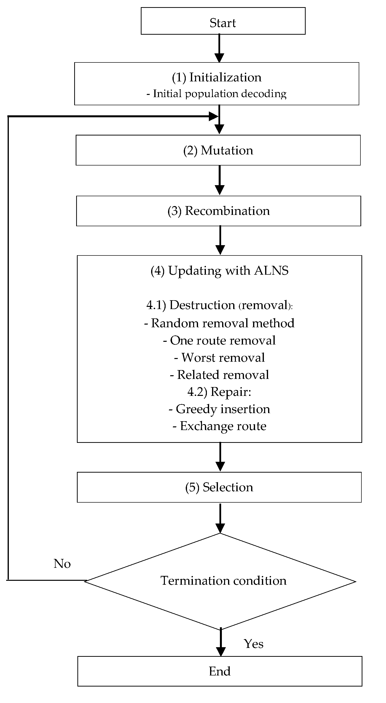
- Repeat steps 2–5 until the termination condition is met. Figure 4 shows a flowchart of MDEALNS.
3.1. Initialization
Initial Population Decoding
- (1)
- Vehicle size with a capacity of 15 tons requires the use of the lower bound of 0.01–0.50.
- (2)
- The 30-ton vehicles are required to use the upper bound of 0.51–1.00.
3.2. Mutation
3.3. Recombination
3.4. Adaptive Large Neighborhood Search (ALNS)
| Algorithm 1: Algorithm of Adaptive Large Neighborhood Search |
| Input: problem instance I |
| create initial solution Smin = S ∈ S(I) |
| while stopping criteria not met do |
| for i = 1,…, pu do |
| select r ∈ R, d ∈ D according to probabilities p |
| S′ = r(d(S)) |
| if accept(S, S′) then |
| S = S′ |
| if c(S) < c(Smin) then |
| Smin = S |
| adjust the value of the current solution |
| Return smin |
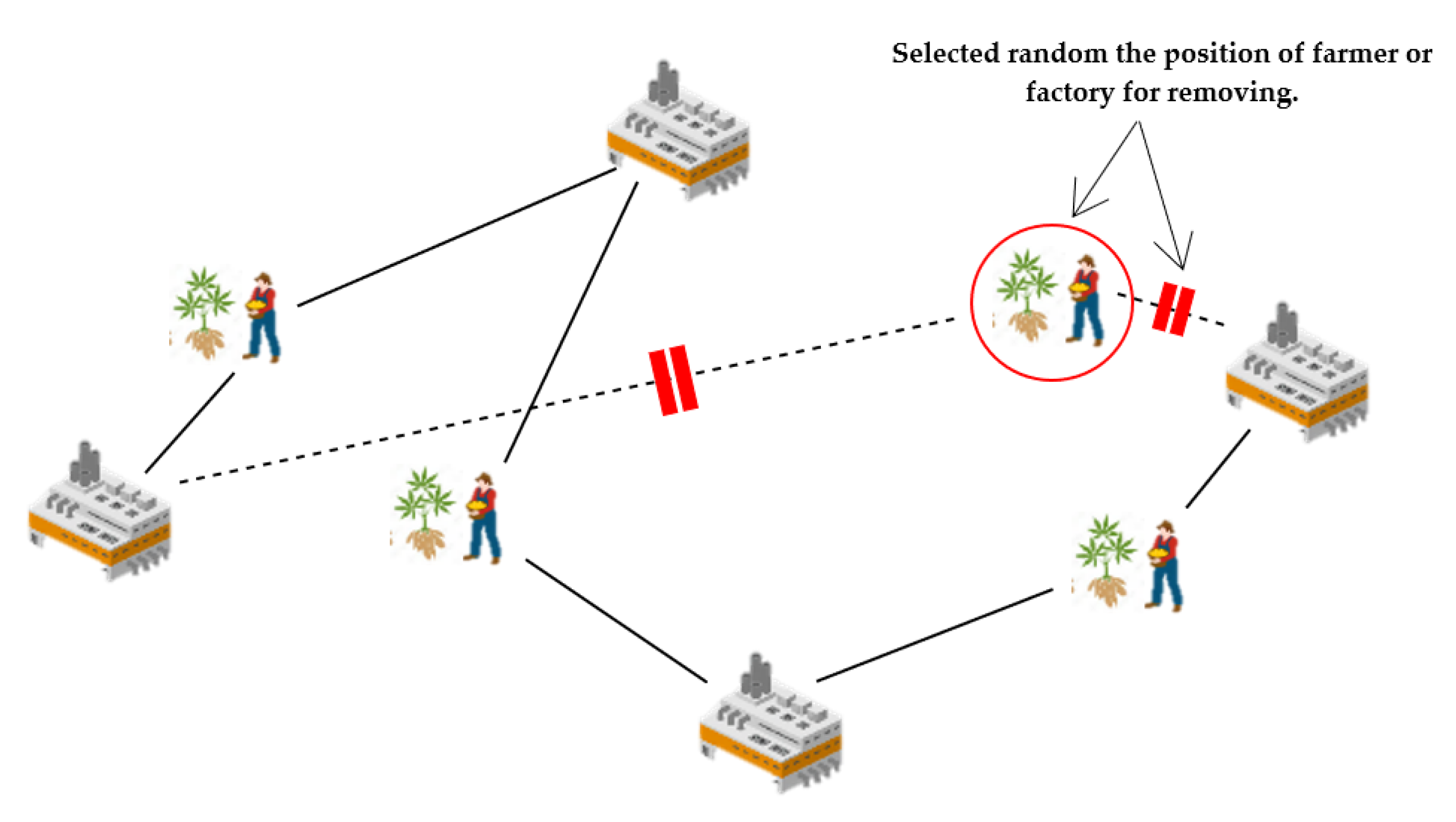
- (1)
- The random removal method is used to randomly select the position of the farmer or the position of the factory on the exit route, in order to rearrange the route, resulting in a pattern that destroys the answer, as shown in Figure 5.
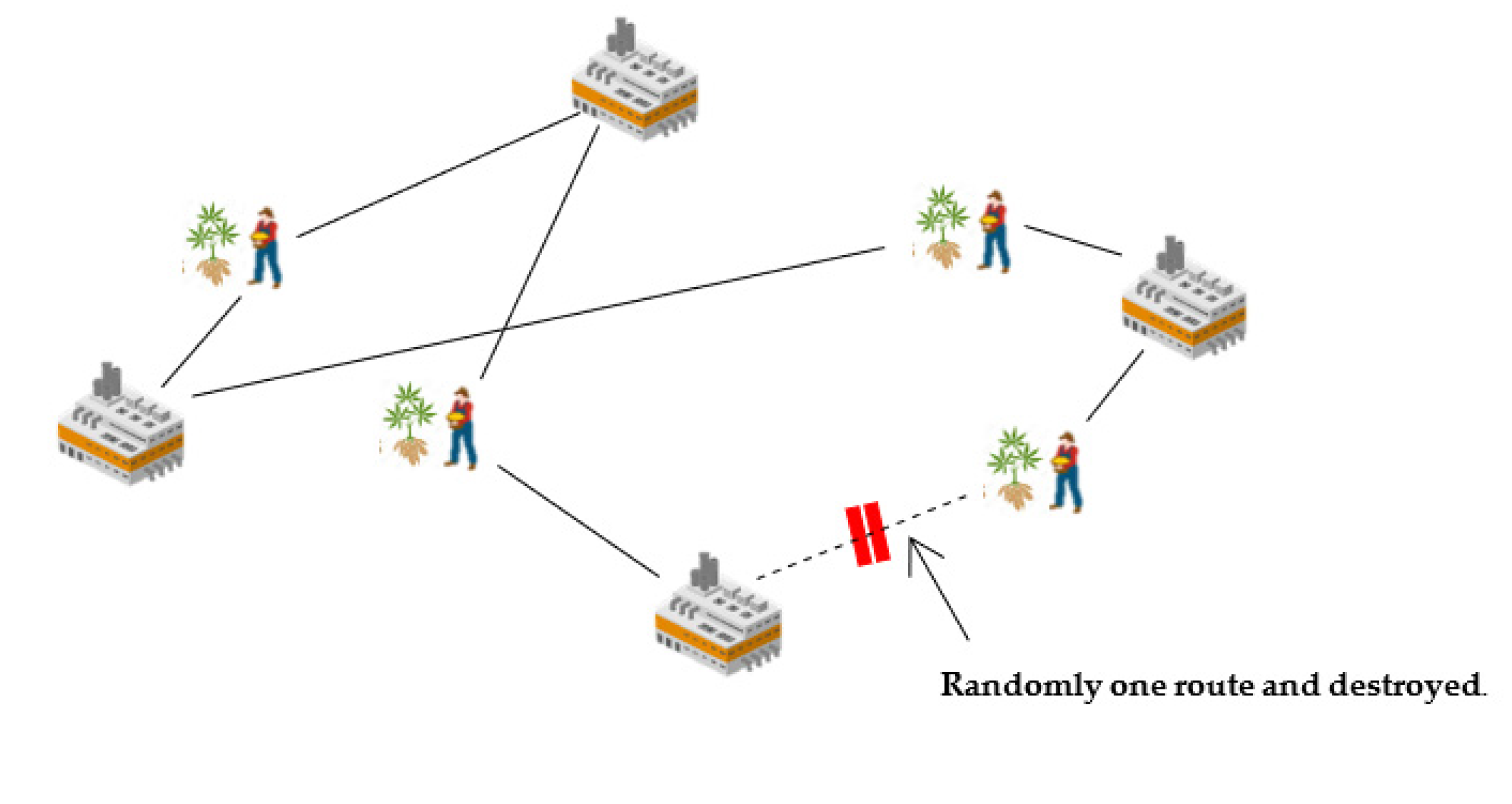
- (2)
- One route removal is the random destruction of a route that is separate from all the other routes, resulting in a pattern that destroys the answer, as shown in Figure 6.
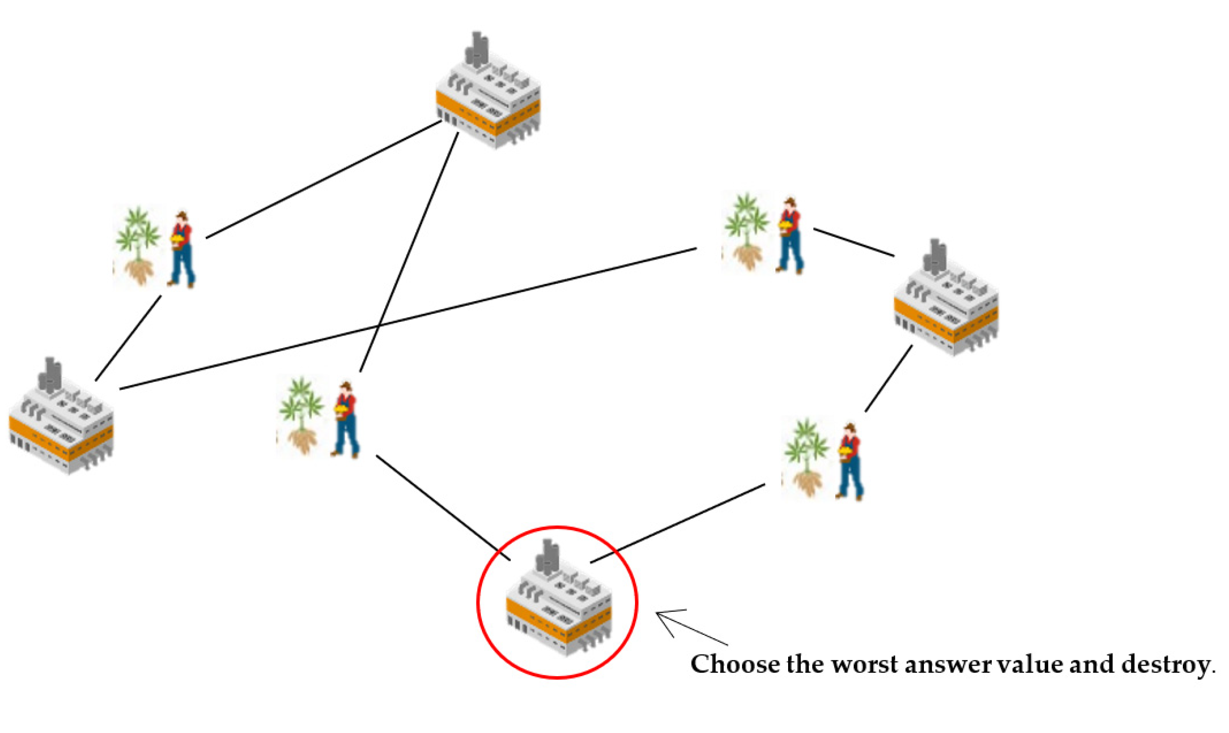
- (3)
- Worst removal destroys the answer resulting from the worst answer of the farmer or destroys the worst answer of the factory, resulting in a pattern that destroys the answer, as shown in Figure 7.
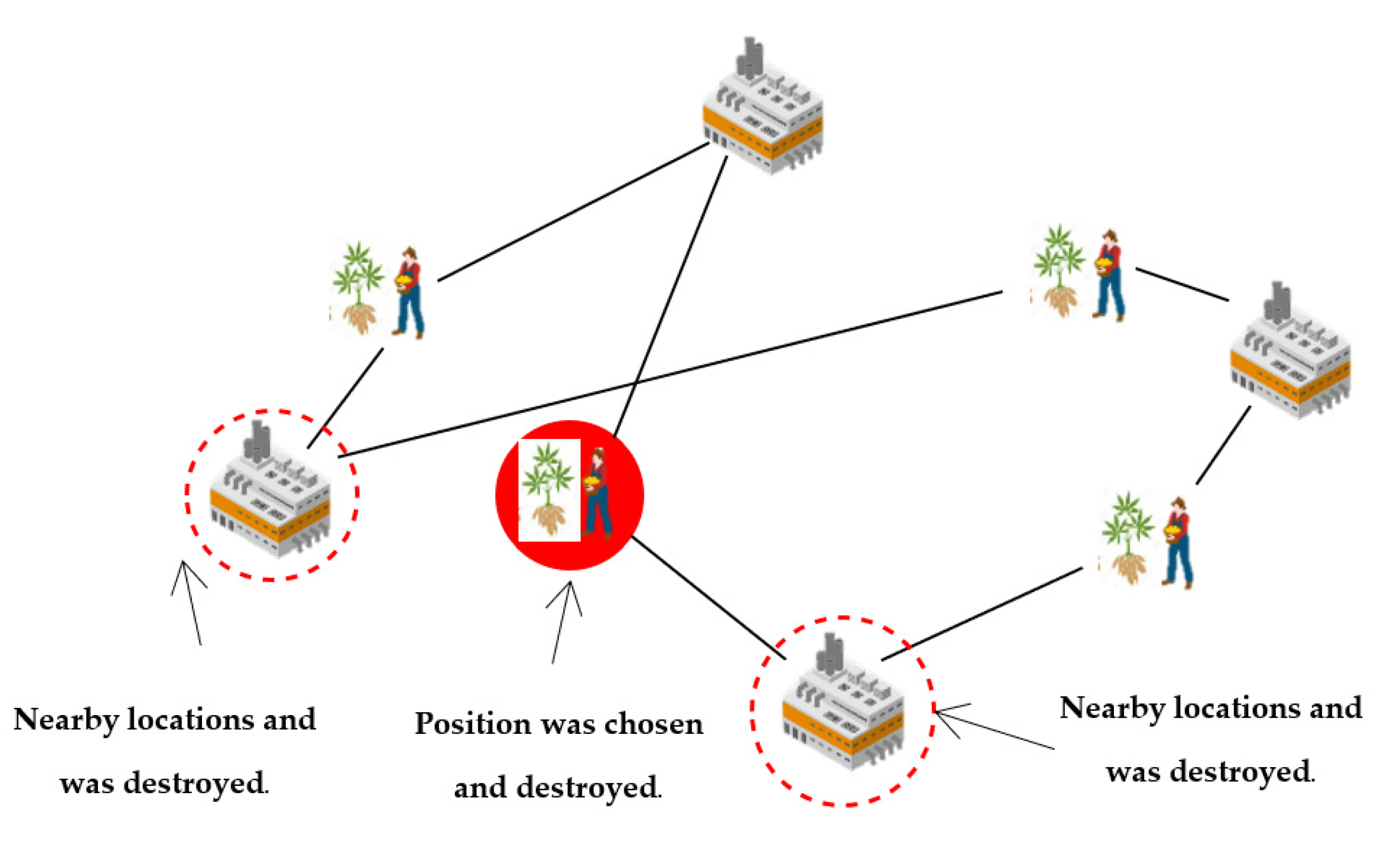
- (4)
- Related removal destroys the answer based on the neighboring position relative to the chosen position being destroyed, resulting in a pattern that destroys the answer, as shown in Figure 8.
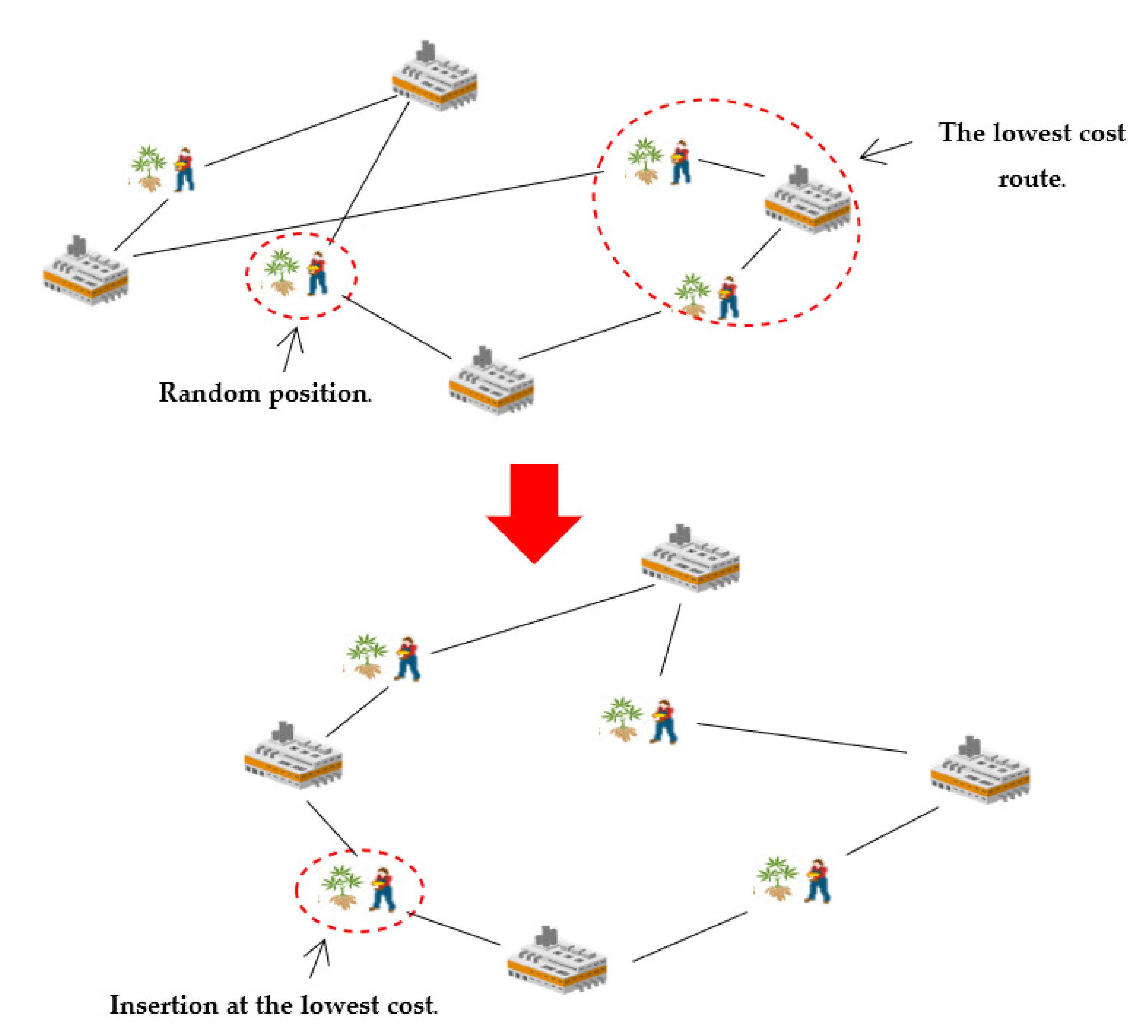
- (1)
- Greedy insertion is a method of repairing the answer by taking the difference with the lowest total distance and inserting it again, which results in a new answer, as shown in Figure 9.
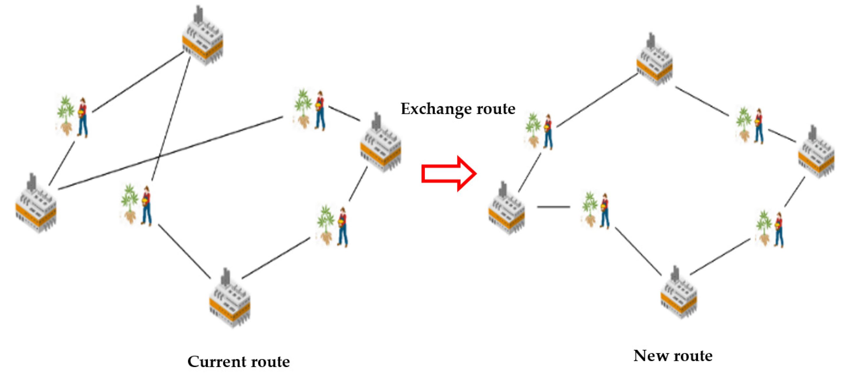
- (2)
- An exchange route is an answer repair method, which swaps the entire route for a new, lower cost route by randomly selecting a path for destruction. Once that path is removed, a new path is created, improving and, thus, repairing the answer, as shown in Figure 10.
3.5. Selection
3.6. Repeating
4. Computational Results
Datasets for Solving the Tapioca Starch Logistics Network Problem
5. Discussion
Author Contributions
Funding
Data Availability Statement
Acknowledgments
Conflicts of Interest
References
- Commission Communication, Cf. White Paper Roadmap to a Single European Transport Area–Towards a Competitive and Resource Efficient Transport System; European Commission: Brussels, Belgium, 2011. [Google Scholar]
- Mindur, L.; Wronka, J. Transport kombinowany/intermodalny. In Uwarunkowania Rozwoju Systemu Transportowego Polski; Wydawnictwo Instytutu Technologii Eksploatacji—PIB: Warszawa, Poland, 2007; pp. 349–393. [Google Scholar]
- Montwiłł, A. Inland ports in the urban logistics system. Case studies. Transp. Res. Procedia 2019, 39, 333–340. [Google Scholar] [CrossRef]
- Kurtuluş, E. Optimizing Inland Container Logistics and Dry Port Location-Allocation from an Environmental Perspective. Res. Transp. Bus. Manag. 2022, 100839. [Google Scholar] [CrossRef]
- Roso, V.; Woxenius, J.; Lumsden, K. The dry port concept: Connecting container seaports with the hinterland. J. Transp. Geogr. 2009, 17, 338–345. [Google Scholar] [CrossRef]
- Tsao, Y.-C.; Linh, V.T. Seaport-dry port network design considering multimodal transport and carbon emissions. J. Clean. Prod. 2018, 199, 481–492. [Google Scholar] [CrossRef]
- Li, W.; Hilmola, O.-P.; Panova, Y. Container sea ports and dry ports: Future CO2 emission reduction potential in China. Sustainability 2019, 11, 1515. [Google Scholar] [CrossRef]
- Kurtulus, E.; Cetin, I.B. Assessing the environmental benefits of dry port usage: A case of inland container transport in Turkey. Sustainability 2019, 11, 6793. [Google Scholar] [CrossRef]
- Lovrić, I.; Bartulović, D.; Viduka, M.; Steiner, S. Simulation analysis of seaport rijeka operations with established dry port. Pomorstvo 2020, 34, 129–145. [Google Scholar] [CrossRef]
- Liu, Y.F.; Lee, C.B.; Qi, G.Q.; Yuen, K.F.; Su, M. Relationship Between Dry Ports and Regional Economy: Evidence from Yangtze River Economic Belt. J. Asian Financ. Econ. Bus. 2021, 8, 345–354. [Google Scholar]
- Lovrić, I.; Bartulović, D.; Steiner, S. The influence of dry port establishment on regional development through regional development index. Trans. Marit. Sci. 2020, 9, 293–315. [Google Scholar] [CrossRef]
- Robinson, R. Ports as elements in value-driven chain systems: The new paradigm. Marit. Policy Manag. 2002, 29, 241–255. [Google Scholar] [CrossRef]
- Rahimi, M.; Asef-Vaziri, A.; Harrison, R. An inland port location-allocation model for a regional intermodal goods movement system. Marit. Econ. Logist. 2008, 10, 362–379. [Google Scholar] [CrossRef]
- Henttu, V.; Hilmola, O.-P. Financial and environmental impacts of hypothetical Finnish dry port structure. Res. Transp. Econ. 2011, 33, 35–41. [Google Scholar] [CrossRef]
- Nguyen, L.C.; Notteboom, T. A multi-criteria approach to dry port location in developing economies with application to Vietnam. Asian J. Shipp. Logist. 2016, 32, 23–32. [Google Scholar] [CrossRef]
- Kardung, M.; Cingiz, K.; Costenoble, O.; Delahaye, R.; Heijman, W.; Lovrić, M.; van Leeuwen, M.; M’barek, R.; van Meijl, H.; Piotrowski, S. Development of the circular bioeconomy: Drivers and indicators. Sustainability 2021, 13, 413. [Google Scholar] [CrossRef]
- Tadić, S.; Krstić, M.; Roso, V.; Brnjac, N. Dry port terminal location selection by applying the hybrid grey MCDM model. Sustainability 2020, 12, 6983. [Google Scholar] [CrossRef]
- Komchornrit, K. The selection of dry port location by a hybrid CFA-MACBETH-PROMETHEE method: A case study of Southern Thailand. Asian J. Shipp. Logist. 2017, 33, 141–153. [Google Scholar] [CrossRef]
- Monios, J.; Wilmsmeier, G. Port-centric logistics, dry ports and offshore logistics hubs: Strategies to overcome double peripherality? Marit. Policy Manag. 2012, 39, 207–226. [Google Scholar] [CrossRef]
- Ambrosino, D.; Sciomachen, A. Location of mid-range dry ports in multimodal logistic networks. Procedia-Soc. Behav. Sci. 2014, 108, 118–128. [Google Scholar] [CrossRef]
- Wang, C.; Chen, Q.; Huang, R. Locating dry ports on a network: A case study on Tianjin Port. Marit. Policy Manag. 2018, 45, 71–88. [Google Scholar] [CrossRef]
- Wei, H.; Dong, M. Import-export freight organization and optimization in the dry-port-based cross-border logistics network under the Belt and Road Initiative. Comput. Ind. Eng. 2019, 130, 472–484. [Google Scholar] [CrossRef]
- Fazi, S.; Fransoo, J.C.; Van Woensel, T.; Dong, J.-X. A variant of the split vehicle routing problem with simultaneous deliveries and pickups for inland container shipping in dry-port based systems. Transp. Res. Part E Logist. Transp. Rev. 2020, 142, 102057. [Google Scholar] [CrossRef]
- Akararungruangkul, R.; Kaewman, S. Modified differential evolution algorithm solving the special case of location routing problem. Math. Comput. Appl. 2018, 23, 34. [Google Scholar] [CrossRef]
- Yuchi, Q.; Wang, N.; He, Z.; Chen, H. Hybrid heuristic for the location-inventory-routing problem in closed-loop supply chain. Int. Trans. Oper. Res. 2018, 28, 1265–1295. [Google Scholar] [CrossRef]
- Hernández-Mejía, C.; Torres-Muñoz, D.; Inzunza-González, E.; Sánchez-López, C.; García-Guerrero, E.E. A Novel Green Logistics Technique for Planning Merchandise Deliveries: A Case Study. Logistics 2022, 6, 59. [Google Scholar] [CrossRef]
- Lo, S.-C. A Particle Swarm Optimization Approach to Solve the Vehicle Routing Problem with Cross-Docking and Carbon Emissions Reduction in Logistics Management. Logistics 2022, 6, 62. [Google Scholar] [CrossRef]
- Mehdi, N.; Abdelmoutalib, M.; Imad, H. A modified ALNS algorithm for vehicle routing problems with time windows. Proc. J. Phys. Conf. Ser. 2021, 1743, 012029. [Google Scholar] [CrossRef]
- Khamsing, N.; Chindaprasert, K.; Pitakaso, R.; Sirirak, W.; Theeraviriya, C. Modified ALNS algorithm for a processing application of family tourist route planning: A case study of Buriram in Thailand. Computation 2021, 9, 23. [Google Scholar] [CrossRef]
- Han, B.; Shi, S.; Gao, H.; Hu, Y. A Sustainable Intermodal Location-Routing Optimization Approach: A Case Study of the Bohai Rim Region. Sustainability 2022, 14, 3987. [Google Scholar] [CrossRef]
- Moonsri, K.; Sethanan, K.; Worasan, K.; Nitisiri, K. A Hybrid and Self-Adaptive Differential Evolution Algorithm for the Multi-Depot Vehicle Routing Problem in Egg Distribution. Appl. Sci. 2021, 12, 35. [Google Scholar] [CrossRef]
- Institute of Collaborative Logistics and Transportation. Available online: https://rmuti.ac.th/main/rmutinews080765-1/ (accessed on 24 July 2022).
- Pitakaso, R.; Nanthasamroeng, N.; Srichok, T.; Khonjun, S.; Weerayuth, N.; Kotmongkol, T.; Pornprasert, P.; Pranet, K. A Novel Artificial Multiple Intelligence System (AMIS) for Agricultural Product Transborder Logistics Network Design in the Greater Mekong Subregion (GMS). Computation 2022, 10, 126. [Google Scholar] [CrossRef]
- Castaneda, J.; Ghorbani, E.; Ammouriova, M.; Panadero, J.; Juan, A.A. Optimizing Transport Logistics under Uncertainty with Simheuristics: Concepts, Review and Trends. Logistics 2022, 6, 42. [Google Scholar] [CrossRef]
- Sethanan, K.; Pitakaso, R. Differential evolution algorithms for scheduling raw milk transportation. Comput. Electron. Agric. 2016, 121, 245–259. [Google Scholar] [CrossRef]
- Storn, R.; Price, K. Minimizing the real functions of the ICEC’96 contest by differential evolution. In Proceedings of the IEEE International Conference on Evolutionary Computation, Nagoya, Japan, 20–22 May 1996; pp. 842–844. [Google Scholar]
- Gämperle, R.; Müller, S.D.; Koumoutsakos, P. A parameter study for differential evolution. Adv. Intell. Syst. Fuzzy Syst. Evol. Comput. 2002, 10, 293–298. [Google Scholar]


| Farmer | |||||
|---|---|---|---|---|---|
| Factory | 1 | 2 | 3 | 4 | 5 |
| 1 | 0.23 | 0.72 | 0.31 | 0.68 | 0.17 |
| 2 | 0.47 | 0.48 | 0.41 | 0.06 | 0.67 |
| 3 | 0.86 | 0.49 | 0.71 | 0.82 | 0.83 |
| Factory | 1 | 2 | 3 | ||
| Demand (tons) | 30 | 40 | 35 | ||
| Farmer | 1 | 2 | 3 | 4 | 5 |
| Production capacity (tons) | 15 | 27 | 28 | 20 | 15 |
| Capacity = 15 tons and 30 tons | Fuel cost = 35 baht/L | ||||
| Farmer | |||||
|---|---|---|---|---|---|
| 1 | 2 | 3 | 4 | 5 | |
| Factory | 0.23 | 0.72 | 0.31 | 0.68 | 0.17 |
| Farmer | |||||
|---|---|---|---|---|---|
| 5 | 1 | 3 | 4 | 2 | |
| Factory | 0.17 | 0.23 | 0.31 | 0.68 | 0.72 |
| Factory | Farmer | ||||||||
|---|---|---|---|---|---|---|---|---|---|
| 1 | 2 | 3 | 1 | 2 | 3 | 4 | 5 | ||
| Factory | 1 | - | 3 | 16 | 20 | 36 | 45 | 78 | 90 |
| 2 | 3 | - | 18 | 37 | 41 | 87 | 98 | 103 | |
| 3 | 16 | 18 | - | 66 | 82 | 107 | 111 | 124 | |
| Farmer | 1 | 20 | 37 | 66 | - | 98 | 121 | 132 | 144 |
| 2 | 36 | 41 | 82 | 98 | - | 108 | 122 | 167 | |
| 3 | 45 | 87 | 107 | 121 | 108 | - | 98 | 135 | |
| 4 | 78 | 98 | 111 | 132 | 122 | 98 | - | 153 | |
| 5 | 90 | 103 | 124 | 144 | 167 | 135 | 153 | - | |
| Factory | Farmer | ||||||||
|---|---|---|---|---|---|---|---|---|---|
| 1 | 2 | 3 | 1 | 2 | 3 | 4 | 5 | ||
| Factory | 1 | - | 15 tons | 15 tons | 30 tons | 30 tons | 15 tons | 15 tons | 15 tons |
| 2 | 15 tons | - | 30 tons | 30 tons | 30 tons | 30 tons | 15 tons | 15 tons | |
| 3 | 15 tons | 30 tons | - | 15 tons | 30 tons | 30 tons | 30 tons | 15 tons | |
| Farmer | 1 | 30 tons | 30 tons | 15 tons | - | 30 tons | 15 tons | 15 tons | 30 tons |
| 2 | 30 tons | 30 tons | 30 tons | 30 tons | - | 15 tons | 30 tons | 30 tons | |
| 3 | 15 tons | 30 tons | 30 tons | 15 tons | 15 tons | - | 15 tons | 15 tons | |
| 4 | 15 tons | 15 tons | 30 tons | 15 tons | 30 tons | 15 tons | - | 30 tons | |
| 5 | 15 tons | 15 tons | 15 tons | 30 tons | 30 tons | 15 tons | 30 tons | - | |
| No. | Route | Distance (km) | Capacity of Car (tons) | Fuel Consumption Rate (km/L) | Cost of Fuel (Baht) |
|---|---|---|---|---|---|
| 1 | Farmer 5-Factory 1 | 90 | 15 | 3 | 1050.00 |
| Farmer 1-Factory 1 | 20 | 30 | 4 | 175.00 | |
| 2 | Farmer 3-Factory 2 | 87 | 30 | 4 | 761.25 |
| Farmer 4-Factory 2 | 98 | 15 | 3 | 1143.33 | |
| 3 | Factory 4-Farmer 2 | 122 | 30 | 4 | 1067.50 |
| Farmer 2-Factory 3 | 82 | 30 | 4 | 717.50 | |
| Factory 3-Farmer 2 | 82 | 30 | 4 | 717.50 | |
| Farmer 2-Factory 3 | 82 | 30 | 4 | 717.50 | |
| Total of objective values. | 663 | 6349.58 | |||
| Farmer | |||||
|---|---|---|---|---|---|
| 1 | 2 | 3 | 4 | 5 | |
| Factory 1 (Target vector (Xi,G+1)) | 0.23 | 0.72 | 0.31 | 0.68 | 0.17 |
| Factory 2 (Target vector (Xi,G+1)) | 0.47 | 0.48 | 0.41 | 0.06 | 0.67 |
| Factory (Mutant vector (Vi,G+1)) | 0.26 | 0.41 | 0.76 | 0.04 | 0.66 |
| Factory | Farmer | ||||
|---|---|---|---|---|---|
| 1 | 2 | 3 | 4 | 5 | |
| Target vector random | 0.03 | 0.63 | 0.97 | 0.32 | 0.39 |
| Target vector (Xi,G+1) | 0.23 | 0.72 | 0.31 | 0.68 | 0.17 |
| Mutant vector (Vi,G+1) | 0.26 | 0.41 | 0.76 | 0.04 | 0.66 |
| Trial vector (Ui,G) | 0.26 | 0.41 | 0.31 | 0.04 | 0.66 |
| Farmer | |||||
|---|---|---|---|---|---|
| 4 | 1 | 3 | 2 | 5 | |
| Trial vector (Ui,G) | 0.04 | 0.26 | 0.31 | 0.41 | 0.66 |
| No. | Route | Distance (km) | Capacity of Car (tons) | Fuel Consumption Rate (km/L) | Cost of Fuel (Baht) |
|---|---|---|---|---|---|
| 1 | Farmer 4-Factory 1 | 78 | 15 | 3 | 910.00 |
| Farmer 4-Factory 1 | 132 | 30 | 4 | 1155.00 | |
| Farmer 1-Factory 1 | 20 | 30 | 4 | 175.00 | |
| 2 | Farmer 1-Farmer 3 | 121 | 15 | 3 | 1411.67 |
| Farmer 1-Factory 2 | 37 | 15 | 3 | 431.67 | |
| Farmer 3-Farmer 2 | 108 | 30 | 4 | 945.00 | |
| Farmer 2-Factory 2 | 41 | 30 | 4 | 358.75 | |
| 3 | Farmer 2-Factory 3 | 82 | 30 | 4 | 717.50 |
| Farmer 5-Factory 3 | 124 | 15 | 3 | 1446.67 | |
| Total of objective values. | 743 | 7551.26 | |||
| Farmer | |||||
|---|---|---|---|---|---|
| 4 | 1 | 3 | 2 | 5 | |
| Factory | 0.04 | 0.26 | 0.31 | 0.41 | 0.66 |
| Farmer | |||||
|---|---|---|---|---|---|
| 2 | 1 | 3 | 5 | 4 | |
| Factory (Trial vector) (Ui,G) | 0.41 | 0.26 | 0.31 | 0.66 | 0.04 |
| No. | Route | Distance (km) | Capacity of Car (tons) | Fuel Consumption Rate (km/L) | Cost of Fuel (Baht) |
|---|---|---|---|---|---|
| 1 | Farmer 2-Farmer 1 | 98 | 30 | 4 | 857.50 |
| Farmer 1-Factory 1 | 20 | 30 | 4 | 175.00 | |
| 2 | Farmer 1-Factory 2 | 37 | 30 | 4 | 323.75 |
| Farmer 3-Factory 2 | 87 | 30 | 4 | 761.25 | |
| 3 | Farmer 5-Factory 3 | 124 | 15 | 3 | 1446.67 |
| Farmer 4-Factory 3 | 111 | 30 | 4 | 1295.00 | |
| Total of objective values. | 477 | 4859.17 | |||
| Farmer | |||||
|---|---|---|---|---|---|
| 5 | 1 | 3 | 4 | 2 | |
| Factory (Target vector (Xi,G)) | 0.17 | 0.23 | 0.31 | 0.68 | 0.72 |
| Farmer | |||||
|---|---|---|---|---|---|
| 2 | 1 | 3 | 5 | 4 | |
| Factory (Trial vector (Ui,G)) | 0.41 | 0.26 | 0.31 | 0.66 | 0.04 |
| Instance | Farmer | Factory | Instance | Farmer | Factory |
|---|---|---|---|---|---|
| S1 | 5 | 2 | M4 | 15 | 4 |
| S2 | 6 | 2 | M5 | 15 | 4 |
| S3 | 7 | 2 | L1 | 20 | 6 |
| S4 | 8 | 3 | L2 | 40 | 7 |
| S5 | 9 | 3 | L3 | 80 | 8 |
| M1 | 10 | 4 | L4 | 150 | 10 |
| M2 | 10 | 4 | L5 | 200 | 20 |
| M3 | 15 | 4 | Case study | 404 | 33 |
| Algorithm | Definition of the Proposed Algorithms |
|---|---|
| DE | Differential Evolution |
| ALNS | Adaptive Large Neighborhood Search |
| MDEALNS | Modify Differential Evolution with Adaptive Large Neighborhood Search |
| Instance | Lingo | Status | MDEALNS | DE | ALNS | ||||||||
|---|---|---|---|---|---|---|---|---|---|---|---|---|---|
| Distance (km.) | Fuel Cost (bath) | Time (min) | Distance (km.) | Fuel Cost (bath) | Time (min) | Distance (km.) | Fuel Cost (bath) | Time (min) | Distance (km.) | Fuel Cost (bath) | Time (min) | ||
| S1 | 35.6 | 415.3 | 0.06 | Glo.opt | 35.6 | 415.3 | 0.04 | 35.6 | 415.3 | 0.05 | 35.6 | 415.3 | 0.05 |
| S2 | 57.8 | 674.3 | 0.15 | Glo.opt | 57.8 | 674.3 | 0.04 | 57.8 | 674.3 | 0.09 | 57.8 | 674.3 | 0.09 |
| S3 | 76.3 | 890.2 | 0.05 | Glo.opt | 76.3 | 890.2 | 0.04 | 76.3 | 890.2 | 0.04 | 76.3 | 890.2 | 0.04 |
| S4 | 88.7 | 1034.8 | 0.1 | Glo.opt | 88.7 | 1034.8 | 0.05 | 88.7 | 1034.8 | 0.06 | 88.7 | 1034.8 | 0.06 |
| S5 | 126 | 1102.5 | 0.09 | Glo.opt | 126 | 1102.5 | 0.04 | 126 | 1102.5 | 0.08 | 126 | 1102.5 | 0.08 |
| M1 | 187.9 | 1644.1 | 0.55 | Glo.opt | 187.9 | 1644.1 | 0.04 | 187.9 | 1644.1 | 0.15 | 187.9 | 1644.1 | 0.17 |
| M2 | 218.4 | 1911 | 0.33 | Glo.opt | 218.4 | 1911 | 0.04 | 218.4 | 1911 | 0.18 | 218.4 | 1911 | 0.16 |
| M3 | 285.3 | 3296.4 | 0.6 | Boj * | 258.6 | 1313.4 | 0.25 | 277.2 | 2925.5 | 0.55 | 279.4 | 3004.8 | 0.58 |
| M4 | 293.1 | 3419.5 | 0.68 | Boj * | 278.3 | 1737.3 | 0.81 | 298.7 | 3213.6 | 0.67 | 305.6 | 3865.3 | 0.67 |
| M5 | 333.7 | 4546.3 | 4320 | Boj * | 302.8 | 3219.9 | 0.73 | 330.4 | 4246.3 | 2.01 | 323.8 | 4022 | 1.87 |
| L1 | 329.5 | 2883.1 | 7200 | Lower Bound | 308.2 | 1984.3 | 3.02 | 321.4 | 2782.3 | 9.67 | 320.1 | 2850.9 | 13.03 |
| L2 | 734.2 | 6788.9 | 7200 | Lower Bound | 643.4 | 6029.5 | 6.13 | 975.9 | 6539.6 | 14.03 | 992.5 | 6689.5 | 16.53 |
| L3 | 1067.1 | 10,208.4 | 7200 | Lower Bound | 843.4 | 9621.5 | 8.91 | 1115.9 | 10,721.3 | 15.71 | 1134.9 | 11,358.2 | 17.14 |
| L4 | 2532.2 | 21,242.7 | 7200 | Lower Bound | 1275.8 | 16,040.5 | 10.23 | 1485.6 | 17,908.6 | 17.42 | 1572.8 | 19,389.3 | 19.81 |
| L5 | 3644.1 | 31,583.2 | 7200 | Lower Bound | 2161.3 | 15,160.5 | 11.05 | 2665.9 | 24,081.6 | 22.16 | 2840.8 | 26,639.4 | 25.43 |
| Case study | 5221.34 | 53,301.18 | 7200 | Lower Bound | 4101.78 | 42,650.56 | 12.23 | 4948.18 | 50,512.67 | 26.32 | 5012.38 | 51,168.05 | 31.98 |
| Average | 2970.2 | 3.4 | 6.8 | 8.0 | |||||||||
| MDEALNS | DE | ALNS | |
|---|---|---|---|
| LINGO | 0.055 | 0.180 | 0.211 |
| MDEALNS | - | 0.036 | 0.033 |
| DE | - | - | 0.079 |
| MDEALNS | DE | ALNS | |
|---|---|---|---|
| LINGO | 0.050 | 0.101 | 0.164 |
| MDEALNS | - | 0.037 | 0.033 |
| DE | - | - | 0.053 |
| MDEALNS | DE | ALNS | |
|---|---|---|---|
| LINGO | 0.004 | 0.004 | 0.004 |
| MDEALNS | - | 0.010 | 0.012 |
| DE | - | - | 0.019 |
| Route | Farmer | Factory | Capacity (tons) | Distance (km) | Fuel Cost (Bath) |
|---|---|---|---|---|---|
| 1 | 1,2,3,4,5,6,7,8,9,10,11,12,13,14,15,16,17,18, 19,20,22,127,132,133,135,136,139,163,225, 226,403,404 | 1 | 15 | 341.76 | 2990.4 |
| 2 | 28,29,30,33,34,35,36,37,39,40,41,42,43,44, 45,46,49 | 2 | 30 | 157.72 | 1380.05 |
| 3 | 115,117,118,119,120,121,122,123,124,166, 178,233,234 | 3 | 30 | 174.51 | 1526.963 |
| 4 | 125,126,128,129,131,134,137,138,140,141, 142,143,144,145,146,147,148,149,150,151, 153,154,281 | 4 | 15 | 362.93 | 3175.638 |
| 5 | 130,152 | 5 | 30 | 58.34 | 510.475 |
| 6 | 155,156,157,161,162,277,314,315,316,317 | 6 | 30 | 96.51 | 844.4625 |
| 7 | 158,159,160 | 7 | 15 | 21.5 | 250.8333 |
| 8 | 179,180,181,182,183,184,186,187,188,189, 190,191,192,193,194,195,196,197,198,199, 200,201,202,203,204,205,206,207 | 8 | 15 | 135.19 | 1182.913 |
| 9 | 24,25,26,27,52,53,54,55,56,58,59,60,61,62, 64,65,67,68,70,71,72,73,74,75,77,78,79,80, 81,82,84,85,86,87,88,89,90,91,93,94,96,109, 110,164,165,167,168,169,170,171,172,173, 174,175,177,229,230,231,250,252,254,256, 368,369,372,373,374,375,386,401 | 9 | 30 | 588.82 | 5152.175 |
| 10 | 267,268,269 | 10 | 15 | 21.56 | 251.5333 |
| 11 | 275,279,280,283,285,286 | 11 | 15 | 69.76 | 813.8667 |
| 12 | 208,209,210,211,212,213,214,216,217,218, 219,221,222,223,261 | 12 | 15 | 238.97 | 2090.988 |
| 13 | 98,99,100,101,111,112,291,295,296,297, 298,299 | 13 | 15 | 80.75 | 942.0833 |
| 14 | 303,361,362,364,365 | 14 | 15 | 104 | 910 |
| 15 | 102,103,104,105,106,107,108,113,114,292,’ 293,294 | 15 | 15 | 88.23 | 1029.35 |
| 16 | 300,301,302 | 16 | 15 | 28.71 | 334.95 |
| 17 | 21,185,227,318,319,320,324,332,333,334, 335,338,339 | 17 | 30 | 157.72 | 1380.05 |
| 18 | 344,347 | 18 | 30 | 21.24 | 185.85 |
| 19 | 63,95,330,342,333,389 | 19 | 30 | 64.02 | 560.175 |
| 20 | 31,32,38,47,48,50,51,345 | 20 | 30 | 115.02 | 1006.425 |
| 21 | 349,350,351,352,356,357 | 21 | 15 | 32.03 | 373.6833 |
| 22 | 358,359,363,366 | 22 | 30 | 56.77 | 496.7375 |
| 23 | 346,348,353,355,360 | 23 | 30 | 23.1 | 202.125 |
| 24 | 377,378,384,385,391,392 | 24 | 30 | 23.08 | 201.95 |
| 25 | 57,69,76,92,116,176,232,235,236,237,238, 239,240,241,242,243,244,245,246,247,248 249,251,253,255,305,306,307,308,310,311 312,367,370,371,402 | 25 | 30 | 429.21 | 3755.588 |
| 26 | 266,270,271,272,273,274 | 26 | 15 | 41.4 | 483 |
| 27 | 258,259,260,262,263,278,282,287,290 | 27 | 15 | 57.55 | 671.4167 |
| 28 | 265,276,284 | 28 | 15 | 48.76 | 426.65 |
| 29 | 215,220,224 | 29 | 30 | 157.1 | 1374.625 |
| 30 | 288,322,323,326,328,329,337,340 | 30 | 15 | 33.2 | 387.3333 |
| 31 | 313,325 | 31 | 30 | 148.46 | 1299.025 |
| 32 | 321,327,379,380,381,382,383,388,393,394 395,396,397,398 | 32 | 15 | 55.34 | 484.225 |
| 33 | 66,336,341,386,387,390,399,400 | 33 | 15 | 68.52 | 599.55 |
| Average | 4101.78 | 42,650.56 | |||
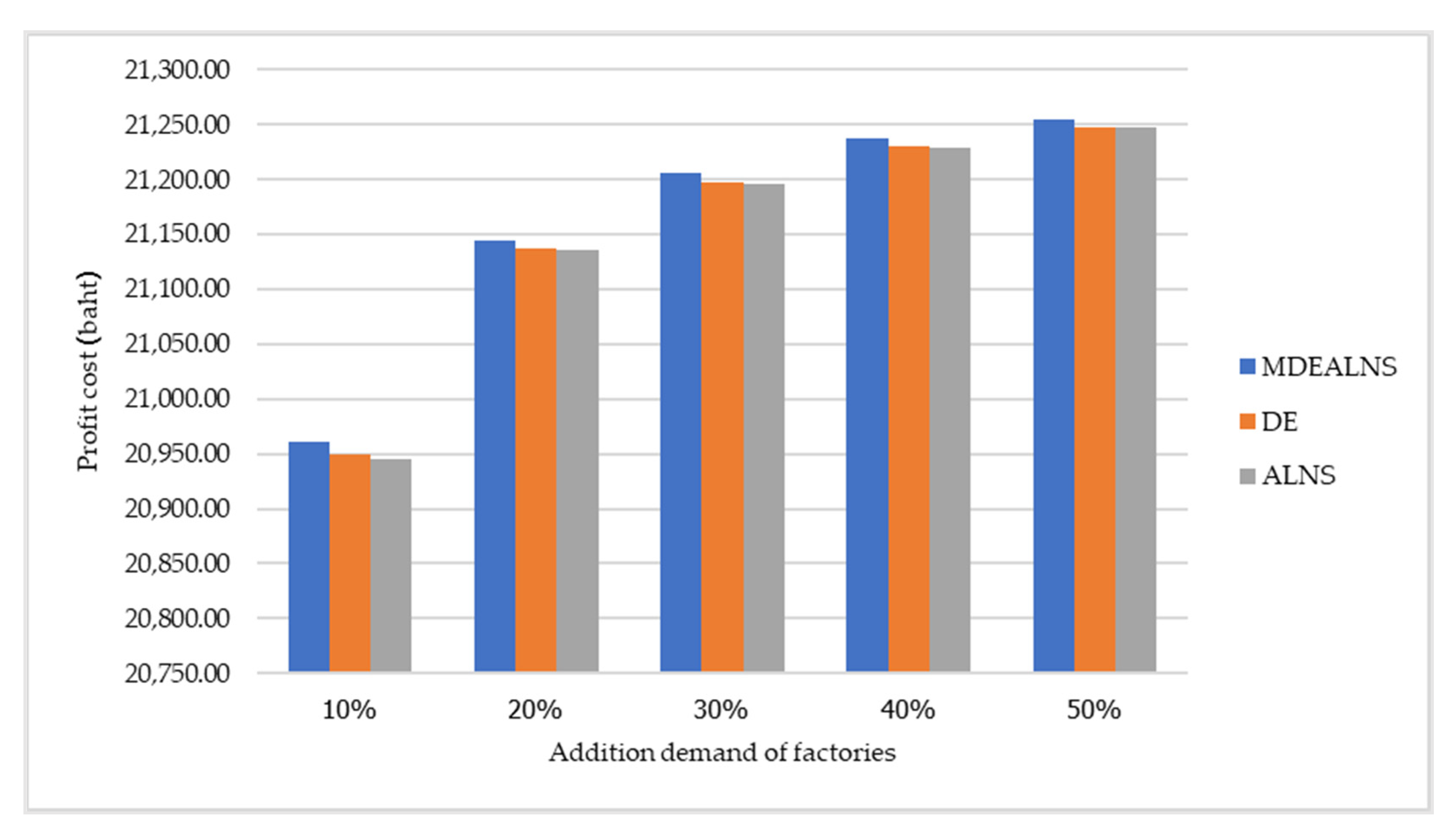
| Addition Demand of Factories (%) | Demand (tons) | Sell Cost (Bath) | MDEALNS | DE | ALNS | ||||||
|---|---|---|---|---|---|---|---|---|---|---|---|
| Shipping Cost (Bath) | Total Cost (Bath) | Profit (Bath) | Shipping Cost (Bath) | Total Cost (Bath) | Profit (Bath) | Shipping Cost (Bath) | Total Cost (Bath) | Profit (Bath) | |||
| 10% | 116.00 | 2,474,280.00 | 42,742 | 2,431,538.00 | 20,961.53 | 44,107 | 2,430,173.00 | 20,949.77 | 44,562 | 2,429,718.00 | 20,945.84 |
| 20% | 232.01 | 4,948,773.30 | 42,987 | 4,905,786.30 | 21,144.72 | 44,766 | 4,904,007.30 | 21,137.05 | 44,987 | 4,903,786.30 | 21,136.10 |
| 30% | 348.01 | 7,423,053.30 | 43,073 | 7,379,980.30 | 21,206.23 | 46,323 | 7,376,730.30 | 21,196.89 | 46,732 | 7,376,321.30 | 21,195.72 |
| 40% | 464.01 | 9,897,333.30 | 43,152 | 9,854,181.30 | 21,237.00 | 46,298 | 9,851,035.30 | 21,230.22 | 47,008 | 9,850,325.30 | 21,228.69 |
| 50% | 580.02 | 12,371,826.60 | 43,329 | 12,328,497.60 | 21,255.30 | 47,422 | 12,324,404.60 | 21,248.24 | 47,612 | 12,324,214.60 | 21,247.91 |
| Average | 348.01 | 7,423,053.30 | 43,057 | 7,379,996.70 | 21,160.96 | 45,783 | 7,377,270.10 | 21,152.43 | 46,180 | 7,376,873.10 | 21,150.85 |
Publisher’s Note: MDPI stays neutral with regard to jurisdictional claims in published maps and institutional affiliations. |
© 2022 by the authors. Licensee MDPI, Basel, Switzerland. This article is an open access article distributed under the terms and conditions of the Creative Commons Attribution (CC BY) license (https://creativecommons.org/licenses/by/4.0/).
Share and Cite
Chueadee, C.; Kriengkorakot, P.; Kriengkorakot, N. MDEALNS for Solving the Tapioca Starch Logistics Network Problem for the Land Port of Nakhon Ratchasima Province, Thailand. Logistics 2022, 6, 72. https://doi.org/10.3390/logistics6040072
Chueadee C, Kriengkorakot P, Kriengkorakot N. MDEALNS for Solving the Tapioca Starch Logistics Network Problem for the Land Port of Nakhon Ratchasima Province, Thailand. Logistics. 2022; 6(4):72. https://doi.org/10.3390/logistics6040072
Chicago/Turabian StyleChueadee, Chakat, Preecha Kriengkorakot, and Nuchsara Kriengkorakot. 2022. "MDEALNS for Solving the Tapioca Starch Logistics Network Problem for the Land Port of Nakhon Ratchasima Province, Thailand" Logistics 6, no. 4: 72. https://doi.org/10.3390/logistics6040072
APA StyleChueadee, C., Kriengkorakot, P., & Kriengkorakot, N. (2022). MDEALNS for Solving the Tapioca Starch Logistics Network Problem for the Land Port of Nakhon Ratchasima Province, Thailand. Logistics, 6(4), 72. https://doi.org/10.3390/logistics6040072