
The Development of a Digital Twin to Improve the Quality and Safety Issues of Cambodian Pâté: The Application of 915 MHz Microwave Cooking

 , , and
Abstract
1. Introduction
2. Materials and Methods
2.1. Tylose Preparation
2.2. Cambodian Pâté Preparation
2.3. Dielectric Properties’ Measurements
2.4. Thermal Conductivity Measurements
2.5. Heat Capacity Measurements
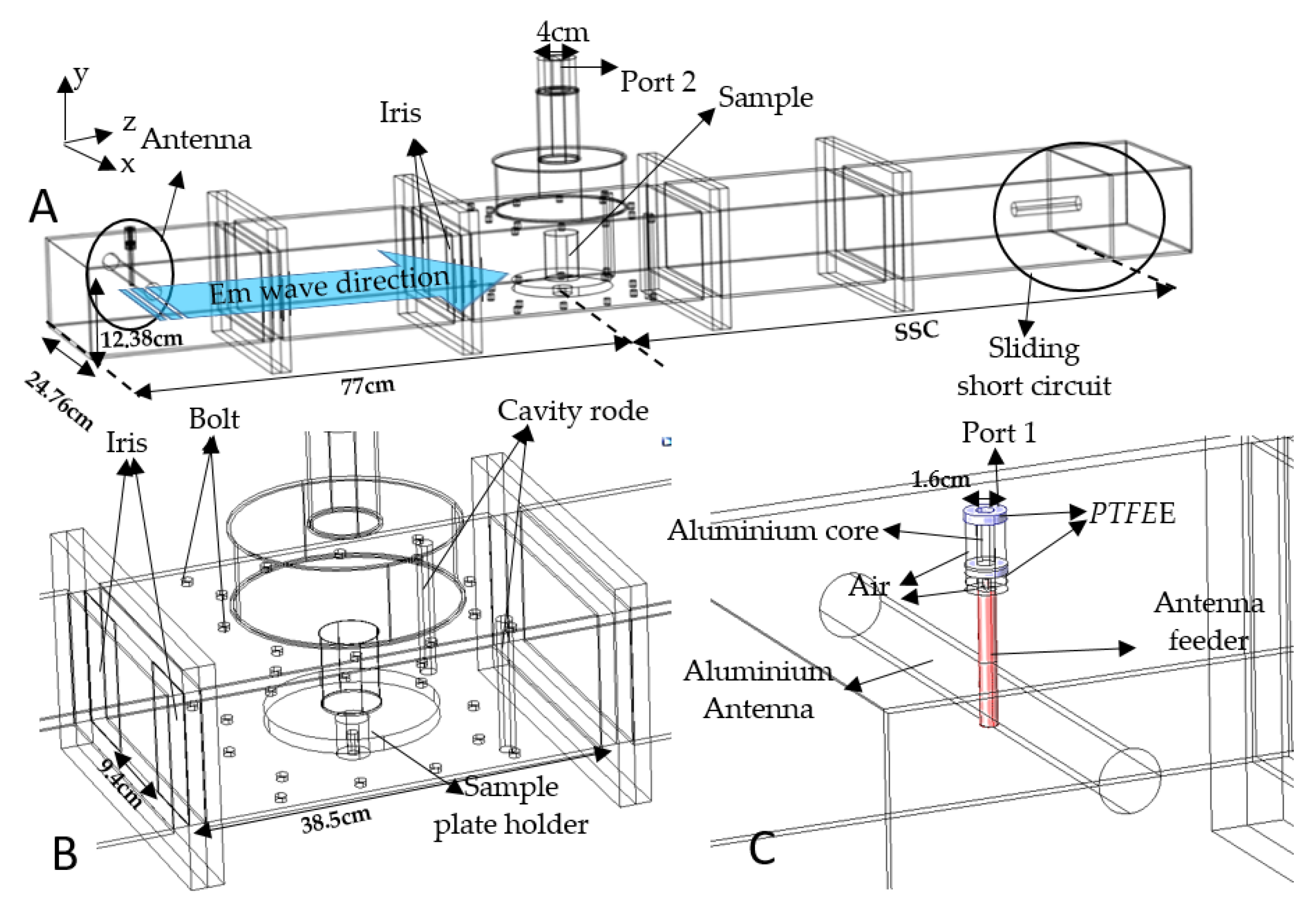
2.6. Microwave Device Configuration
2.7. Impedance-Matching Characterization
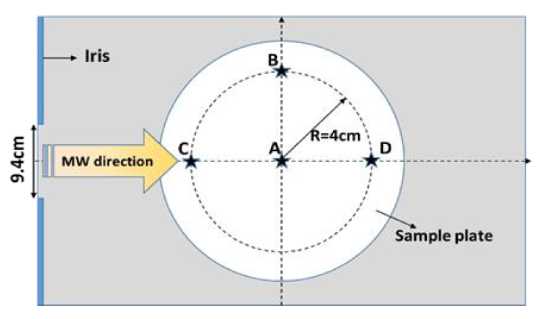
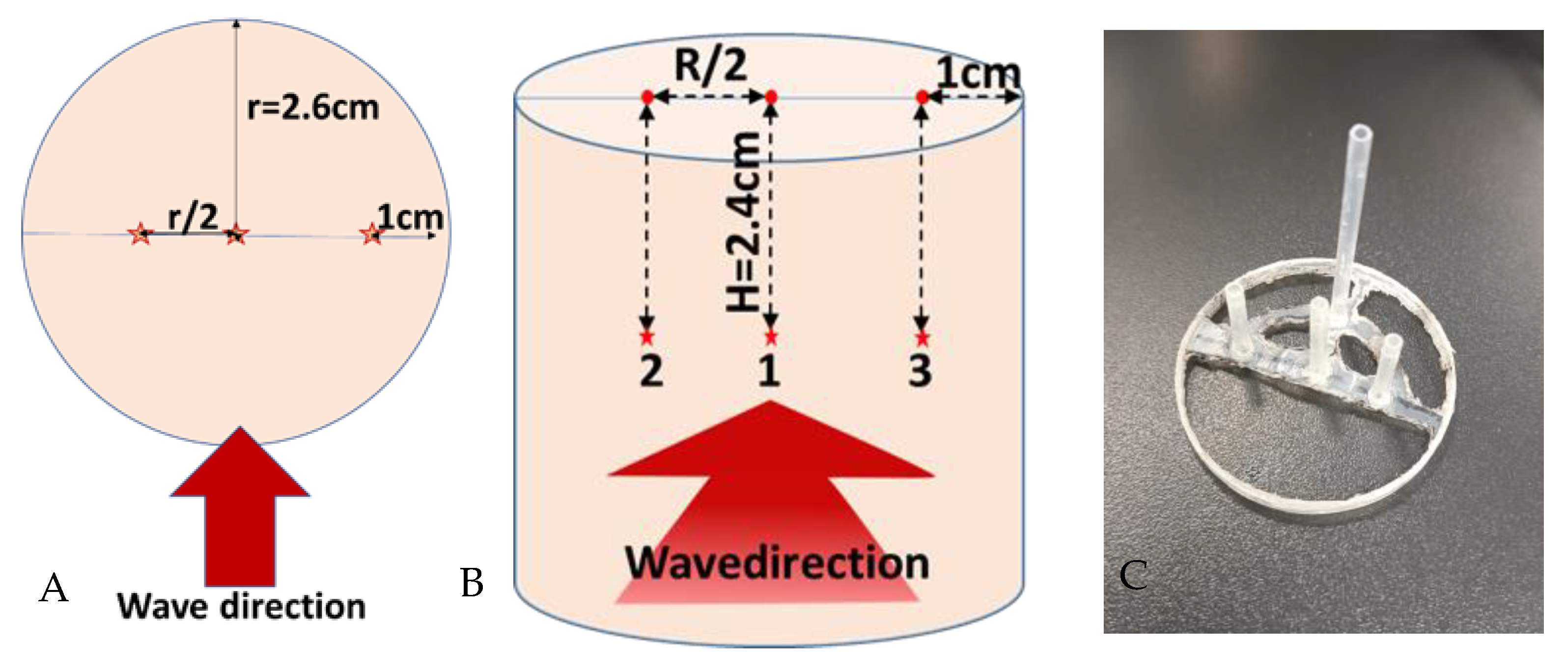
2.8. Microwave-Heating Experiments
2.9. Moisture Loss Characterization
2.10. Infrared Image
3. Modeling
3.1. Assumptions
- Tylose and raw pâté were considered homogenous and isotropic [10].
- The samples had homogenous initial temperatures [10].
- The thermophysical and dielectric properties of Tylose® were constant within the temperature range of the experiment [15].
- The thermal conductivity and dielectric properties of the pâté were a function of temperature, while the specific heat capacity of the pâté was assumed to be constant within the range of temperatures assessed.
- Thermal conductivity was constant within the variation range of moisture.
- Density was considered constant throughout the process [15].
- The shrinkage of the samples was considered negligible throughout the process [10].
- The bottom of the sample in contact with the PTFE support was considered thermally insulated.
- The sample was in perfect contact with the PET container.
- The ambient air was at a constant temperature (Tair = 293.15 K).
- The absolute humidity of the air surrounding the sample was constant throughout the experiment due to a small amount of evaporation from the sample into the air inside the microwave cavity.
3.2. Modeling of Microwave Propagation
- -
- Initial condition E = 0, t = 0.
- -
- The boundary condition for the TE10 mode:
- Ex = 0 at y = 0;
- Ex = 0 at y = 12.38 cm (width of the waveguide);
- Ey = 0 at x = 0;
- Ey = 0 at x = 24.76 cm (height of the waveguide);
- Ez = 0.
- -
- The impedance boundary condition is used at the walls of the waveguides for brass, copper, and aluminum metallic surfaces [17]
- -
- Perfect electrical conductor: apply to the surface of the metallic core inside the PTFE ring of the antenna (n × E = 0).
- -
- Port boundary condition: the percentage values of microwave reflected power (RF) at the input port (coaxial port for antenna) and port 2 were calculated from the squared magnitude values of S11 and S21 [16]. The S-parameter values at both ports are:
3.3. Heat Transfer
- -
- Initial condition: T0 = 4 °C, t = 0.
- -
- The boundary condition for the top surface of the sample involves both evaporation and natural convection phenomena [22]:
- -
- The boundary values for the side surface of PET sample cells are:
3.4. Mass Transfer
- -
- Initial condition:
- -
- At the top surface of the sample, the boundary equation is expressed as:
- -
- At the bottom and the lateral surfaces, no evaporation occurred. The equation for this boundary is:
- -
- The moisture loss is calculated from the following expression:
3.5. Thermophysical and Dielectric Properties

| Surface Boundary | Electrical Conductivity | Reference |
|---|---|---|
| Aluminum | 3.774·107 S/m | COMSOL® database |
| Brass | 1.59·107 S/m | [38] |
| Copper | 5.99·107 S/m | COMSOL® database |
| Parameters | Value/Units | References |
|---|---|---|
| RH | 0.3 | [47] |
| % dry matter | 23.52% | Measure |
| me | 0.02 | [22] |
| h0 | 2501·103 J/kg | [29] |
| Da | 2.5·10−8 (m2·s−1) | [48] |
| Km | 1.29·10−9 (kg·m−1·s−1) | [22] |
| Cpd.a | 1005 J/(kg·K) | [29] |
| Cpm | 1870 J/(kg·K) | [29] |
| Cm | 0.003 kg/kg | [22,49] |
| Z | 0.999 | [30] |
| α | 1.0062 | [30] |
| β | [30] | |
| γ | [30] | |
| A | 1.2811805 | [30] |
| B | −1.9509874 | [30] |
| C | 34.04926034 | [30] |
| D | −6.3536311 | [30] |
4. Model Design
4.1. Computational Details
4.2. Mesh Configuration
4.3. Validation Method
5. Results and Discussion
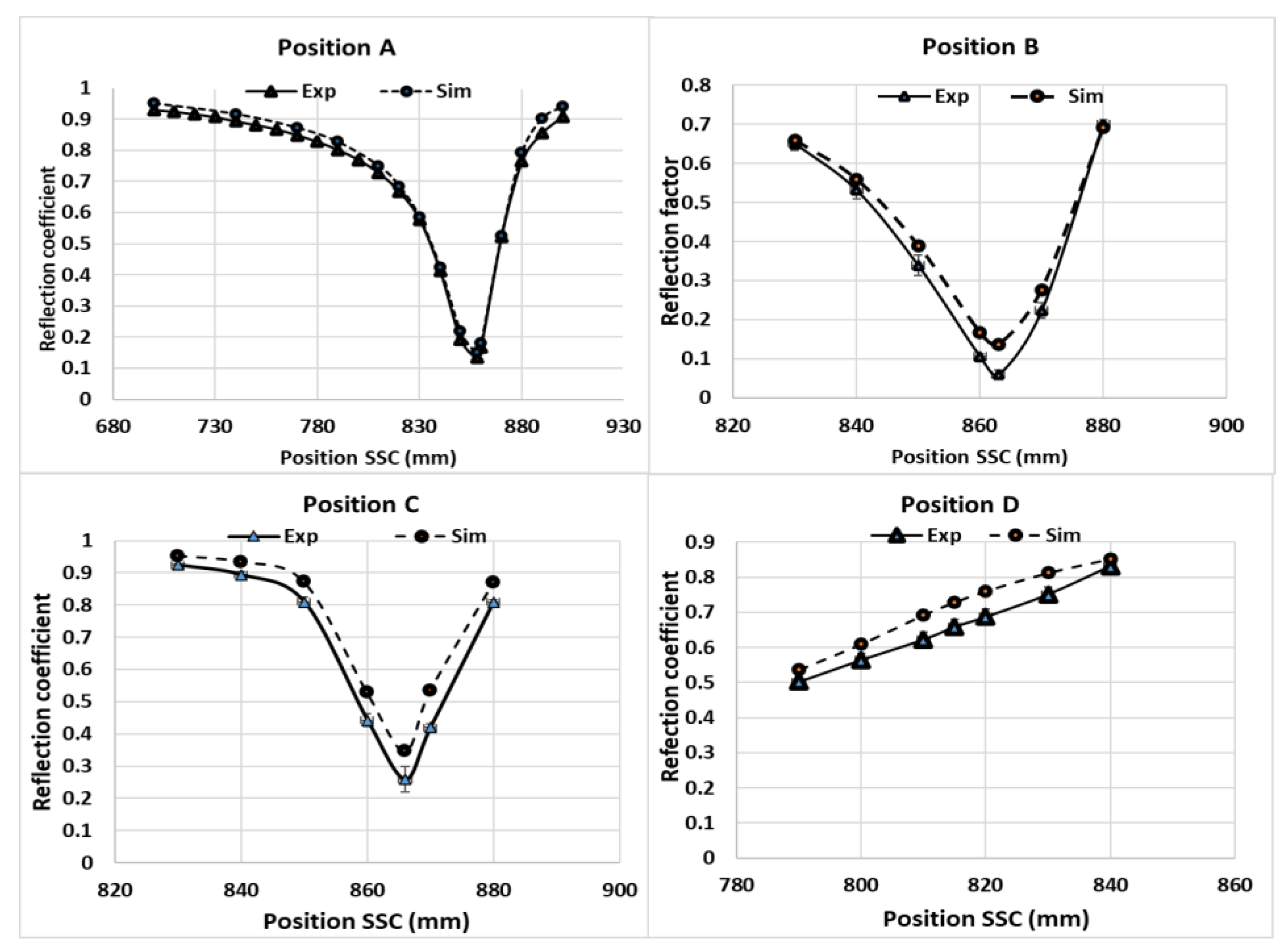
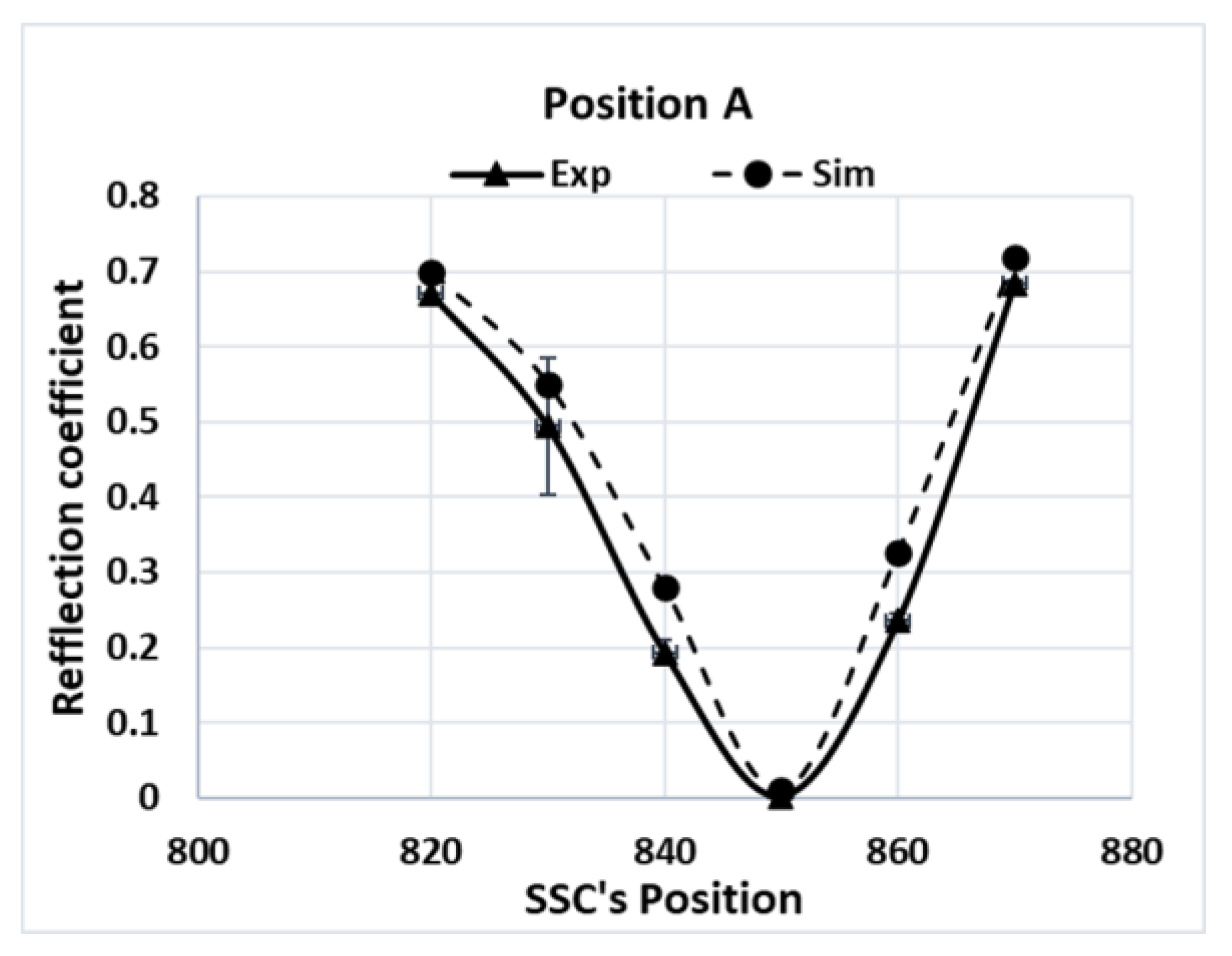
5.1. Electromagnetic Validation
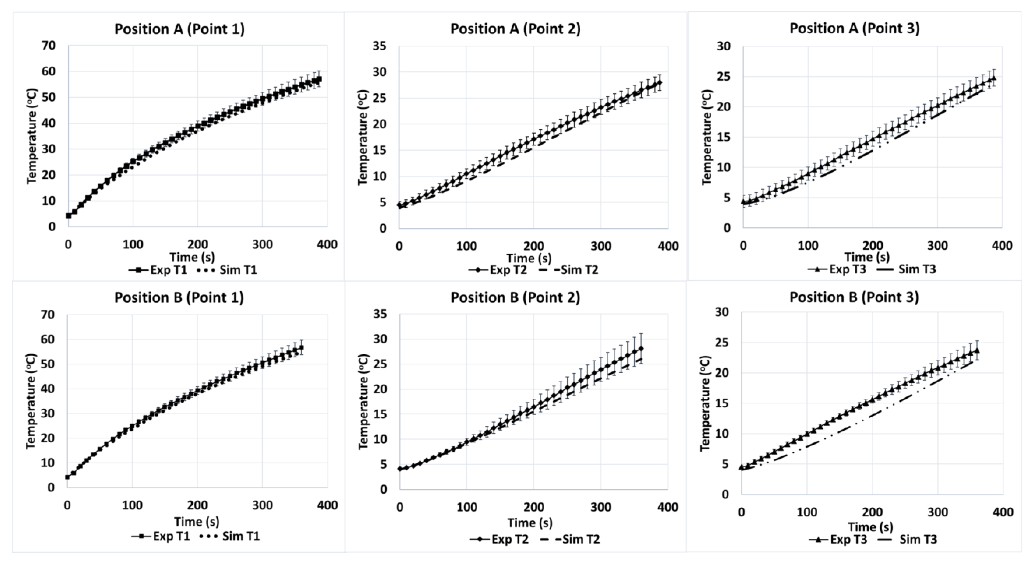
5.2. Temperature Validation
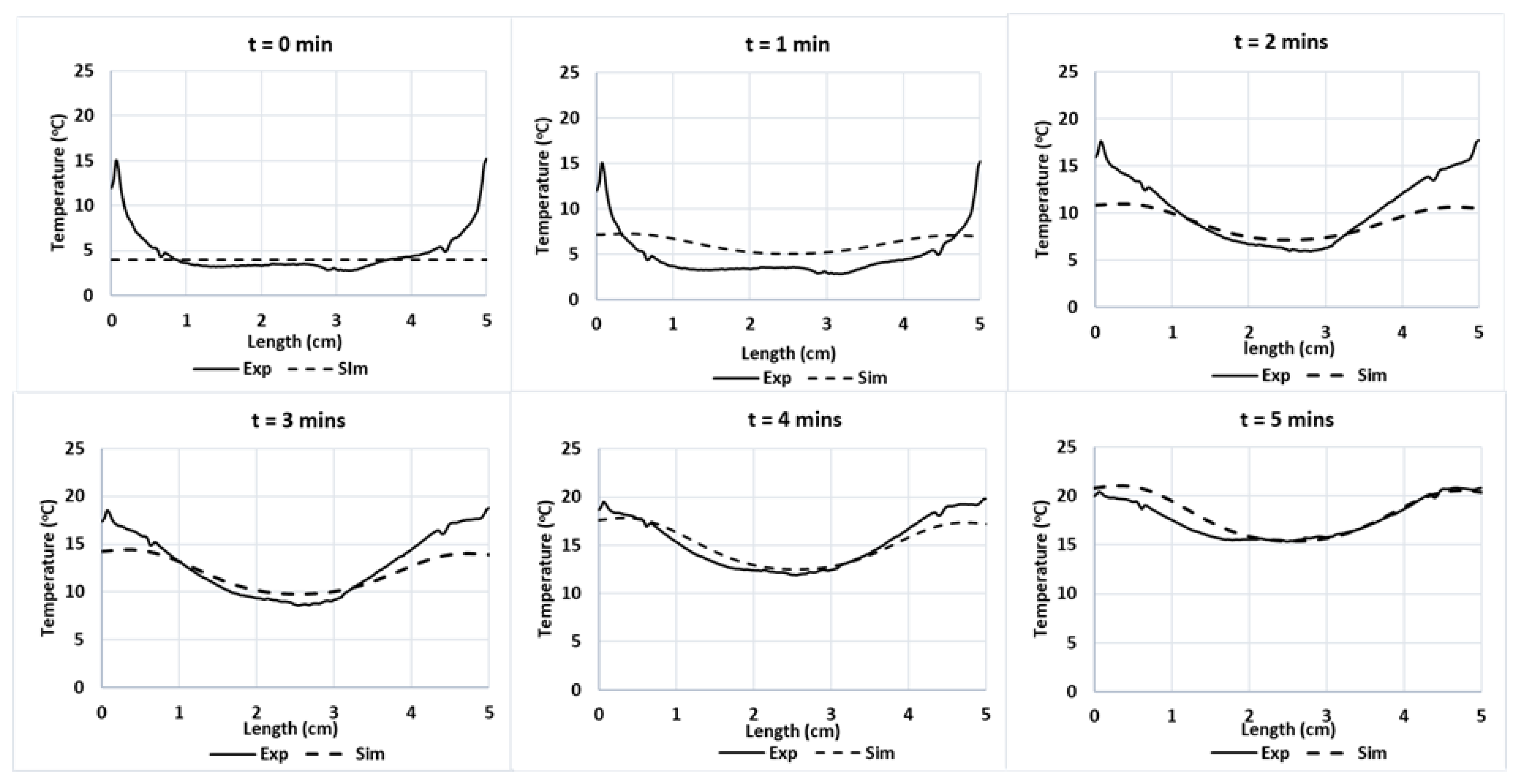
5.2.1. Tylose
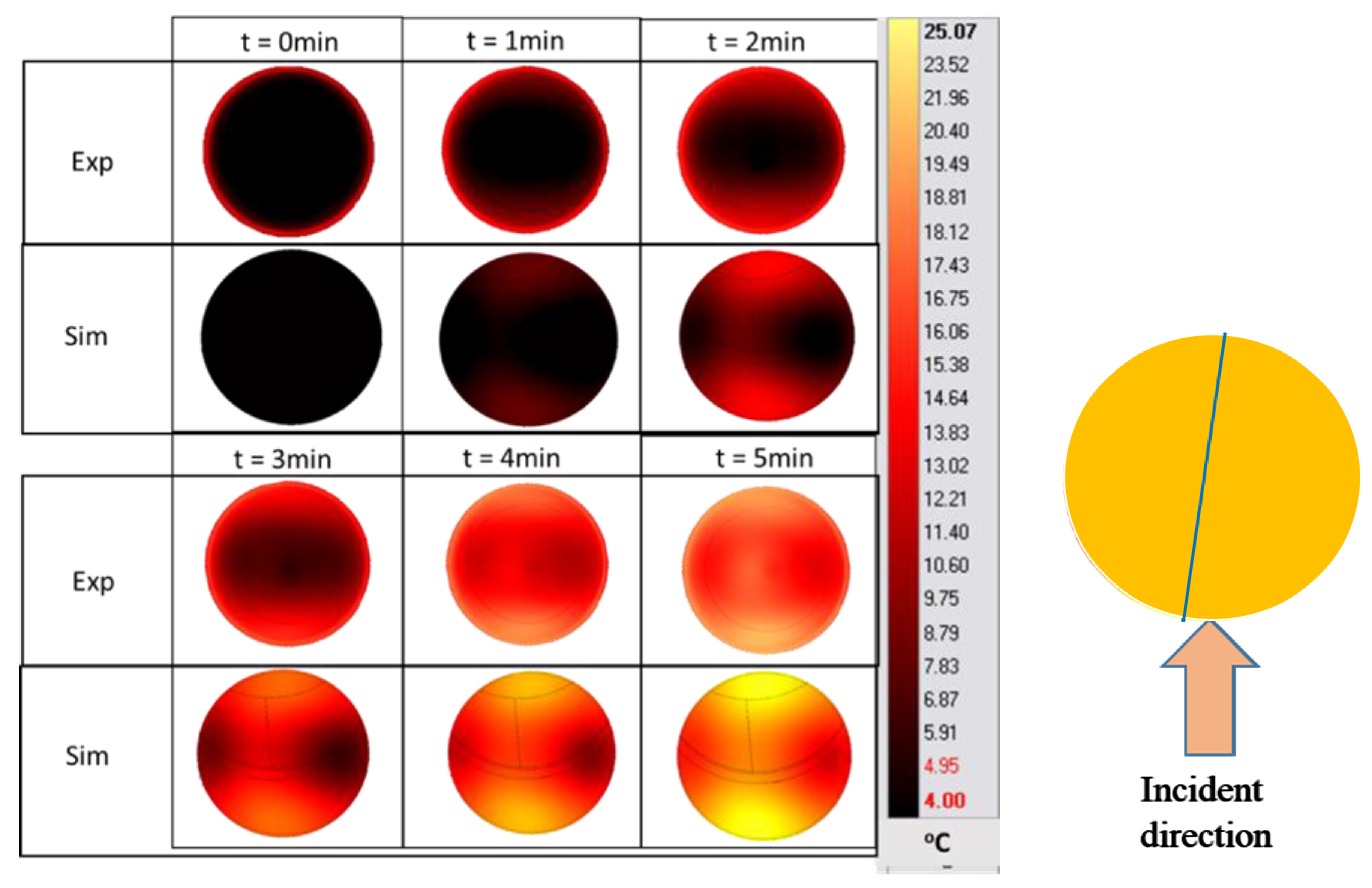
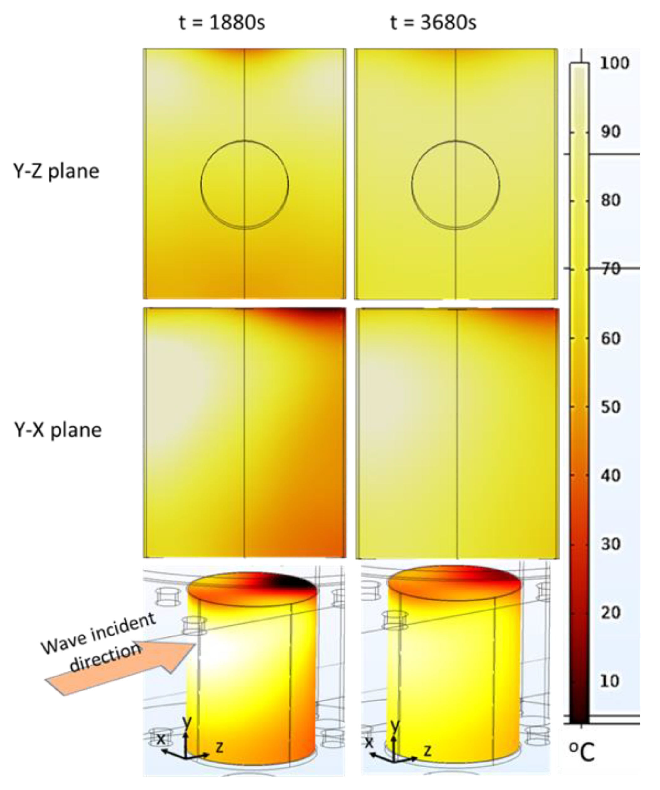
5.2.2. Cambodian Pâté
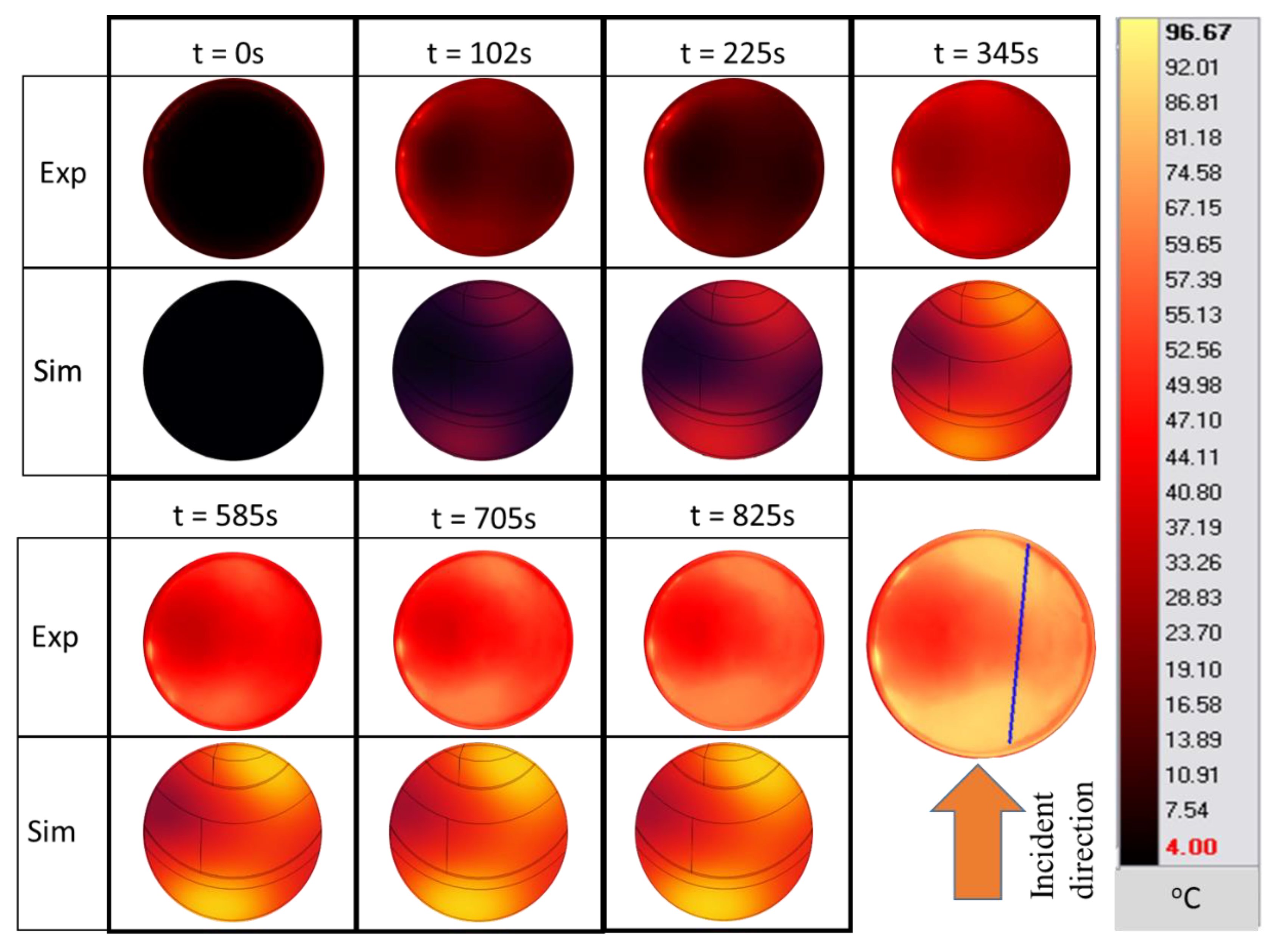
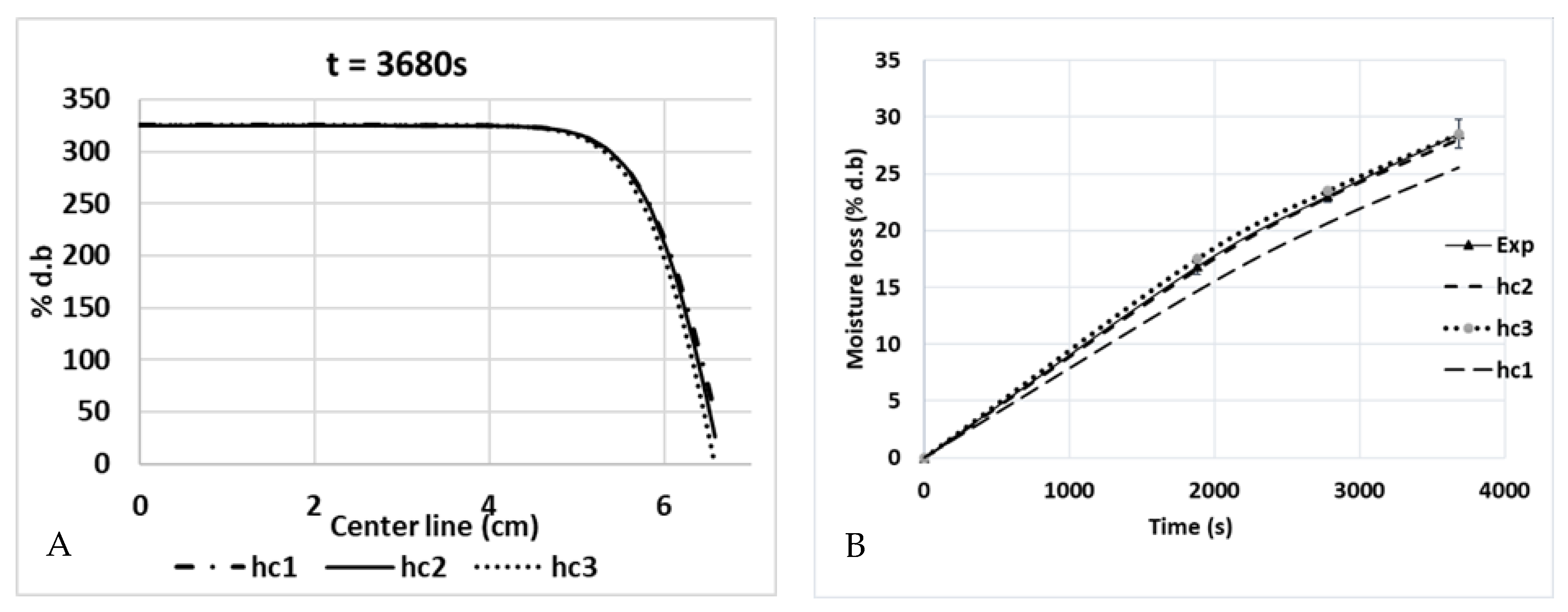
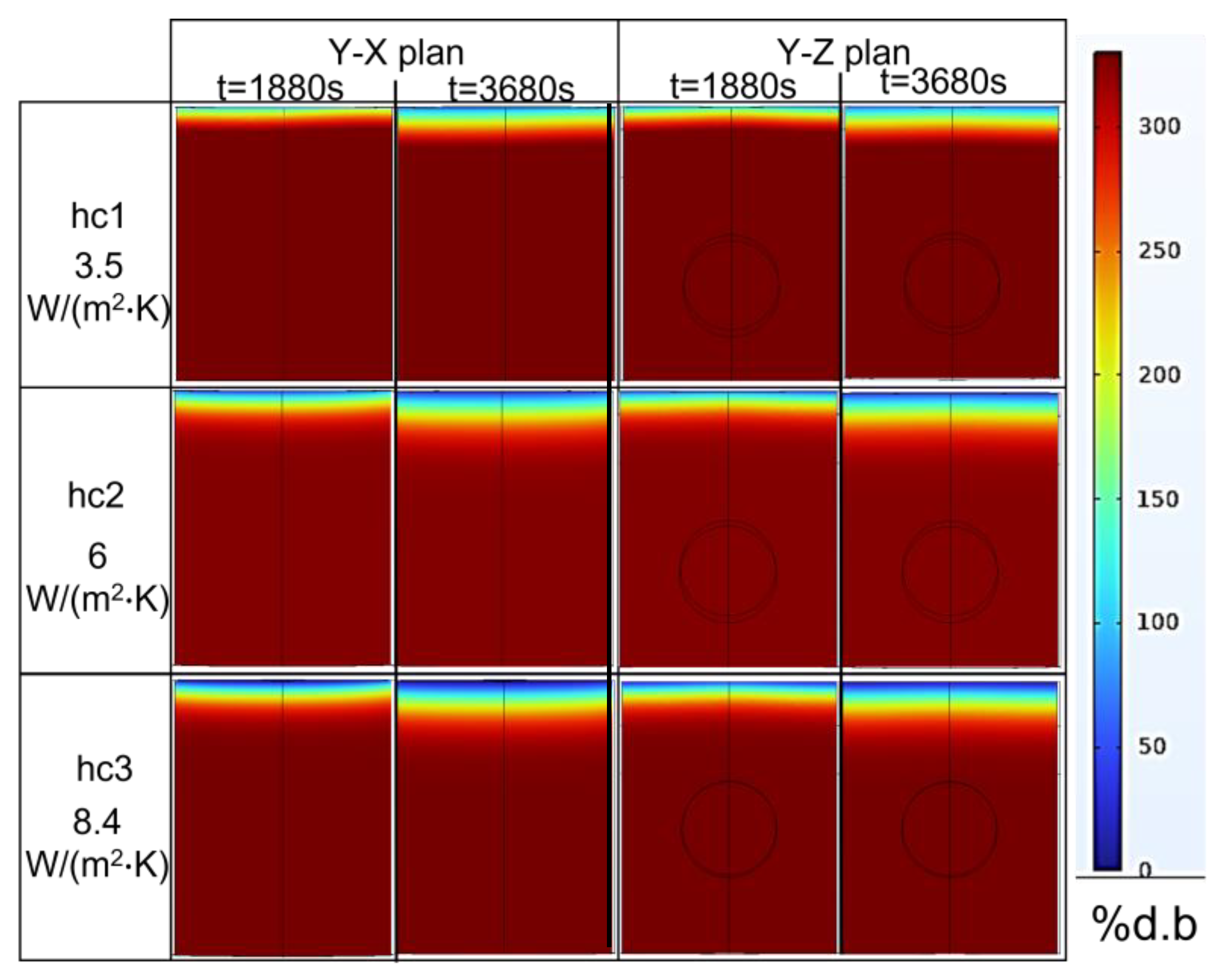
5.3. Mass Transfer Validation
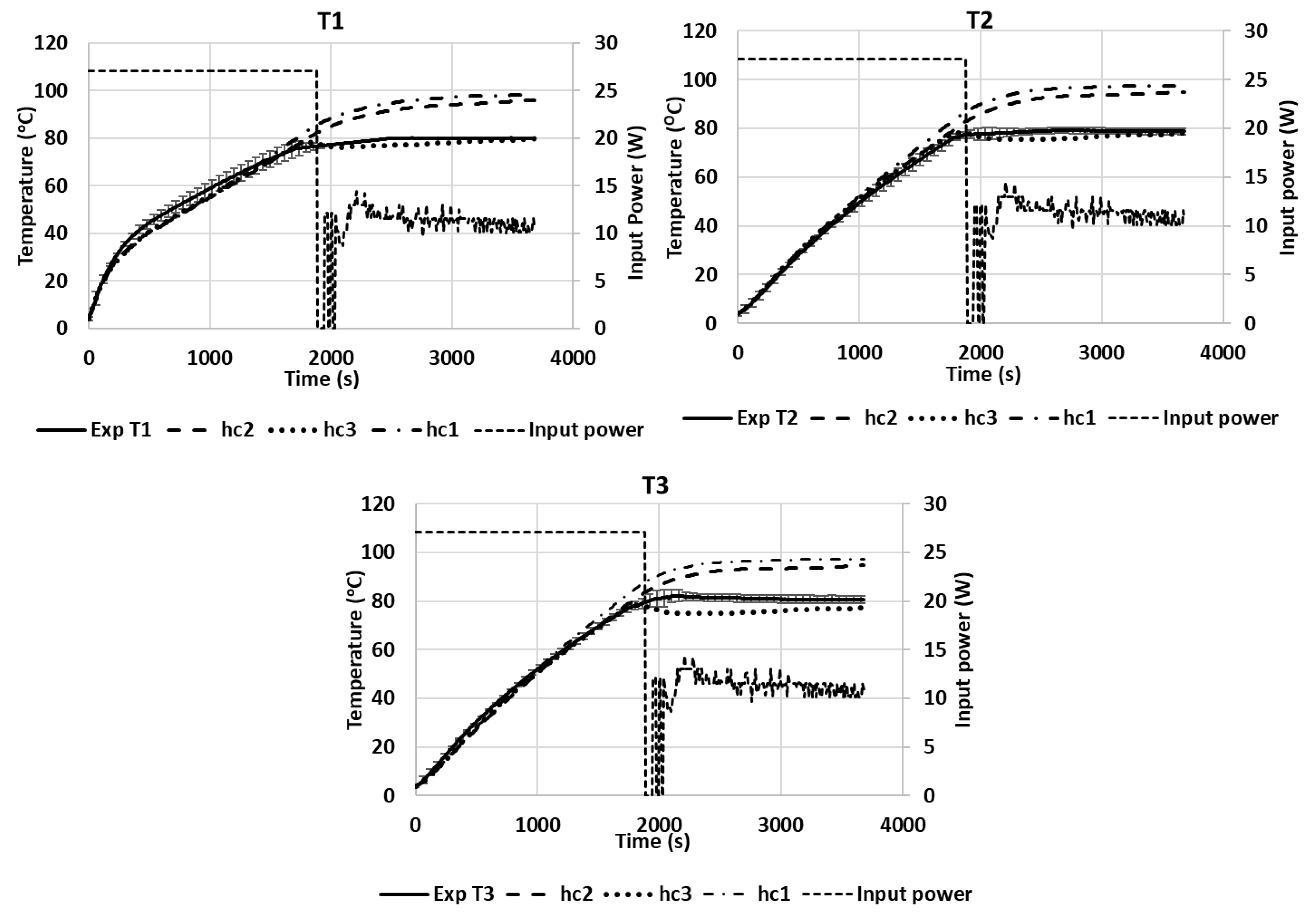
5.4. Sensitivity Analysis
6. Conclusions
Author Contributions
Funding
Data Availability Statement
Acknowledgments
Conflicts of Interest
Abbreviations
| Dielectric loss factor | |
| Relative permittivity | |
| Air density (kg/m3), | |
| ρs | Density of the food product (kg/m3) |
| µ | Magnetic permeability (H/m) |
| µo | Magnetic permeability of vacuum 4π × 10−7 H/m |
| Cb | Equilibrium moisture concentration (mol/m3) |
| Cm | Specific moisture capacity (kgmoisture/kgfood) |
| Cp | Specific heat capacity of the sample (J · kg−1·K−1) |
| Cpa | Heat capacity of the air (J·kg−1·K−1) |
| Cpd.a | Heat capacity of dried air 1005 J/(kg·K), |
| Cpm | Heat capacity of water vapor 1870 J/(kg·K) |
| Cw | Moisture concentration at the surface of food material (mol/m3) |
| d | Humidity ratio in mass (kg moisture/kg dry air) |
| Da | Air-diffusion coefficient of water vapor in the air (10−11 m2/s) |
| d.b | Dry base matter |
| Dm | Moisture diffusivity (m2/s) |
| E | Electric field (V/m) |
| Ec | Calculated electric field |
| E1 | Analytic field of excitation port |
| E2 | Eigenmode calculated from the boundary mode analysis and normalized concerning the outgoing power flow |
| E* | Complex conjugate electric field |
| ε | Complex permittivity of the material |
| εo | |
| f | Microwave frequency (Hz) |
| f’ | Correction function |
| hc | Convective heat-transfer coefficient (W·m−2·K−1) |
| ha | Enthalpy of dry air (J·kg−1) |
| h0 | Enthalpy of vaporization at 0 °C (J·kg−1) |
| hm | Convective mass-transfer coefficient (kg/(m2·s)) |
| hf | Enthalpy of hot-air film (J·kg−1) |
| hv | Enthalpy of water vapor (J·kg−1) |
| Latent heat of vaporization of liquid water (J·kg−1) | |
| i | Complex number |
| ka | Thermal conductivity of air (W ·m−1·K−1) |
| kc | Mass-transfer coefficient (m/s) |
| le | Lewis number |
| me | Equilibrium moisture content of air, decimal wet basis |
| mf | Mass of sample after heating process (kg) |
| mml | Amount of moisture loss (% d.b) |
| m0 | Mass of sample before heating process (kg) |
| Mw | Molar mass of water (kg/mol) |
| psv | Saturation pressure of vapor (Pa) |
| Qev | Heat loss due to evaporation (W·m−2) |
| RH | Relative humidity of surrounding air |
| rd | Ratio of dry matter in wet sample (kg dry matter/kg wet product) |
| Ta | Temperature of the hot-air film (K) |
| Tair | Ambient air temperature (293.15 K) |
| Text | External temperature (K) |
| Ts | Temperature at the surface of food material (K) |
| X1 | Value of analyzing parameter received from first data comparison |
| X2 | Value of analyzing parameter received from second data comparison |
| xsv | Mole fraction of saturated water vapor |
| Xv | Mole fraction of moisture inside the air (molwater/moldry air) |
| Latent heat of vaporization of water (J/mol) |
References
- De Albuquerque, C.D.; Curet, S.; Boillereaux, L. Influence of heating rate during microwave pasteurization of ground beef products: Experimental and numerical study. J. Food Process Eng. 2021, 44, e13722. [Google Scholar] [CrossRef]
- Cheng, T.; Tang, J.; Yang, R.; Xie, Y.; Chen, L.; Wang, S. Methods to obtain thermal inactivation data for pathogen control in low-moisture foods. Trends Food Sci. Technol. 2021, 112, 174–187. [Google Scholar] [CrossRef]
- Klinbun, W.; Rattanadecho, P. Numerical study of initially frozen rice congee with thin film resonators package in microwave domestic oven. J. Food Process Eng. 2022, 45, e13924. [Google Scholar] [CrossRef]
- Pitchai, K.; Chen, J.; Birla, S.; Jones, D.; Gonzalez, R.; Subbiah, J. Multiphysics modeling of microwave heating of a frozen heterogeneous meal rotating on a turntable. J. Food Sci. 2015, 80, E2803–E2814. [Google Scholar] [CrossRef] [PubMed]
- Zhu, H.; Gulati, T.; Datta, A.K.; Huang, K. Microwave drying of spheres: Coupled electromagnetics-multiphase transport modeling with experimentation. Part I: Model development and experimental methodology. Food Bioprod. Process. 2015, 96, 314–325. [Google Scholar] [CrossRef]
- Shen, L.; Gao, M.; Feng, S.; Ma, W.; Zhang, Y.; Liu, C.; Liu, C.; Zheng, X. Analysis of heating uniformity considering microwave transmission in stacked bulk of granular materials on a turntable in microwave ovens. J. Food Eng. 2022, 319, 110903. [Google Scholar] [CrossRef]
- Chen, J.; Pitchai, K.; Birla, S.; Jones, D.; Negahban, M.; Subbiah, J. Modeling heat and mass transport during microwave heating of frozen food rotating on a turntable. Food Bioprod. Process. 2016, 99, 116–127. [Google Scholar] [CrossRef]
- Gulati, T.; Zhu, H.; Datta, A.K. Coupled electromagnetics, multiphase transport and large deformation model for microwave drying. Chem. Eng. Sci. 2016, 156, 206–228. [Google Scholar] [CrossRef]
- Ye, J.; Lan, J.; Xia, Y.; Yang, Y.; Zhu, H.; Huang, K. An approach for simulating the microwave heating process with a slow- rotating sample and a fast-rotating mode stirrer. Int. J. Heat Mass Transf. 2019, 140, 440–452. [Google Scholar] [CrossRef]
- Siguemoto, É.S.; Gut, J.A.W.; Dimitrakis, G.; Curet, S.; Boillereaux, L. Evaluation of microwave applicator design on electromagnetic field distribution and heating pattern of cooked peeled shrimp. Foods 2021, 10, 1903. [Google Scholar] [CrossRef]
- Zhou, X.; Pedrow, P.D.; Tang, Z.; Bohnet, S.; Sablani, S.S.; Tang, J. Heating performance of microwave ovens powered by magnetron and solid-state generators. Innov. Food Sci. Emerg. Technol. 2023, 83, 103240. [Google Scholar] [CrossRef]
- Llave, Y.; Mori, K.; Kambayashi, D.; Fukuoka, M.; Sakai, N. Dielectric properties and model food application of tylose water pastes during microwave thawing and heating. J. Food Eng. 2016, 178, 20–30. [Google Scholar] [CrossRef]
- Zhang, Z.; Su, T.; Zhang, S. Shape Effect on the Temperature Field during Microwave Heating Process. J. Food Qual. 2018, 2018, 9169875. [Google Scholar] [CrossRef]
- Nget, S.; Mith, H.; Curet, S.; Boillereaux, L. Reflection Coefficient-Based Validation of Electromagnetic Model: Application to Model Food at 915 MHz. In Proceedings of the 36th Annual European Simulation and Modelling Conference (ESM® 2022), Porto, Portugal, 26–28 October 2022; pp. 165–169. [Google Scholar]
- de Albuquerque, C.D.; Curet, S.; Boillereaux, L. A 3D-CFD-heat-transfer-based model for the microbial inactivation of pasteurized food products. Innov. Food Sci. Emerg. Technol. 2019, 54, 172–181. [Google Scholar] [CrossRef]
- Curet, S.; Rouaud, O.; Boillereaux, L. Effect of Sample Size on Microwave Power Absorption within Dielectric Materials: 2D Numerical Results vs. Closed-Form Expressions. AIChE J. 2009, 55, 1569–1583. [Google Scholar] [CrossRef]
- Tauhiduzzaman, M.; Hafez, I.; Bousfield, D.; Tajvidi, M. Modeling microwave heating and drying of lignocellulosic foams through coupled electromagnetic and heat transfer analysis. Processes 2021, 9, 2001. [Google Scholar] [CrossRef]
- Chen, J.; Lau, S.K.; Chen, L.; Wang, S.; Subbiah, J. Modeling radio frequency heating of food moving on a conveyor belt. Food Bioprod. Process. 2017, 102, 307–319. [Google Scholar] [CrossRef]
- Thuto, W.; Banjong, K. Investigation of heat and moisture transport in bananas during microwave heating process. Processes 2019, 7, 545. [Google Scholar] [CrossRef]
- Datta, A.K.; Anantheswaran, R. The Handbook of Microwave Technology for Food Applications; CRC Press: Boca Raton, FL, USA, 2001; Volume 1. [Google Scholar]
- Bennamoun, L.; Li, J. Drying Process of Food: Fundamental Aspects and Mathematical Modeling; Elsevier Inc.: Amsterdam, The Netherlands, 2018; Volume 2. [Google Scholar]
- Chen, H.; Marks, B.P.; Murphy, R.Y. Modeling coupled heat and mass transfer for convection cooking of chicken patties. J. Food Eng. 1999, 42, 139–146. [Google Scholar] [CrossRef]
- Luikov, A.V. Heat and Mass Transfer in Capillary-Porous Bodies, 1st ed.; The Academy of Science, BSSR, Mink: Oxford, UK; London, UK; Edinburgh, UK; New York, NY, USA; Paris, France; Frankfurt, Germany, 1966. [Google Scholar]
- Blikra, M.J.; Skipnes, D.; Feyissa, A.H. Model for heat and mass transport during cooking of cod loin in a convection oven. Food Control 2019, 102, 29–37. [Google Scholar] [CrossRef]
- Pham, Q.T.; Willix, J. A Model for Food Desiccation in Frozen Storage. J. Food Sci. 1984, 49, 1275–1281. [Google Scholar] [CrossRef]
- Enayatollahi, R.; Nates, R.J.; Anderson, T. The analogy between heat and mass transfer in low temperature crossflow evaporation. Int. Commun. Heat Mass Transf. 2017, 86, 126–130. [Google Scholar] [CrossRef]
- Henderson-Sellers, B. A new formula for latent heat of vaporization of water as a function of temperature. Q. J. R. Meteorol. Soc. 1984, 110, 1186–1190. [Google Scholar] [CrossRef]
- Tsilingiris, P.T. Review and critical comparative evaluation of moist air thermophysical properties at the temperature range between 0 and 100 °C for Engineering Calculations. Renew. Sustain. Energy Rev. 2018, 83, 50–63. [Google Scholar] [CrossRef]
- Zheng, H. Fundamental Relationships of Heat and Mass Transfer in Solar Seawater Desalination Systems. In Solar Energy Desalination Technology; Elsevier: Amsterdam, The Netherlands, 2017; pp. 173–258. [Google Scholar]
- Davis, R.S. Equation for the determination of the density of moist air (1981/91). Metrologia 1992, 29, 67–70. [Google Scholar] [CrossRef]
- Konieczna, M.; Markiewicz, E.; Jurga, J. Dielectric Properties of Polyethylene Terephthalate/Polyphenylene Sulfide/Barium Titanate Nanocomposite for Application in Electronic Industry. Polym. Eng. Sci. 2010, 52, 1613–1619. [Google Scholar] [CrossRef]
- Sandhu, M.Y.; Ali, A.; Hunter, I.C.; Roberts, N.S. A new method for the precise multiband microwave dielectric measurement using stepped impedance stub. Meas. Sci. Technol. 2016, 27, 117001. [Google Scholar] [CrossRef]
- Aleem, A.; Ghaffar, A.; Kiani, N.M.; Irshad, M.; Mehmood, I.; Shahzad, M.; Shahbaz, A. Broad-band dielectric properties of Teflon, Bakelite, air: Simulation and experimental study. Mater. Sci. Eng. B Solid-State Mater. Adv. Technol. 2021, 272, 115347. [Google Scholar] [CrossRef]
- Barringer, S.; Bircan, C. Dielectric properties and protien denaturation.pdf. In Advances in Microwave and Radio Frequency Processing, 1st ed.; Willert-Porada, M., Ed.; Springer: Berlin/Heidelberg, Germany; New York, NY, USA, 2006; pp. 107–118. [Google Scholar]
- Ngadi, M.; Dev, S.R.S.; Raghavan, V.G.S.; Kazemi, S. Dielectric Properties of Pork Muscle. Int. J. Food Prop. 2015, 18, 12–20. [Google Scholar] [CrossRef]
- Gezahegn, Y.A.; Tang, J.; Sablani, S.S.; Pedrow, P.D.; Hong, Y.-K.; Lin, H.; Tang, Z. Dielectric properties of water relevant to microwave assisted thermal pasteurization and sterilization of packaged foods. Innov. Food Sci. Emerg. Technol. 2021, 74, 102837. [Google Scholar] [CrossRef]
- Wipawee, T.; Witchuda, D.; Pitiya, K. Simulation of Thermal and Electric Field Distribution in. Food 2021, 10, 1622. [Google Scholar] [CrossRef]
- Muhammad, U.K.; Umar, S. Experimental Performance Investigations and Evaluation of Base Metals Thermocouples. Int. J. Mod. Appl. Phys. Int. J. Mod. App. Phys. 2013, 3, 26–37. Available online: https://www.researchgate.net/publication/325153687 (accessed on 15 May 2018).
- Nunes, L.C.S.; Dias, F.W.R.; Mattos, H.S.C. Mechanical behavior of polytetra fl uoroethylene in tensile loading under different strain rates. Polym. Test. 2011, 30, 791–796. [Google Scholar] [CrossRef]
- Furukawa, G.T.; Mccoskey, R.E.; King, G.J. Calorimetric properties of polytetrafluoroethylene (teflon) from 0-degrees to 365-degrees-K. J. Res. Natl. Bur. Stand. 1952, 49, 273. [Google Scholar] [CrossRef]
- Maddah, H.A. Polypropylene as a Promising Plastic: A Review. Am. J. Polym. Sci. 2016, 6, 1–11. [Google Scholar] [CrossRef]
- Weidenfeller, B.; Höfer, M.; Schilling, F.R. Thermal conductivity, thermal diffusivity, and specific heat capacity of particle filled polypropylene. Compos. Part A Appl. Sci. Manuf. 2004, 35, 423–429. [Google Scholar] [CrossRef]
- Weidenfeller, B.; Kirchberg, S. Thermal and mechanical properties of polypropylene-iron-diamond composites. Compos. Part B Eng. 2016, 92, 133–141. [Google Scholar] [CrossRef]
- Panowicz, R.; Konarzewski, M.; Durejko, T.; Szala, M.; Łazi, M. Properties of Polyethylene Terephthalate (PET) after Thermo-Oxidative Aging. Materials 2021, 14, 3833. [Google Scholar] [CrossRef]
- Lopes, C.M.A.; Felisberti, M.I. Thermal conductivity of PET/(LDPE/AI) composites determined by MDSC. Polym. Test. 2004, 23, 637–643. [Google Scholar] [CrossRef]
- Park, B.K.; Yi, N.; Park, J.; Kim, D. Monitoring protein denaturation using thermal conductivity probe. Int. J. Biol. Macromol. 2013, 52, 353–357. [Google Scholar] [CrossRef]
- Wypych, A.; Bochenek, B.; Rózycki, M. Atmospheric moisture content over Europe and the Northern Atlantic. Atmosphere 2018, 9, 18. [Google Scholar] [CrossRef]
- Huang, E.; Mittal, G.S. Meatball cooking—Modeling and simulation. J. Food Eng. 1995, 24, 87–100. [Google Scholar] [CrossRef]
- Scheerlinck, N.; Verboven, P.; Stigter, J.D.; Stigter, J.D.; Van Impe, J.F.; Nicolaï, B.M. Stochastic finite-element analysis of coupled heat and mass transfer problems with random field parameters. Numer. Heat Transf. Part B Fundam. 2000, 37, 309–330. [Google Scholar] [CrossRef]
- Zhang, Y.; Yang, H.; Yan, B.; Zhu, H.; Gao, W.; Zhao, J.; Chen, W.; Fan, D. Continuous flow microwave system with helical tubes for liquid food heating. J. Food Eng. 2021, 294, 110409. [Google Scholar] [CrossRef]
- Pitchai, K.; Chen, J.; Birla, S.; Gonzalez, R.; Jones, D.; Subbiah, J. A microwave heat transfer model for a rotating multi-component meal in a domestic oven: Development and validation. J. Food Eng. 2014, 128, 60–71. [Google Scholar] [CrossRef]
- Kosky, P.; Balmer, R.; Keat, W.; Wise, G. Chapter 14—Mechanical Engineering. In Exploring Engineering, 5th ed.; Academic Press: Cambridge, MA, USA, 2021; pp. 317–340. [Google Scholar] [CrossRef]


| Name | Equation | Reference |
|---|---|---|
| Latent heat of vaporization of liquid water | [27] | |
| Lewis number | [28] | |
| Heat capacity of the air around the sample | [28] | |
| Humidity ratio in mass | [29] | |
| Thermal conductivity of air around the sample | [29] | |
| The temperature of the hot-air film near the surface | [30] | |
| Mole fraction of moisture in the air | [30] | |
| Correction function | [30] | |
| Saturated pressure | [30] | |
| Air density | [30] | |
| Enthalpy of hot-air film | [29] | |
| Enthalpy of dry air | [29] | |
| Enthalpy of water vapor | [29] |
| Material | ε’r | ε″r | Reference |
|---|---|---|---|
| PET container | 3.5 | 0.0035 | [31] |
| PTFE | 2.1 | 0.002 | [32] |
| Air | 1 | 0 | [33] |
| Tylose | 69 | 8.9 | Measurement |
| Material | Density | Thermal Conductivity | Heat Capacity | References |
|---|---|---|---|---|
| Teflon | 2.2103 kg/m3 | 0.32 W/(m.K) | 1.02 J/(g.K) | [39,40] |
| Polypropylene | 930 kg/m3 | 0.3 W/(m.K) | 1.2 J/(g.K) | [41,42,43] |
| PET | 1380 kg/m3 | 0.2 W/(m.K) | 1.2 J/(g.K) | [44,45] |
| Tylose® | 965 kg/m3 | 0.5 W/(m.K) | 3859.9 J/(kg.K) | Measurement |
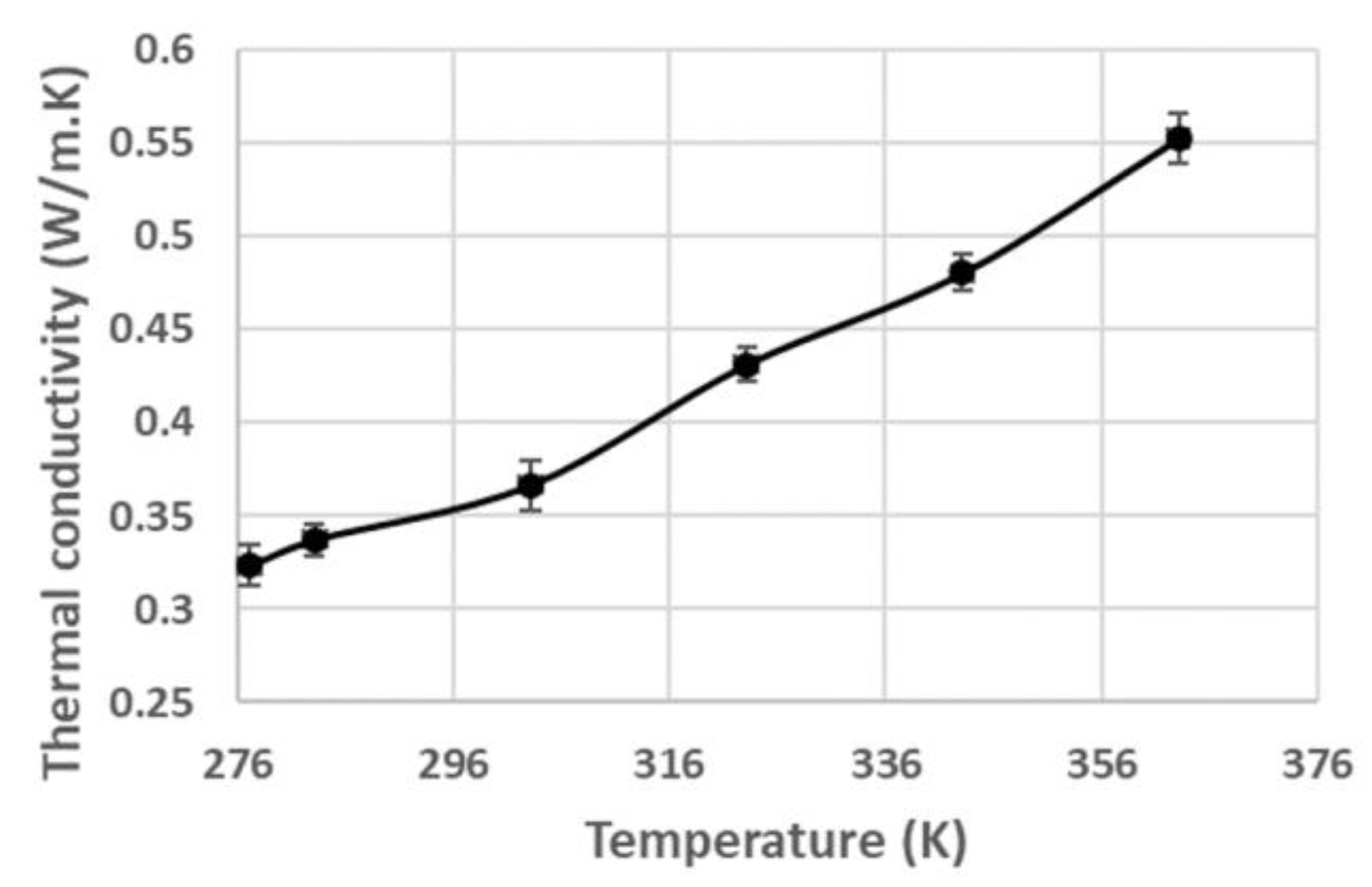
| Pâté | 903.6 kg/m3 | Figure 5 | 3511.3 J/(kg.K) | Measurement |
| Ramp-Up Heating RMSE/p-Value | Temperature-Holding Phase RMSE/p-Value | |
|---|---|---|
| Including mass transfer | ||
| hc1 and hc3 | 2.5603/p-value > 0.05 | 18.8437/p-value < 0.05 |
| hc2 and hc3 | 0.9630/p-value > 0.05 | 15.5992/p-value < 0.05 |
| hc1 and hc2 | 2.0257/p-value > 0.05 | 3.3303/p-value > 0.05 |
| Without mass transfer | ||
| hc1 and hc3 | 2.1473/p-value > 0.05 | |
| Comparing models with and without mass transfer | ||
| hc1 | 3.5680/p-value > 0.05 | 18.2840/p-value < 0.05 |
| hc3 | 8.2854/p-value < 0.05 | 31.0090/p-value < 0.05 |
| hc1 = 3.5 W/(m2·K), hc2 = 6 W/(m2·K), and hc3 = 8.4 W/(m2·K)). | ||
Disclaimer/Publisher’s Note: The statements, opinions and data contained in all publications are solely those of the individual author(s) and contributor(s) and not of MDPI and/or the editor(s). MDPI and/or the editor(s) disclaim responsibility for any injury to people or property resulting from any ideas, methods, instructions or products referred to in the content. |
© 2023 by the authors. Licensee MDPI, Basel, Switzerland. This article is an open access article distributed under the terms and conditions of the Creative Commons Attribution (CC BY) license (https://creativecommons.org/licenses/by/4.0/).
Share and Cite
Nget, S.; Mith, H.; Boué, G.; Curet, S.; Boillereaux, L. The Development of a Digital Twin to Improve the Quality and Safety Issues of Cambodian Pâté: The Application of 915 MHz Microwave Cooking. Foods 2023, 12, 1187. https://doi.org/10.3390/foods12061187
Nget S, Mith H, Boué G, Curet S, Boillereaux L. The Development of a Digital Twin to Improve the Quality and Safety Issues of Cambodian Pâté: The Application of 915 MHz Microwave Cooking. Foods. 2023; 12(6):1187. https://doi.org/10.3390/foods12061187
Chicago/Turabian StyleNget, Sovannmony, Hasika Mith, Géraldine Boué, Sébastien Curet, and Lionel Boillereaux. 2023. "The Development of a Digital Twin to Improve the Quality and Safety Issues of Cambodian Pâté: The Application of 915 MHz Microwave Cooking" Foods 12, no. 6: 1187. https://doi.org/10.3390/foods12061187
APA StyleNget, S., Mith, H., Boué, G., Curet, S., & Boillereaux, L. (2023). The Development of a Digital Twin to Improve the Quality and Safety Issues of Cambodian Pâté: The Application of 915 MHz Microwave Cooking. Foods, 12(6), 1187. https://doi.org/10.3390/foods12061187