A.I. Pipeline for Accurate Retinal Layer Segmentation Using OCT 3D Images

Abstract

An image data set from a multi-spectral animal imaging system was used to address two issues: (a) registering the oscillation in optical coherence tomography (OCT) images due to mouse eye movement and (b) suppressing the shadow region under the thick vessels/structures. Several classical and A.I.-based algorithms, separately and in combination, were tested for each task to determine their compatibility with data from the combined animal imaging system. The hybridization of A.I. with optical flow followed by homography transformation was shown to be effective (correlation value > 0.7) for registration. Resnet50 backbone was shown to be more effective than the famous U-net model for shadow region detection with a loss value of 0.9. A simple-to-implement analytical equation was shown to be effective for brightness manipulation with a 1% increment in mean pixel values and a 77% decrease in the number of zeros. The proposed equation allows the formulation of a constraint optimization problem using a controlling factor $\alpha$ for the minimization of the number of zeros, the standard deviation of the pixel values, and maximizing the mean pixel value. For layer segmentation, the standard U-net model was used. The A.I.-Pipeline consists of CNN, optical flow, RCNN, a pixel manipulation model, and U-net models in sequence. The thickness estimation process had a 6% error compared with manually annotated standard data.

1. Introduction

Optical coherence tomography (OCT) imaging systems comprise the preferred imaging technique for depth- and time-resolved 3D ocular imaging [1]. The technique provides time-dependent topographical structures of the deep retina in micrometer order. Besides ocular imaging, it is also used to study cardiovascular, dermatological lesions, and sub-surface cerebral activities [2,3,4]. Phase variance of OCT data can be correlated with the dynamic structure, thus providing a blood vessel map.

OCT, as a functional imaging tool, is used as a clinical diagnostic tool. It is also used in translational research in laboratory environments. Both translational and clinical applications require quantitative analysis to compare the baseline images with respect to time or any other variable. Progression and prognosis are correlated with changes in thickness, density, color, and volume in search of biomarkers using multi-modal/multi-spectral imaging systems [5,6,7]. The thickness of layers can be used as one of the imaging biomarkers to differentiate between the retina of a healthy person/animal and the retina of a patient/animal suffering from a disease. However, the temporal resolution must be high for statistically sound data and strong disease correlation. Ethically, once the patient is diagnosed with a disease, clinical guidelines and professional etiquette necessitate the urgency to provide treatment immediately. Such situations do not allow for securing images for several days. Similar murine disease model (both known and experimental) imaging in a laboratory setup is more often used as a surrogate that may facilitate insight, especially to develop and test new pre-clinical treatment protocols [7,8].

OCT brightness scan (B Scan) images can be used to quantitatively and non-invasively estimate the thickness of the whole eye in-vivo with better accuracy compared with gold standard histopathological images [9]. However, estimation is always subjected to accurate image processing steps, for example, retinal segmentation.

1.1. Issue requiring Post-Processing Manipulations

1.1.1. Oscillation Due to Mouse Eye Movement

Usually, a mouse is put under anesthesia for sake of convenience during the imaging. Animals which have undergone several imaging sessions may develop resistance against the optimal dosage. The dynamic adjustment (if the animal is made to inhale the isoflurane) is possible. However, if done during the imaging session, one may observe slight oscillations in B Scans. Retinal layers with different base heights/levels from the top of the B Scan are shown in Figure 1A–C using curly brackets and blue-colored double-sided arrow markers.

Multiple B scan images of the same locations are repeatedly measured and averaged later during the post-processing step [10]. This provides images with a relatively better signal-to-noise (SNR) ratio. In our case, 1080 OCT B Scans were averaged into 360 using an adjacent group of three. Figure 1A–C show the SNR values of three repeated B scans and their respective averaged B scans. Each figure shows a zoomed region of interest depicting the presence of an external limiting membrane (ELM) and retinal epithelial pigment (RPE) layers. Figure 1D shows multiple ELM and RPEs manifested as averaging was performed without registration since the distance between the upper reference level to ILM increased (H2 > H1), the highest being shown in Figure 1C. An inaccurate registration may also create observable overlapped layers or the presence of fake retinal layers after the averaging step. The need to register before averaging to increase the SNR of the data is termed case 1 in this work.

1.1.2. Batch Processing and Common Dispersion Values

An alternate possibility that may create fake layers is discussed in Figure 2. Raw data are used in the post-processing step to extract OCT and respective phase variance angiography data (OCT-A) utilizes and requires dispersion values [11]. These values are either provided by the spectrometer manufacturer or can be estimated numerically [12]. Generally, single-dispersion correction (for batch processing) is used, which may or may not be optimal and thus may create hazy B scans (Figure 2B–G). The need to register the data set in this condition is referred to as case 2 in this work. Few works are reported as having performed a correction [13].

A close comparison of Figure 2A,H, with Figure 2B,H shows overlapped and unsharp/hazy retinal layers. The corresponding enface is shown in Figure 2J and its digital zoom section (in Figure 2I) shows the overall effect. The orange-colored horizontal arrow-shaped markers are used to highlight the existence of horizontal regions giving entirely the wrong output. Figure 2I highlights the fact that because of movement, the blood vessel is wrongly depicted as broken (between 225 and 233).

A general approach is to blacken out the affected region instead of giving false information if time-averaged multiple B scan fails to remove this effect. This creates smooth-looking images with low contrast. Alternatively, images are presented as-is for the user to comprehend. The worst-case scenario requires one to discard the valuable data together, sacrificing animal imaging time.

Interpolation techniques may subdue the effect but also might add false information. Time averaging also causes the loss of temporal resolution, which may not be acceptable if OCT-A imaging is intended for flow measurements.

1.1.3. Shadows Underneath

Another issue is the existence of dark shadowing (dark vertical column) due to the existing, thick blood vessels in or entering the inner limiting membrane (ILM) in all images (shown in Figure 2A using a vertical orange arrow marker). The enface image (the averaged full stack of all the B scans taken in a single measurement) especially showed thick vessels belonging to ILM only with biased contrast and with a dark sheath (marked in Figure 2I). This issue particularly exists in OCT data. The sub-retinal fluid, floaters, vignetting, and cataracts created shadowing from the top. Were these shadows nonexistent, the overall enface image would appear differently. The effect was more pronounced (showing a wide dark gap) under the optical cord region, as shown in Figure 2K.

If the segmentation algorithm is not robust, the effect may involve an error as these shadows might generate discontinuities in layers below them when binarized. Phase variance images analogous to Figure 2 are shown in Supplementary Figure S1.

Several works have used clinical/human OCT imaging data for shadow detection and segmentation [14,15]. The correction part to remove the shadows in OCT/OCT-A data rarely uses the idea of brightness matching [16,17]. Slab subtraction is shown to remove projection artifacts found to disrupt vessel continuity [18]. The best proven method using clinical datasets so far is the projection-resolved OCTA technique that suppresses the projection artifacts/shadows under retinal vessels of small diameter but fails to resolve the IS/OS layer [19,20]. Phase variance OCT (OCT-A) enface clinical data are used to show the performance.

Standard AI-based classical techniques (for example, support vector machine, optical flow, and graph methods) are used for clinical applications as far as automated post-processing is concerned [21,22,23]. Deep learning-based models require thorough testing as far as the sensitivity of hyperparameters with respect to imaging data is required for optimal performance [24].

1.2. Motivation

Some of the standard classical approaches for registration are all integrated into ImageJ and available in Python libraries in the open domain. These, however, may not work on every dataset. The following are both issues: (a) registration and (b) shadow identification and suppression, which sometimes create layer linkage problems in single-segmented layers, requiring interpolation between broken or missing lines [14,25].

The available post-processing techniques are data dependent, mostly developed for human OCT data (due to ease of availability), or require human input to tweak the performance.

This work tested a simple-to-implement height adjustment technique, three keypoint detection techniques, a hybrid model of the conventional CNN model, and optical flow for registration. To the best of our knowledge, these four methods have never been employed for the same purpose in literature. Homography or perspective transformation is used to align the images taken from visual spectrum cameras but not used to register the OCT data set [26]. The optical flow method is only used to estimate micron-scale fluid flow velocities using non-medical imaging OCT data sets [27].

The work also proposed a shadow-suppressing (not detecting) technique using simple-to-implement analytical expression. It also briefly presented a performance evaluation of five other alternatives.

The objectives of this work were to improve the accuracy of retinal layer segmentation by reducing the issues mentioned above in the forthcoming sections.

2. Materials and Methods

2.1. Animal Husbandry and Handling during the Imaging

Mice (Balb/C, 10 male and 10 female) were kept in the Institute Animal House and brought into the imaging facility only during the imaging sessions for a day or two. The mice were kept under anesthesia (isoflurane mixed with 2% oxygen). An Isoflurane vaporizer and oxygen pump were used to create the mixture. The mice eyes were dilated by applying tropicamide and phenylephrine drops for two minutes or so. During the imaging session, an artificial tear (Gel Tear) was used to keep the cornea moist as the mice stopped blinking, naturally.

2.2. Post-Processing Steps for Registration

In our approach, a single dataset underwent the registration process twice. The first registration was carried out using multiple reference frames. The algorithm offers two options to estimate the indices of these frames: (a) it either allows the user to review the images and expects the index of several reference frames as input, hoping that the user will enter a reference frame in the neighborhood of the respective images which need registration or (b) it automatically estimates those indices by comparing the threshold depreciation (h2-h1 > 4 pixels) in ILM height in 5 successive images. These inputs were then used to perform registration to the images of those indices. Afterward, a second registration was performed just using the central index of the dataset for all images.

The data set affected due to the case 1 condition can be simply registered to elevate the height of retinal layers by h1 and h2 pixels in successive images (in case 3 images of the same location are saved) as shown in Figure 1 before averaging. The first step, however, requires the estimation of h1 and h2, which is only possible if ILM is accurately segmented. This is relatively easy to perform. Tracing ILM from the side of vitreous humor (appears dark in the image), a sharp gradient facilitates a clear peak to Gaussian fit and extracts its index. This height adjustment concept using the h1 and h2 extracted from OCT data can also be applied directly to the corresponding OCT-A data.

To resolve case 2 conditions, however, keypoint detection techniques, namely, scale invariant feature transform (SIFT), OpenCV libraries of oriented fast and rotated brief (ORB), and boosted efficient binary local image descriptor (BEBLID) were proposed in this work [28]. These algorithms typically detect the focal points that catch the eye (for similarities to perceive a change in height) and are the areas of interest that remain constant throughout the image’s change, aiding in the preservation of the crucial details while transforming is performed. Descriptors or histograms of the photo gradients describe how these key points appear and are used to compare the keypoints in the sample image to the keypoints in the reference image. A homography 3 × 3 matrix containing information about the rotation and translation transformation of the target image with regard to the reference image was built. These keypoint detection methods are described as follows.

Scale Invariant Feature Transform (SIFT) was applied using the following:

• Gaussian Blurring was applied to reduce the noise;
• Features were enhanced by using the difference of Gaussians (DoG) technique;
• Local maxima and minima values were used to remove low-contrast points to detect keypoints;
• Magnitude and orientation were calculated at each pixel for generating descriptors for each keypoint (128-bit vectors).

Orient Fast and Rotate Brief (ORB) applied the following algorithm:

• Applied FAST (Features from Accelerated Segment Test) to detect features from the images;
• Used rotated BRIEF to calculate the descriptors of these keypoints. The rotation of BRIEF was in accordance with the orientation of the keypoints;

The pseudo code for FAST is given as follows:

• Select a pixel p in the image and let its intensity be $I_p$;
• Select a circle around it of the mask of x number of pixels;
• Select a threshold value t, and a hyperparameter n;
• A pixel p is said to be a feature if there are n contiguous pixels in the circle, which are either brighter than $I_{p+1}$ or darker than $I_{p-t}$.

The pseudo code for BRIEF is given as follows:

• A Gaussian kernel was used to smoothen the given image;
• n location pairs of (x, y) were selected and their intensities compared at x and y. It generated a binary string of whether p (x) > p (y) or p (y) >= p (x);
• This binary string (of 128 to 512-bit length) acted as the descriptor for a keypoint.

Homography transformation was utilized with a neural network. The idea is simple: we trained a neural network to find the vertices of a given reference and target image and used these points to calculate the homography in between and transformed them to register the reference frame using those four points as anchors. This is termed herein as the bounding box ML approach. Generally, a bounding box is rectangular, and one only needs four outputs from a neural network to create them, which are coordinates of reference point x, y, height h, and width $w$. OCT’s retinal structure cannot be precisely bound by using rectangular bounding boxes. Thus, herein, polygon bounding boxes that can precisely trace were also tested as model 2. The model architecture was a regular CNN, and the output layer was a fully connected layer with 8 nodes, yielding 8 coordinate values. To improve the accuracy, gradient analysis was used, i.e., a hand-annotated polygon box was approximated into a quadrilateral where sharp gradient changes occur. This neural network was trained to create non-rectangular bounding boxes, providing four pairs of coordinates, i.e., (x1, y1), (x2, y2), (x3, y3), and (x4, y4). Another alternative is You Only Look Once (YOLO) but CNN is preferred for medical images [29,30].

2.3. Shadow Detection

The shadows shown in Figure 2 can be considered less-bright vertical columns, with the requirement that the information needs to be preserved within. The case is shown in Figure 2K; however, we also expect to generate the missing information. In some cases, this may be accomplished by just conveniently extending the retinal layer maps from both sides using interpolation. The details of classical approaches, such as smearing, balancing HSV values, convolving filters, etc., are tested and directly discussed in the results section. The detection of the shadow is considered a segmentation problem. Standard U-Net and RCNN were tested [31,32].

Method to Update the Pixel Value under Shadows

The linear function shown in Equation (1) was used on 8-bit data to update the pixel values inside the shadow regions once their coordinates were estimated. n denotes the f bit resolution of the data. In this work, to optimize the speed of processing, data were converted into 8 bits.

$${Pix\_val}_{New}=\alpha \times (2^{n-1}-{Pix\_val}_{old})/2^{n-1}$$

(1)

2.4. A.I. and Layer Thickness Estimation

After the images were stabilized, U-net was used to segment out the pixels at retinal boundaries. Cycle GAN can also be used for this aim, but the method was discarded as a preferred choice due to poor results. As described earlier, manually annotated layer maps were used as inputs to train the U-Net model. The Keras (TensorFlow) framework was used. The model optimizes the combination of dice and binary cross entropy loss.

3. Results

3.1. Registration: Classical, A.I., and Hybrid

Homography Transformation Approaches

SIFT was applied to the image shown in Figure 3A using the reference image. The estimated keypoints are shown in Figure 3B after registration was performed. The red circles are keypoints, while the green lines represent good matches. This clearly shows that this technique did not estimate sufficient keypoints (green lines). For ORB, 16 pixels were used for creating a mask in FAST. The Figure 3C shows that, using ORB, relatively more keypoints were incorrectly matched than in SIFT. The hybrid of ORB and BEBLID was tested by applying the contrast boosting step. The results are shown in Figure 3D to be better. In conclusion, these methods may work with images with sharp edges and highly contrasting features to detect keypoints but failed for relatively warped cases.

The optical flow method (from sci-kit-image libraries) was used in the next stage. In this method, the algorithm computed the optical flow for each pixel, and then calculated the vector (u, v) for every pixel such that the reference (x, y) = target (x + u, y + v). It could then be used for image warping and transformation. The results, shown in Figure 3E were not better than those of the ORB + BEBLID approach. Correlation values estimated for SIFT, ORB, ORB + BEBLID, and optical flow were 0.396, 0.54, 0.598, and 0.535, respectively. The results of these methods are not encouraging when applied on a stack. The average correlation value estimated on four different stacks, each consisting of 360 images, always remained less than 0.6.

3.2. A.I. and Optical Flow Hybrid

The neural network model is a deep CNN with 245 M parameters, with layer details depicted in Figure 4A.

Different filter sizes, i.e., 7 × 7, 5 × 5, and 3 × 3 filters were used, keeping in mind that one needs to consecutively check for smaller and smaller features. Initial loss (using MSE as the loss function) resulted as high (${3\times 10}^5$). It was observed that the dataset had an average mean and standard deviation of 32.9 and 36.06, respectively. The target vector was normalized using built-in functions of PyTorch, and the addition of this normalization was performed for the output vector of our model, thus normalizing the two vectors needed to calculate the loss. This reduced the loss value to 14.3689, but this level still is unacceptable as the correlation value was 0.627. The model was further modified to incorporate another feature of CNNs referred to as batch normalization. Three layers of batch normalization (bn1, bn2, and bn3) were added after each max pool layer. This resulted in much better results than before, but still too high for normalized inputs and outputs, as those were normalized to be centered around 0. Initially, the model had no normalization; hence, the loss was very high for an object detection task. The final training and testing loss, in Figure 4B, showed that ten epochs were more than sufficient to achieve the desired loss value. Its initial parameters are listed in Figure 4C. Four hundred images were annotated for creating the training dataset using a hybrid of model 1 in the shape of a trapezium. For model 2, polygon segmentation required too much computing power and had a large time complexity; when compared for practical use purposes, as the number of sides of polygon increased, the complexity increased as well. These annotation models 1 and 2 are shown in Figure 4D,E. The images were annotated in the state-of-the-art COCO-JSON format, a specific JSON structure dictating how labels and metadata are saved for an image dataset. This format is mostly used for object detection/image segmentation tasks. Annotations were carried out using the Make Sense software. The method was tested on the sample image shown in Figure 4G using the reference image shown in Figure 4F. Its registered image is shown in Figure 4H. The correlation value for this method using a sample was 0.71. The average correlation value for the four stacks was 0.7056.

3.3. Suppression of Shadows

3.3.1. Classical Approaches for Shadow Detection

Classically, a 3 × 3 kernel can be convolved for vertical edge detection as a first step. A 3 × 3 kernel, once convolved with the sample image (Figure 5A), although it detects vertical edges, also detects several other vertical structures (which may be present due to noise) shown in Figure 5B.

Another approach is simply smearing the whole image column-wise. These dark columns of shadows are generally less than thin, so axis-0 rolling averaging (Figure 5C) with a window having a width of n = 10 pixels was tested, but it smeared the necessary information, losing the contrast resolution. Tweaking the hue-saturation–value may help, as H-S controls the color and the brightness. A linear function (Equation (1)) with the alpha value = 1.3 was tested on a value that controls the dark spots while keeping the light spots as they were. The results (Figure 5D) demonstrated that the variation in brightness of the shadow and non-shadow parts was reduced, but shadows were not removed entirely.

The information of adjacent columns is exploited assuming they have a spatial similarity. This may help to locate the shadows and provide the corresponding brightness difference. Equation (2) was used; it subtracted the brightness of each pixel from the previous pixel in the same row. The results did contain some information about the shadow columns, but are unsatisfactory as the images (Figure 5E) were granular (noisy) and did not have well-defined boundaries.

$${\mathrm{I}\mathrm{m}\mathrm{g}}_{(\mathrm{i},\mathrm{j})}={\mathrm{I}\mathrm{m}\mathrm{g}}_{(\mathrm{i},\mathrm{j})}-{\mathrm{I}\mathrm{m}\mathrm{g}}_{(\mathrm{i},\mathrm{j}-1)}$$

(2)

Finally, blurring and then thresholding were also tested. These methods are often used in computer vision tasks to detect edges by first averaging/blurring the image with a 3 × 3 filter and then thresholding the difference for a particular value. The values less than the threshold value are given a value of 0, and those greater than the threshold value are kept the same. This method also did not work as there was a lot of noise in the images and a lot of random bright/dark pixels all over the images (Figure 5F).

3.3.2. A.I. Models for Shadow Detection

Unlike classical approaches, which affect the whole image, an AI-based problem first identifies the region containing shadow in the first step and expects normalization of the patches afterward. The detection of the shadow is considered a segmentation problem. The Computer Vision Annotation Tool (CVAT) was used to prepare a labeled dataset using 359 images. These images were registered first. The bounding box annotation approach was used, as shadows are mostly columns and can be easily segmented as a rectangular box. Codes were run until 60 epochs for saturation behavior. Binary masks were extracted from the labeled dataset. All pixels in the shadow region were given a value of 1, and other pixels were given a value of 0. The OCT image data were used as input to the U-Net model, and the corresponding masks were used as a target. The U-Net model was used on the labeled dataset to detect and predict shadows. The U-Net was trained from scratch by using a combination of dice and focal loss as a loss function, with a batch size of 2 and a learning rate of 0.0001.

The results from U-Net shown in Figure 6D are less encouraging, with a loss value of 0.76. This may be because it is a semantic segmentation method, and as such it treats all the shadows (in the sample image) as a single object and aims to segment them all from the image. The number of shadows, their width, and their height were not the same in the various sample images.

R-CNN, an instance segmentation approach, was tested further. Instance segmentation treats all the shadows as separate objects and is used for multi-object detection tasks. FastRCNNPredictor, which is a predefined model provided by PyTorch, was used. Faster RCNN is based on the Resnet50 backbone. This model requires all the shadows to be separately annotated as individual entities; therefore, annotation was performed once more. A ResNet50 backbone with a learning rate of 0.00001 for 5000 epochs was trained. Out of the predicted regions of shadows, only those regions with confidence scores above 0.8 were accepted, and in those regions, the pixels with values equal to or greater than 0.5 were given a value of 1. A loss value of 0.903 was achieved with this model.

3.3.3. Pixel Value Manipulation

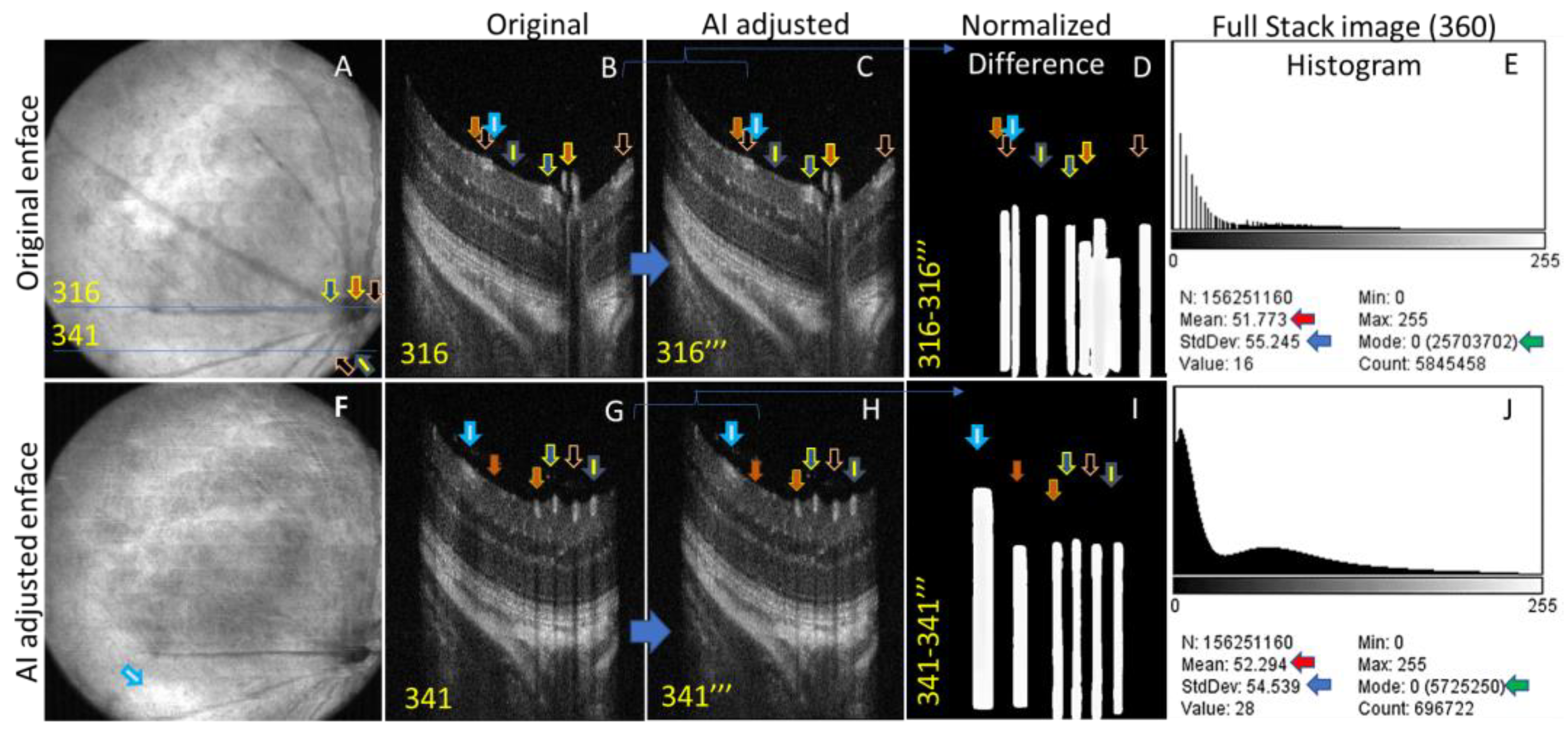
The correlation value between data with and without registration for this data set was 0.703. Once the location of shadows was found, the next step required changing the brightness/pixel gray values. Equation (2) was used to manipulate the pixel value under the shadow only. Sensitivity analysis (a simple brute-force approach) was performed to find the optimized (visual perception was used) value of α = 1.3. The final shadow removed registered (A.I.-adjusted) images, and the respective original images are shown in Figure 7. Figure 7A,B,G show the enface and B scans (index 316 and index 341) of the original data (stack of 360 B scans) and Figure 7C,F,H show the corresponding A.I.-segmented pixel-value-adjusted images for shadow suppression. The effect is visible by comparing Figure 7B with Figure 7C,G and Figure 7H. The shadows, however, were not entirely removed but suppressed. The corresponding normalized differences (with the corresponding shadow locations) are also shown in Figure 7D,I as basically equivalent to the mask created by A.I. to segment these locations. Figure 7B,E show that the chosen value of alpha was able to suppress the existence of relatively thin shadows (highlighted with arrow markers with light blue boundaries and white inner cores) only. The biggest possible dark region right below the optical cord was adjusted as well; however, interpolation to the missing retinal layer maps is not included in this work. The difference between Figure 7B,C is shown in Figure 7D, which depicts the overall changes made by A.I. in this B scan. The major effect of suppressing the shadow was observed in the enface of the full stack of the 360 B scan. The enface of the original images (Figure 7A) suffered the case 2 registration issue and showed dark ILM vessels prominently. The AI-adjusted enface, however, had only a few jitters and dark vessels after post-processing. The histogram data obtained for the respective full stack are shown in Figure 7E,J. The difference in the mean pixel value of shadow-adjusted data increased (1%) from 51.77 to 52.29, and the standard deviation decreased (1.29%) from 55.25 to 54.54. The number of zeros (mode value) decreased (77%) from ${2.57\times 10}^7$ to ${5.73\times 10}^6$. This is reflected in the increased smoothness of the histogram curve. The data set using several values of α was found to have poor performance as far as loss in standard deviation, zero-valued pixels, and increment in mean pixel value are concerned. The positive mean pixel values, negative standard deviation, and the number of zeros can be used as optimization factors to estimate the optimal α rather than using brute-force sensitivity analysis.

3.4. A.I.-Based Retinal Layer Thickness Estimation

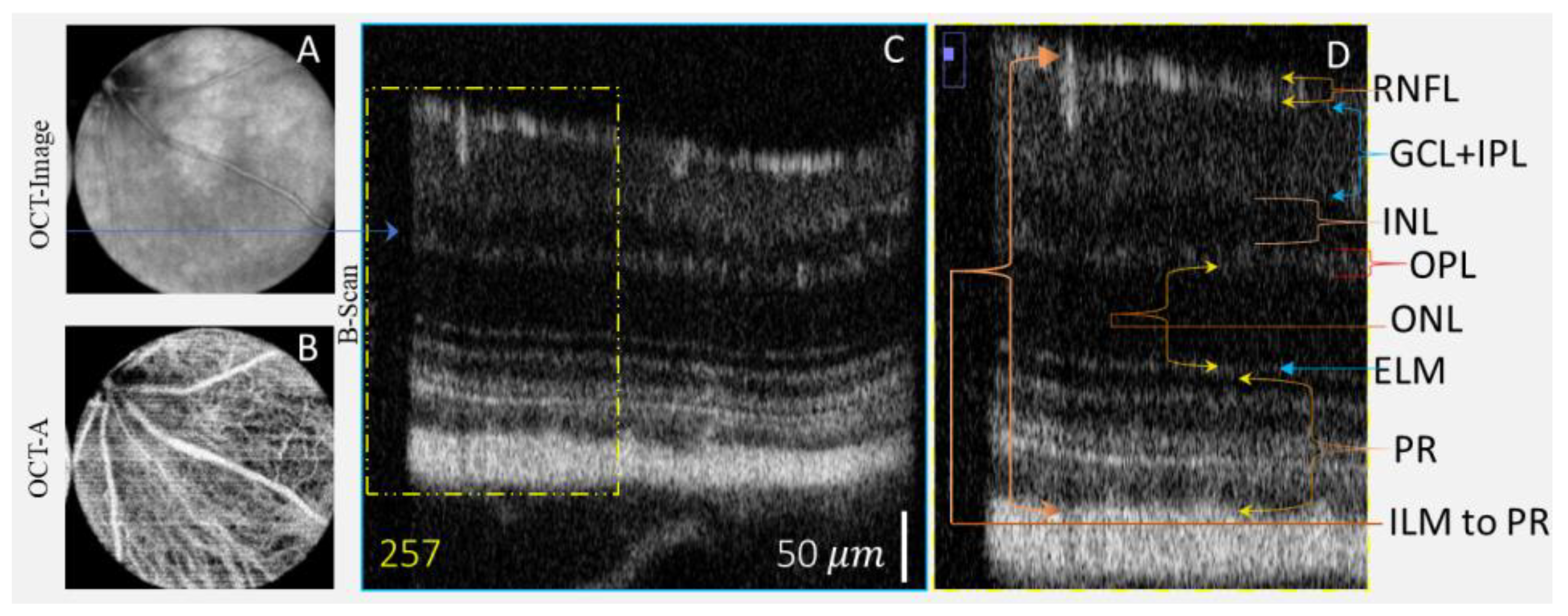
The flow chart of the algorithm is shown in supplementary Figure S2. The implementation of U-Net and its associated parameters is explained elsewhere [24]. The in-vivo imaging session was performed on twenty mice. The OCT B scans and OCT-A enface images were post-processed. Figure 8 shows the retinal layer thickness automatically estimated using an AI-based app. BALB/c female mouse data were used to verify the difference with published data. Enface OCT and its phase variance images are shown in Figure 8A,B. The B scan (as an example) is shown in Figure 8C. Its zoomed version in Figure 8D was used to depict the respective retinal layers along with pixels and lengths in micrometers. It appears that the A.I.-pipeline-generated data were closer to the manually segmented reported data than other tools for this B scan [33]. Supplementary Figure S3 comparatively depicts the binary mask created using U-Net and A.I.-Pipeline and justifies the improvement.

The details are given in

Table 1. Retinal thickness estimation comparison for BalBc female mice.

Layer	Pixels	Thickness Estimated Using AI	Reported Thickness [33]
RNFL	20	16.72	19.32
GCL + IPL	53	44.31	45.09
INL + OPL	25 + 21	20.9 + 17.5 = 38.4	41.92
ONL	52	43.47	46.09
ELM	12	10.03
PR	81	67.72	59.86
ILM to PR	251	209.20	209.20

. The reported thickness from ILM until the end of PR was 209 mm. Sex is not mentioned in this work. The A.I.-segmented average distance (for all B scans using more than 20 mice) in pixels was found to be 251 pixels. This indicates that the axial resolution of the system was 0.836 microns per pixel. The overall estimation had a 6% error.

4. Conclusions

OCT and OCT-A images were obtained from a compact table-top multi-spectral imaging system that was developed in-house. The work presented the AI-based post-processing add-ons required for accurate retinal layer segmentation, especially the suppression of shadows beneath the thicker ILM structures. It was shown that the classical keypoint detection methods, conventional neural network, and A.I. model for medical imaging underperformed for the speckled, noise-ridden mouse eye OCT data when it comes to segmenting low-contrast regions. Tweaking the A.I. model by inserting the batch normalization process provided an acceptable loss value. The retinal thickness estimation accuracy was 94% when 359 images were used for training. The method has limitations, as performance severely depends on the variation available in the training dataset. A healthy animal has relatively fewer morphological variabilities in OCT data than an animal suffering from any disease. Segmented data with and without A.I. post-processing have a difference, as the lack of post-processing gaps in single retinal topography affects the overall estimation. Post-processing was added as an initial step in the layer segmentation pipeline. The customized code was converted into a user-friendly app that allows the user to add their annotated data set for training purposes.

References

1. Fercher, A.F. Optical Coherence Tomography—Development, Principles, Applications. Z. Med. Phys. 2010, 20, 251–276. [Google Scholar] [CrossRef] [PubMed]
2. Augustin, A.J.; Atorf, J. The Value of Optical Coherence Tomography Angiography (OCT-A) in Neurological Diseases. Diagnostics 2022, 12, 468. [Google Scholar] [CrossRef] [PubMed]
3. Welzel, J.; Lankenau, E.; Birngruber, R.; Engelhardt, R. Optical Coherence Tomography of the Human Skin. J. Am. Acad. Dermatol. 1997, 37, 958–963. [Google Scholar] [CrossRef] [PubMed]
4. Spînu, M.; Onea, L.H.; Homorodean, C.; Olinic, M.; Ober, M.C.; Olinic, D.M. Optical Coherence Tomography—OCT for Characterization of Non-Atherosclerotic Coronary Lesions in Acute Coronary Syndromes. J. Clin. Med. 2022, 11, 265. [Google Scholar] [PubMed]
5. Meleppat, R.K.; Ronning, K.E.; Karlen, S.J.; Burns, M.E.; Pugh, E.N.; Zawadzki, R.J. In Vivo Multimodal Retinal Imaging of Disease-Related Pigmentary Changes in Retinal Pigment Epithelium. Sci. Rep. 2021, 11, 16252. [Google Scholar] [CrossRef]
6. Meleppat, R.K.; Ronning, K.E.; Karlen, S.J.; Kothandath, K.K.; Burns, M.E.; Pugh, E.N., Jr.; Zawadzki, R.J. In Situ Morphologic and Spectral Characterization of Retinal Pigment Epithelium Organelles in Mice Using Multicolor Confocal Fluorescence Imaging. Investig. Ophthalmol. Vis. Sci. 2020, 61, 1. [Google Scholar] [CrossRef]
7. Goswami, M.; Wang, X.; Zhang, P.; Xiao, W.; Karlen, S.J.; Li, Y.; Zawadzki, R.J.; Burns, M.E.; Lam, K.S.; Pugh, E.N. Novel Window for Cancer Nanotheranostics: Non-Invasive Ocular Assessments of Tumor Growth and Nanotherapeutic Treatment Efficacy in Vivo. Biomed. Opt. Express 2019, 10, 151–166. [Google Scholar] [CrossRef]
8. Smith, C.A.; Hooper, M.L.; Chauhan, B.C. Optical Coherence Tomography Angiography in Mice: Quantitative Analysis After Experimental Models of Retinal Damage. Investig. Ophthalmol. Vis. Sci. 2019, 60, 1556–1565. [Google Scholar] [CrossRef] [Green Version]
9. Hormel, T.T.; Jia, Y.; Jian, Y.; Hwang, T.S.; Bailey, S.T.; Pennesi, M.E.; Wilson, D.J.; Morrison, J.C.; Huang, D. Plexus-Specific Retinal Vascular Anatomy and Pathologies as Seen by Projection-Resolved Optical Coherence Tomographic Angiography. Prog. Retin. Eye Res. 2021, 80, 100878. [Google Scholar] [CrossRef]
10. Hitzenberger, C.K.; Augustin, M.; Wartak, A.; Baumann, B.; Merkle, C.W.; Pircher, M.; Leitgeb, R.A. Signal Averaging Improves Signal-to-Noise in OCT Images: But Which Approach Works Best, and When? Biomed. Opt. Express 2019, 10, 5755–5775. [Google Scholar] [CrossRef]
11. Jian, Y.; Wong, K.; Sarunic, M.V. Graphics Processing Unit Accelerated Optical Coherence Tomography Processing at Megahertz Axial Scan Rate and High Resolution Video Rate Volumetric Rendering. J. Biomed. Opt. 2013, 18, 026002. [Google Scholar] [CrossRef] [PubMed] [Green Version]
12. Luo, S.; Holland, G.; Mikula, E.; Bradford, S.; Khazaeinezhad, R.; Jester, J.V.; Juhasz, T. Dispersion Compensation for Spectral Domain Optical Coherence Tomography by Time-Frequency Analysis and Iterative Optimization. Opt. Continuum. 2022, 1, 1117–1136. [Google Scholar] [CrossRef]
13. Ni, G.; Zhang, J.; Liu, L.; Wang, X.; Du, X.; Liu, J.; Liu, Y. Detection and Compensation of Dispersion Mismatch for Frequency-Domain Optical Coherence Tomography Based on A-Scan’s Spectrogram. Opt. Express 2020, 28, 19229–19241. [Google Scholar] [CrossRef] [PubMed]
14. Borkovkina, S.; Camino, A.; Janpongsri, W.; Sarunic, M.V.; Jian, Y. Real-Time Retinal Layer Segmentation of OCT Volumes with GPU Accelerated Inferencing Using a Compressed, Low-Latency Neural Network. Biomed. Opt. Express 2020, 11, 3968–3984. [Google Scholar] [CrossRef]
15. Camino, A.; Jia, Y.; Yu, J.; Wang, J.; Liu, L.; Huang, D. Automated Detection of Shadow Artifacts in Optical Coherence Tomography Angiography. Biomed. Opt. Express 2019, 10, 1514–1531. [Google Scholar] [CrossRef]
16. Vladusich, T.; Lucassen, M.P.; Cornelissen, F.W. Brightness and Darkness as Perceptual Dimensions. PLoS Comput. Biol. 2007, 3, 1849–1858. [Google Scholar] [CrossRef] [Green Version]
17. Blakeslee, B.; McCourt, M.E. A Unified Theory of Brightness Contrast and Assimilation Incorporating Oriented Multiscale Spatial Filtering and Contrast Normalization. Vis. Res. 2004, 44, 2483–2503. [Google Scholar] [CrossRef] [Green Version]
18. Wang, J.; Hormel, T.T.; You, Q.; Guo, Y.; Wang, X.; Chen, L.; Hwang, T.S.; Jia, Y. Robust non-perfusion area detection in three retinal plexuses using convolutional neural network in OCT angiography. Biomed. Opt. Express 2020, 11, 330–345. [Google Scholar] [CrossRef]
19. Wang, R.K.; Jacques, S.L.; Ma, Z.; Hurst, S.; Hanson, S.R.; Gruber, A.; Makita, S.; Jaillon, F.; Yamanari, M.; Miura, M.; et al. Projection-Resolved Optical Coherence Tomographic Angiography. Biomed. Opt. Express 2016, 7, 816–828. [Google Scholar] [CrossRef] [Green Version]
20. US20180182082 Systems and Methods for Reflectance-Based Projection-Resolved Optical Coherence Tomography Angiography. Available online: https://patentscope.wipo.int/search/en/detail.jsf?docId=US223549933&recNum=13&docAn=15852521&queryString=(FP/%22Optical%20Coherence%20Tomography%22)%20&maxRec=3853 (accessed on 6 February 2023).
21. Zawadzki, R.J.; Fuller, A.R.; Wiley, D.F.; Hamann, B.; Choi, S.S.; Werner, J.S. Adaptation of a Support Vector Machine Algorithm for Segmentation and Visualization of Retinal Structures in Volumetric Optical Coherence Tomography Data Sets. J. Biomed. Opt. 2007, 12, 41206. [Google Scholar] [CrossRef]
22. Sonobe, T.; Tabuchi, H.; Ohsugi, H.; Masumoto, H.; Ishitobi, N.; Morita, S.; Enno, H.; Nagasato, D. Comparison between Support Vector Machine and Deep Learning, Machine-Learning Technologies for Detecting Epiretinal Membrane Using 3D-OCT. Int. Ophthalmol. 2019, 39, 1871–1877. [Google Scholar] [CrossRef]
23. Zhang, L.; Dong, R.; Zawadzki, R.J.; Zhang, P. Volumetric Data Analysis Enabled Spatially Resolved Optoretinogram to Measure the Functional Signals in the Living Retina. J. Biophotonics 2022, 15, e202100252. [Google Scholar] [CrossRef]
24. Goswami, M. Deep Learning Models for Benign and Malign Ocular Tumor Growth Estimation. Comput. Med. Imaging Graph. 2021, 93, 101986. [Google Scholar] [CrossRef]
25. He, Y.; Carass, A.; Liu, Y.; Jedynak, B.M.; Solomon, S.D.; Saidha, S.; Calabresi, P.A.; Prince, J.L. Structured Layer Surface Segmentation for Retina OCT Using Fully Convolutional Regression Networks. Med. Image Anal. 2021, 68, 101856. [Google Scholar] [CrossRef]
26. Tao, Y.; Ling, Z. Deep Features Homography Transformation Fusion Network—A Universal Foreground Segmentation Algorithm for PTZ Cameras and a Comparative Study. Sensors 2020, 20, 3420. [Google Scholar] [CrossRef] [PubMed]
27. Wei, S.; Kang, J.U. Optical Flow Optical Coherence Tomography for Determining Accurate Velocity Fields. Opt. Express 2020, 28, 25502–25527. [Google Scholar] [CrossRef] [PubMed]
28. SIFT—Scale-Invariant Feature Transform. Available online: http://weitz.de/sift/ (accessed on 24 December 2022).
29. Redmon, J.; Divvala, S.; Girshick, R.; Farhadi, A. You Only Look Once: Unified, Real-Time Object Detection. In Proceedings of the IEEE Computer Society Conference on Computer Vision and Pattern Recognition, Las Vegas, NV, USA, 27–30 June 2016; pp. 779–788. [Google Scholar] [CrossRef] [Green Version]
30. Shakya, S.; Kumar, S.; Goswami, M. Deep Learning Algorithm for Satellite Imaging Based Cyclone Detection. IEEE J. Sel. Top. Appl. Earth Obs. Remote Sens. 2020, 13, 827–839. [Google Scholar] [CrossRef]
31. He, K.; Gkioxari, G.; Dollár, P.; Girshick, R. Mask R-CNN. IEEE Trans. Pattern Anal. Mach. Intell. 2017, 42, 386–397. [Google Scholar] [CrossRef] [PubMed]
32. Viedma, I.A.; Alonso-Caneiro, D.; Read, S.A.; Collins, M.J. OCT Retinal and Choroidal Layer Instance Segmentation Using Mask R-CNN. Sensors 2022, 22, 2016. [Google Scholar] [CrossRef]
33. Dysli, C.; Enzmann, V.; Sznitman, R.; Zinkernagel, M.S. Quantitative Analysis of Mouse Retinal Layers Using Automated Segmentation of Spectral Domain Optical Coherence Tomography Images. Transl. Vis. Sci. Technol. 2015, 4, 9. [Google Scholar] [CrossRef] [Green Version]
Figure 1. Image registration benefits and issues with inaccuracies: (AC) show three successive B scans with a slight decrease in height from the top of the time, with the respective SNR and zoomed part showing ELM and RPE in the inset; (D) shows the averaged B Scan of (AC) without registration, showing that SNR is improved but fake retinal layers appear.
Photonics 10 00275 g001
Figure 2. The effect of suboptimal dispersion correction parameters; Figure (AI) shows the effect of mouse eye movement as the retinal layer depiction sharpness is affected, starting from (B) and ending at (H), (I) shows false depiction of breakage in perfectly healthy vessel, (J) is enface of full stack and (K) is B Scan showing optical chord.
Photonics 10 00275 g002
Figure 3. Output of algorithms for image registration. (A) Sample image A is the image that needs registration, (BD) shows the keypoints obtained from mapping between the reference image and sample image (after registration) obtained by SIFT, ORB, and a combination of ORB and BEBILD, respectively. (E) shows the registered image using optical flow. The correlation value remained below 0.6 for all.
Photonics 10 00275 g003
Figure 4. Registration using deep CNN: (A) in-house developed CNN model architecture, (B) loss values vs. epochs, (C) initial model parameter details, (D,E) annotation models, (FH) are, sample, and registered images.
Photonics 10 00275 g004
Figure 5. Classical approaches for shadow removal, (A) highlights the presence of shadow artifacts in sample image, (B) after convolving the same image using filter, (C) when sample image is averages using zero axis rolling technique, (D) HSV tweaking results are better than (E) when sample image is applied with adjacent column dependent averaging and (F) blurred.
Photonics 10 00275 g005
Figure 6. AI-based segmentation of the region under the shadows. (A) sample image showing shadow artifact, (B) and (C) show the annotation locations overlapped with sample images performed at U-Net and R-CNN and their respective mask are shown in (D) and (E).
Photonics 10 00275 g006
Figure 7. A.I.-segmented pixel-value-adjusted images for shadow suppression: (A) enface image without shadow suppression, (B) B scans corresponding to blue horizontal lines in (A) with index 316, (C) B Scan after suppressing the shadow artifacts corresponding to (B), (D) is the normalized difference between original image (B) and image (C), (E) Histogram of full stack (360 B scans) without shadow suppression (F) enface after AI-based shadow suppression, (G) B scans corresponding to blue horizontal lines in (A) with index 341, (H) B Scan after shadow suppression, (I) difference between images shown in (G,H), (J) is the Histogram of full stack (360 B scans) after shadow suppression.
Photonics 10 00275 g007
Figure 8. AI-based automatic retinal layer thickness estimation of BalBc female mice; (A,B) enface OCT and phase variance images, (C) the B scan with 257 indices (marked in the OCT image with a blue line), and (D) the zoomed section from an earlier image with the retinal layers/sections segmented.
Photonics 10 00275 g008