A Comparison of the Robust Zero-Inflated and Hurdle Models with an Application to Maternal Mortality

Abstract

This study evaluates the performance of count regression models in the presence of zero inflation, outliers, and overdispersion using both simulated and real-world maternal mortality dataset. Traditional Poisson and negative binomial regression models often struggle to account for the complexities introduced by excess zeros and outliers. To address these limitations, this study compares the performance of robust zero-inflated (RZI) and robust hurdle (RH) models against conventional models using the Akaike Information Criterion (AIC) and Bayesian Information Criterion (BIC) to determine the best-fitting model. Results indicate that the robust zero-inflated Poisson (RZIP) model performs best overall. The simulation study considers various scenarios, including different levels of zero inflation (50%, 70%, and 80%), outlier proportions (0%, 5%, 10%, and 15%), dispersion values (1, 3, and 5), and sample sizes (50, 200, and 500). Based on AIC comparisons, the robust zero-inflated Poisson (RZIP) and robust hurdle Poisson (RHP) models demonstrate superior performance when outliers are absent or limited to 5%, particularly when dispersion is low (5). However, as outlier levels and dispersion increase, the robust zero-inflated negative binomial (RZINB) and robust hurdle negative binomial (RHNB) models outperform robust zero-inflated Poisson (RZIP) and robust hurdle Poisson (RHP) across all levels of zero inflation and sample sizes considered in the study.

1. Introduction

Excess zeros are common in numerous fields, including healthcare, agriculture, ecology, and manufacturing industries [1,2]. A Zero-Inflated (ZI) model [3] argues that zero counts arise from a combination of two distributions; one distribution generates structural zeros, representing subjects who are not at all at risk of experiencing the event (and thus consistently produce zero counts). For instance, when quantifying specific high-risk behaviors, certain individuals may record a score of zero due to their lack of susceptibility to such health-risk behaviors [4]. The second distribution generates sampling zeros, representing individuals who are at risk but did not experience or report the event during the study period. The justification for categorizing zeros into two categories is that a high proportion of zeros frequently results from the presence of a subgroup of patients who are not at risk for certain outcomes during the study period [3]. The probability of belonging to the zero inflation component is assessed using a Bernoulli model, while a standard count distribution, such as Poisson or negative binomial (NB), represents the counts in the count component [5]. Conversely, a hurdle model [6] claims that all zero observations originate from a singular structural source, comprising a binary component to determine whether the response variable is zero or positive, alongside a truncated model, such as a truncated Poisson or truncated NB distribution, for the positive data. Excess zeros indicate more zeros than the distribution we are modeling would expect. Zero-inflated and hurdle models have been used extensively in various research domains to model such data [2,7]. The traditional models, such as the standard Poisson and NB models, often fail to address the complexity of outliers, overdispersion, and excess zeros simultaneously. The understanding and useful comparison of the robust zero-inflated (RZI) and robust hurdle (RH) models remain largely unexplored, despite substantial advances in statistical modeling methods for count data [1,2]. Although both models address the frequent excess zeros seen in the count data, their fundamental tenets and estimating strategies are different.

Maternal mortality data often exhibit zero inflation, characterized by an excess of zero counts or units reporting no maternal deaths, compared to what standard count models such as Poisson or NB would predict [8,9]. Identifying factors that contribute to maternal mortality and formulating effective interventions are essential to minimize the increase in maternal mortality. In this context, there is a need to employ statistical models that can adequately handle the excessive zeros, overdispersion, and potential outliers that are often observed in maternal mortality [10]. Previous studies that have looked at factors affecting maternal death have used different analysis strategies, with some ignoring the underlying zero inflation [11,12]. There has been considerable interest in the literature in comparing zero-inflated and hurdle models for analyzing count data with excess zeros and outliers [2,10,13]. However, the robustness to outliers that these comparisons frequently neglect can have significant effects on the accuracy and reliability of the models’ results. Robust zero-inflated models and robust hurdle models have been proposed to handle outliers in addition to zero inflation. There is a lack of comprehensive studies that directly examine the performance of robust hurdle and zero-inflated models in the presence of outliers. In addition, there has been little research on the application of these models to maternal mortality data [1,2,12], an important public health indicator. Using simulated data and data on maternal mortality, this study attempts to close these gaps by comparing the robust zero-inflated and hurdle models in the presence of outliers. Through this investigation, the study hopes to shed light on how well these models handle excessive zeros and outliers in count data, with an emphasis on enhancing modeling accuracy and forecasting rates of maternal death.

2. Methods

2.1. Overview of Count Data Models

This section outlines the statistical frameworks employed to model count data, addressing key challenges such as zero inflation, overdispersion, and outliers. Introduces robust extensions of conventional models, specifically robust zero-inflated and hurdle models, which are designed to improve estimation accuracy in the presence of deviations from model assumptions and outliers. These robust models provide a more reliable analytical framework for real-world datasets, particularly in maternal mortality research, where data irregularities are common.

2.2. Classical Zero-Inflated and Hurdle Models

2.2.1. Standard Zero-Inflated (ZI) Models

In the ZI model introduced by [3], zero outcomes can originate from two distinct sources. We have structural zeros, which occur due to an inherent process, and sampling zeros, which arise from a standard count distribution such as Poisson or NB. The general form of a ZI model is as follows:

$$P(Y_i=y_i)=\left\{\begin{array}{cc}{\pi }_i+(1-{\pi }_i)p(y_i=0;{\mu }_i)\hfill & \mathrm{if}{y}_i=0,\hfill \\ (1-{\pi }_i)p(y_i;{\mu }_i)\hfill & \mathrm{if}{y}_i>0,\hfill \end{array}\right.$$

(1)

which combines a degenerate distribution at zero and an untruncated count distribution parameterized by ${\mu }_i$. When the count component follows a Poisson distribution, the model becomes a Zero-Inflated Poisson (ZIP) model:

$$P(Y_i=y_i)=\left\{\begin{array}{cc}{\pi }_i+(1-{\pi }_i)e^{-{\mu }_i}\hfill & \mathrm{if}{y}_i=0,\hfill \\ (1-{\pi }_i){\displaystyle \frac{e^{-{\mu }_i}{\mu }_i^{y_i}}{y_i!}}\hfill & \mathrm{if}{y}_i>0,\hfill \end{array}\right.$$

(2)

here, ${\mu }_i$ is the Poisson mean and ${\pi }_i$ is the probability of structural zeros. The mean and variance of the ZIP model are then given by the following:

$$\begin{array}{cc}\hfill \mathbb{E}\left(Y_i\right)& =\mathbb{E}\left[\mathbb{E}\left(y_i\right|z_i)\right]=(1-{\pi }_i){\mu }_i,\hfill \end{array}$$

(3)

$$\begin{array}{cc}\hfill \mathrm{Var}\left(Y_i\right)& =\mathbb{E}\left[Var\left(y_i\right|z_i)\right]+Var\left[\mathbb{E}\left(y_i\right|z_i)\right]=(1-{\pi }_i){\mu }_i(1+{\pi }_i{\mu }_i).\hfill \end{array}$$

(4)

To model the count part of a zero inflation, Poisson regression assumes that the mean and variance are equal. However, real-world data often show overdispersion, where the variance exceeds the mean. This may result from unobserved heterogeneity, omitted variables, clustering, or outliers [14,15]. In such cases, the NB model is more appropriate. The ZINB model, which accounts for both excess zeros and overdispersion, is specified as

$$P(Y_i=y_i)=\left\{\begin{array}{cc}{\pi }_i+(1-{\pi }_i){\left({\displaystyle \frac{r}{{\mu }_i+r}}\right)}^r\hfill & \mathrm{if}{y}_i=0,\hfill \\ (1-{\pi }_i){\displaystyle \frac{\mathrm{\Gamma }(y_i+r)}{\mathrm{\Gamma }\left(r\right)y_i!}}{\left({\displaystyle \frac{{\mu }_i}{{\mu }_i+r}}\right)}^{y_i}{\left({\displaystyle \frac{r}{{\mu }_i+r}}\right)}^r\hfill & \mathrm{if}{y}_i>0,\hfill \end{array}\right.$$

(5)

where ${\mu }_i$ is the NB mean, ${\pi }_i$ is the structural zero probability, r is the dispersion parameter, and $\mathrm{\Gamma }$ is the gamma function. The mean and variance are as follows:

$$\begin{array}{cc}\hfill \mathbb{E}\left(Y_i\right)& =(1-{\pi }_i){\mu }_i,\hfill \end{array}$$

(6)

$$\begin{array}{cc}\hfill \mathrm{Var}\left(Y_i\right)& =(1-{\pi }_i){\mu }_i\left(1+{\displaystyle \frac{{\mu }_i}{r}}+{\pi }_i{\mu }_i\right).\hfill \end{array}$$

(7)

As $r\to \infty$, the ZINB model converges to the ZIP model. Smaller values of r indicate higher overdispersion. In practical applications, both ${\mu }_i$ and ${\pi }_i$ are modeled using explanatory variables. The ZI models can thus be parameterized as

$$log\left({\mu }_i\right)={\mathit{x}}_{\mathit{i}}^{\top }\mathit{\beta },\mathrm{logit}\left({\pi }_i\right)={\mathit{z}}_{\mathit{i}}^{\top }\mathit{\alpha },$$

(8)

where ${\mathit{x}}_{\mathit{i}}$ and ${\mathit{z}}_{\mathit{i}}$ are covariate vectors for the count and zero components, respectively, and $\mathit{\alpha }$ and $\mathit{\beta }$ are their corresponding coefficients. The covariates for ${\mu }_i$ and ${\pi }_i$ need not be the same.

2.2.2. Standard Hurdle Models

As an alternative to ZI models, hurdle models [6] are formulated as two component mixture models. They consist of a component that models excess zeros and another that models positive counts using a truncated count distribution, such as the truncated Poisson or truncated NB distribution. Let $Y_i$ denote the count response for the i-th observation, where $i=1,\dots ,n$, and n is the total number of observations. The general form of a hurdle model is expressed as

$$P(Y_i=y_i)=\left\{\begin{array}{cc}{\pi }_i\hfill & \mathrm{if}{y}_i=0,\hfill \\ (1-{\pi }_i){\displaystyle \frac{p(y_i;{\mu }_i)}{1-p(0;{\mu }_i)}}\hfill & \mathrm{if}{y}_i>0,\hfill \end{array}\right.$$

(9)

where ${\pi }_i$ is the probability of observing a structural zero, and $p(y_i;{\mu }_i)$ is the probability mass function (PMF) of a standard count distribution parameterized by vector ${\mu }_i$. The denominator, $1-p(0;{\mu }_i)$, normalizes the distribution to reflect that only positive counts are considered. If the count component follows a Poisson distribution, the corresponding hurdle Poisson model is

$$P(Y_i=y_i)=\left\{\begin{array}{cc}{\pi }_i\hfill & \mathrm{if}{y}_i=0,\hfill \\ (1-{\pi }_i){\displaystyle \frac{e^{-{\mu }_i}{\mu }_i^{y_i}/y_i!}{1-e^{-{\mu }_i}}}\hfill & \mathrm{if}{y}_i>0.\hfill \end{array}\right.$$

(10)

where the ${\pi }_i$ denotes the probability of a zero count, ${\mu }_i$ is the mean of the underlying Poisson distribution. The mean and variance of the HP are then given by

$$\mathbb{E}\left(Y\right)=(1-\pi )·{\displaystyle \frac{\mu }{1-e^{-\mu }}}$$

(11)

$$\mathrm{Var}\left(Y\right)=(1-\pi )\left[{\displaystyle \frac{\mu (1+\mu e^{-\mu })}{{(1-e^{-\mu })}^2}}+\pi {\left({\displaystyle \frac{\mu }{1-e^{-\mu }}}\right)}^2\right],$$

(12)

to handle overdispersion in count data, the positive count component can alternatively follow an NB distribution. The HNB model is then given by

$$P(Y_i=y_i)=\left\{\begin{array}{cc}{\pi }_i\hfill & \mathrm{if}{y}_i=0,\hfill \\ {\displaystyle \frac{1-{\pi }_i}{1-{\left({\displaystyle \frac{r}{{\mu }_i+r}}\right)}^r}}·{\displaystyle \frac{\mathrm{\Gamma }(y_i+r)}{\mathrm{\Gamma }\left(r\right)y_i!}}{\left({\displaystyle \frac{{\mu }_i}{{\mu }_i+r}}\right)}^{y_i}{\left({\displaystyle \frac{r}{{\mu }_i+r}}\right)}^r\hfill & \mathrm{if}{y}_i>0,\hfill \end{array}\right.$$

(13)

where r is the dispersion parameter and ${\mu }_i$ is the mean of the NB distribution, is the $\mathrm{\Gamma }$ is the gamma function, and ${\pi }_i$ is the structural zero probability. The mean and variance of the HNB model are given by

$$\mathbb{E}\left(Y\right)=(1-{\pi }_i)·{\displaystyle \frac{\mu }{1-{\left(\frac{r}{\mu +r}\right)}^r}},$$

(14)

$$\mathrm{Var}\left(Y_i\right)=(1-{\pi }_i)·{\displaystyle \frac{{\mu }_i+\frac{{\mu }_i^2}{r}}{1-{\left(\frac{r}{r+{\mu }_i}\right)}^r}}+{\pi }_i(1-{\pi }_i){\left({\displaystyle \frac{{\mu }_i}{1-{\left(\frac{r}{r+{\mu }_i}\right)}^r}}\right)}^2.$$

(15)

As with ZI models, covariates can be incorporated into both the zero and count components. The hurdle model can thus be parameterized as

$$log\left({\mu }_i\right)={\mathit{x}}_{\mathit{i}}^{\top }\mathit{\beta },\mathrm{logit}\left({\pi }_i\right)={\mathit{z}}_{\mathit{i}}^{\top }\mathit{\alpha },$$

(16)

where $\mathit{\alpha }$ and $\mathit{\beta }$ are vectors of regression coefficients for the covariates ${\mathit{x}}_{\mathit{i}}$ and ${\mathit{z}}_{\mathit{i}}$, respectively.

2.3. Robust Extensions of Zero-Inflated and Hurdle Models

2.3.1. Robust Zero-Inflated Models

Although ZIP and ZINB models handle excess zeros, they can be sensitive to outliers. The RZIP and RZINB models improve the standard ZI models by incorporating robust estimation techniques. The robust zero-inflated models (RZIP and RZINB), first proposed by [5] and later refined by [16], integrate Huber’s M-estimation into standard ZIP/ZINB structures. The robust approach uses the Huber $\mathrm{\Psi }$-function [17], to downweight extreme values during parameter estimation. In the RZI models, the parameters are estimated using a robust Expectation–Maximization (EM) algorithm by [5]. In mixture models like ZI, the EM algorithm is a natural approach for computing maximum likelihood estimates (MLEs) [3]. This algorithm works by introducing latent variables that indicate whether a zero outcome came from the excess zero component or from the count distribution. According to [5] we define ${\tau }_i=1$ when the observation $y_i$ originates from the zero inflation component, and ${\tau }_i=0$ for the non-zero state

$${\tau }_i=\left\{\begin{array}{cc}1\hfill & \mathrm{if}{y}_i\mathrm{is}\mathrm{from}\mathrm{the}\mathrm{zero}\mathrm{state},\hfill \\ 0\hfill & \mathrm{if}{y}_i\mathrm{is}\mathrm{from}\mathrm{the}\mathrm{non}-\mathrm{zero}\mathrm{state}.\hfill \end{array}\right.$$

With this, the complete data log-likelihood can be expressed as

$${\mathit{\ell }}^c(\mathit{\alpha },\mathit{\beta };\mathit{y},\mathit{\tau })=\sum _{i=1}^n\left\{{\tau }_i{\mathit{z}}_{\mathit{i}}^{\top }\mathit{\alpha }-log(1+e^{{\mathit{z}}_{\mathit{i}}^{\top }\mathit{\alpha }})\right\}+\sum _{i=1}^n(1-{\tau }_i)logf({\mathit{y}}_{\mathit{i}};{\mathit{x}}_{\mathit{i}}^{\top }\mathit{\beta }),$$

(17)

where ${\mathit{\tau }}_{\mathit{i}}={({\tau }_1,\dots ,{\tau }_n)}^{\top }$. Maximizing this log-likelihood is straightforward because the complete data log-likelihood functions for $\mathit{\alpha }$ and $\mathit{\beta }$, denoted by ${\mathit{\ell }}_{\alpha }^c(\mathit{\alpha };\mathit{y},\mathit{\tau })$ and ${\mathit{\ell }}_{\beta }^c(\mathit{\beta };\mathit{y},\mathit{\tau })$, can be optimized separately with respect to their respective parameters using standard methods. The EM algorithm maximizes the log-likelihood of models (10) and (13) through an iterative process consisting of two main steps which is the E-step and the M-step. In the E-step, each latent variable $z_i$ is replaced by its conditional expectation, given the current estimates of $(\mathit{\alpha },\mathit{\beta })$. In the M-step, these expected values are treated as fixed, and the complete data log-likelihood ${\mathit{\ell }}^c(\mathit{\beta },\mathit{\alpha };\mathit{y},\mathit{z})$ is maximized with respect to $\mathit{\alpha }$ and $\mathit{\beta }$. These two steps are repeated alternately until the parameter estimates converge. The algorithm begins with initial values ${\mathit{\theta }}^{\left(0\right)}={({\mathit{\alpha }}^{\left(0\right)\top },{\mathit{\beta }}^{\left(0\right)\top })}^{\top }$ and proceeds iteratively through the following three steps until convergence.

E-step: Estimate ${\tau }_i$ by its conditional expectation ${\tau }_i^t$ given the current estimates ${\mathit{\alpha }}^{\left(r\right)}$ and ${\mathit{\beta }}^{\left(r\right)}.$

$${\tau }_i^{\left(t\right)}={\displaystyle \frac{P(y_i\mid \mathrm{zero}\mathrm{state})P\left(\mathrm{zero}\mathrm{state}\right)}{P(y_i\mid \mathrm{zero}\mathrm{state})P\left(\mathrm{zero}\mathrm{state}\right)+P(y_i\mid \mathrm{non}-\mathrm{zero}\mathrm{state})P\left(\mathrm{non}-\mathrm{zero}\mathrm{state}\right)}}.$$

M-step for $\alpha$. Find ${\alpha }^{(t+1)}$ by maximizing ${\mathit{\ell }}_{\alpha }^c(\alpha ;y,{\tau }^{\left(t\right)})$, equivalent to solving

$${\displaystyle \frac{1}{n}}\sum _{i=1}^n\left\{{\tau }_i^{\left(t\right)}-{\mathrm{logit}}^{-1}\left({\mathit{z}}_{\mathit{i}}^{\top }\mathit{\alpha }\right)\right\}{\mathit{z}}_{\mathit{i}}=0.$$

(18)

M-step for $\mathit{\beta }$. For the non-degenerate component, we find ${\mathit{\beta }}^{(t+1)}$ by maximizing ${\mathit{\ell }}_{\alpha }^c(\mathit{\alpha };\mathit{y},{\tau }^{\left(t\right)})$ which is equivalent to solving the estimation $\mathit{\beta }$;

$${\displaystyle \frac{1}{n}}\sum _{i=1}^n(1-{\tau }_i^{\left(t\right)})\left\{y_i-e^{{\mathit{x}}_{\mathit{i}}^{\top }\mathit{\beta }}\right\}{\mathit{x}}_{\mathit{i}}=0.$$

(19)

Hall [5] proposed in the RES approach that the estimating functions (18) and (19) from the M-step of the EM algorithm can be achieved with robustified estimating functions. That is, we downweight observations in the extreme tails of the Poisson or NB component using a bounded influence function ${\psi }_c$, and apply leverage-based weights $\omega (·)$. To robustify the estimation, we replace the standard score functions in Equations (18) and (19) with bounded influence versions that combine residual trimming through ${\psi }_c$ and leverage weighting via $\omega (·)$. Specifically, solving for the parameter ${\alpha }^{(t+1)}$ and ${\beta }^{(t+1)}$ in the following Equations (20) and (21). The estimation equation for the zero inflation component parameter $\mathit{\alpha }$ is expressed as follows:

$${\displaystyle \frac{1}{n}}\sum _{i=1}^n\omega \left({\mathit{z}}_{\mathit{i}}\right)\left\{{\tau }_i^{\left(t\right)}-{\mathrm{logit}}^{-1}\left({\mathit{z}}_{\mathit{i}}^{\top }\mathit{\alpha }\right)\right\}{\mathit{z}}_{\mathit{i}}=0,$$

(20)

$${\displaystyle \frac{1}{n}}\sum _{i=1}^n(1-{\tau }_i^{\left(t\right)})\omega \left({\mathit{x}}_{\mathit{i}}\right)\left\{{\psi }_c\left(y_i\right)-o_i(\mathit{\beta },c)\right\}{\mathit{x}}_{\mathit{i}}=0,$$

(21)

where for the non-degenerate Poisson component, $o_i(\mathit{\beta },c)=E\left\{{\psi }_c\left(Y_i\right)|Y_i\sim \mathrm{Poisson}\left({\mu }_i\right)\right\}=j_{1}P(Y_i<j_1)+{\mu }_{i}P(j_1\le Y_i\le j_2)+j_{2}P(Y_i>j_2),$ and for the negative binomial component, $o_i^{\mathrm{NB}}(\mathit{\beta },r,c)=j_{1}P(Y_i<j_1)+E[Y_i\mid j_1\le Y_i\le j_2]·P(j_1\le Y_i\le j_2)+j_{2}P(Y_i>j_2),$ where $Y_i\sim \mathrm{NB}({\mu }_i,r)$. The function ${\psi }_c\left(y\right)$ truncates extreme responses:

$${\psi }_c\left(y\right)=\left\{\begin{array}{cc}{j}_1,\hfill & y<j_1,\hfill \\ y,\hfill & y\in [j_1,j_2],\hfill \\ j_2,\hfill & y>j_2,\hfill \end{array}\right.$$

with $j_1$ and $j_2$ being the c and $(1-c)$ quantiles of the non-degenerate distribution (Poisson or NB). The downweighting function $\omega (·)$ is used to reduce the influence of high-leverage points, and is taken as $\omega \left({\mathit{z}}_{\mathit{i}}\right)=\sqrt{1-h_i}$, where $h_i$ is the leverage from the design matrix ${\mathit{z}}_{\mathit{i}}$, with an analogous definition for ${\mathit{x}}_{\mathit{i}}$.

2.3.2. Robust Hurdle Models

The robust hurdle models used in this study build upon the methodology developed by [18], who proposed a robust version of the hurdle models that are based on standard hurdle models by incorporating bounded influence estimation through the $\mathrm{\Psi }$-Huber function to mitigate the influence of outliers [19]. For the binary hurdle component, we replace the standard logistic regression with a robust logistic regression using the $\mathrm{\Psi }$-Huber function [17]. This ensures that outliers in the binary classification of zeros and non-zeros have less influence.

$$\sum _{i=1}^n\left[{\psi }_c\left(r_i\right)w\left({\mathit{x}}_{\mathit{i}}\right){\displaystyle \frac{1}{\sqrt{v_{{\mu }_i}}}}{\mu }_i^{\prime }-a\left(\mathit{\beta }\right)\right]=\sum _{i=1}^n\psi (y_i,{\mu }_i)=0,$$

(22)

where $r_i=(y_i-{\mu }_i)/\sqrt{v_{{\mu }_i}}$ are the Pearson residuals, $v_{{\mu }_i}=Var\left(Y_i\right|Y_i>0)$ denotes the conditional variance of the positive count component, i.e., the variance of the truncated Poisson or truncated NB distribution, ${\psi }_c\left(r\right)=min(c,max(r,-c))$ is the Huber function, ${\mu }_i^{\prime }=(\partial /\partial \beta ){\mu }_i$, and where

$$a\left(\mathit{\beta }\right)=\int {\psi }_c\left(r\right)w\left(\mathit{x}\right){\displaystyle \frac{1}{\sqrt{v_{{\mu }_i}}}}{\mu }^{\prime }dF\left(y\right|\mathit{x})d{F}_n\left(\mathit{x}\right)={\displaystyle \frac{1}{n}}\sum _{i=1}^{n}E\left[{\psi }_c\left(r_i\right)\right]w\left({\mathit{x}}_{\mathit{i}}\right){\displaystyle \frac{1}{\sqrt{v_{{\mu }_i}}}}{\mu }_i^{\prime },$$

ensures that Fisher is consistent with $\mathit{\beta }$. We have this for the truncated Poisson component

$$E^{\mathrm{trunc}}\left[{\psi }_c\left(r_i\right)\right]={\displaystyle \frac{1}{1-e^{-{\mu }_i}}}\left[c\left(P(Y_i\ge j_2+1)-P(Y_i\le j_1)\right)+{\displaystyle \frac{{\mu }_i}{\sqrt{v_{{\mu }_i}}}}\left(P(Y_i=j_1)-P(Y_i=j_2)\right)\right],$$

(23)

where $Y_i\sim \mathrm{Poisson}\left({\mu }_i\right)$, variance $v_{{\mu }_i}$, and this for the truncated NB component

$$E^{\mathrm{trunc}}\left[{\psi }_c\left(r_i\right)\right]={\displaystyle \frac{1}{1-{\left(\frac{r}{{\mu }_i+r}\right)}^r}}\left[c\left(P(Y_i\ge j_2+1)-P(Y_i\le j_1)\right)+{\displaystyle \frac{{\mu }_i}{\sqrt{v_{{\mu }_i}}}}\left(P(Y_i=j_1)-P(Y_i=j_2)\right)\right],$$

(24)

where $Y_i\sim \mathrm{NB}({\mu }_i,r)$, variance $v_{{\mu }_i}$, and cutoff points

$$j_1=\left[{\mu }_i-c\sqrt{v_{{\mu }_i}}\right],j_2=\left[{\mu }_i+c\sqrt{v_{{\mu }_i}}\right].$$

The classical estimating equations of the quasi-likelihood estimator for GLM imply the structure of (22). These would utilize $\psi (y_i,{\mu }_i)=((y_i-{\mu }_i)/v_{{\mu }_i}){\mu }_i^{\prime }.$ The function ${\psi }_c\left(r_i\right)$ in (22) is responsible for managing deviations in the y-space. To manage deviations in the design space, leverage points are downweighted by adding weights $w\left(x_i\right)$. For instance, $w\left({\mathit{x}}_{\mathit{i}}\right)=\sqrt{1-h_i}$, where $h_i$ is the ith diagonal element of the hat matrix. According to the use in linear regression, the estimator produced from (22) is called a Mallows-type estimator. It reduces to a Huber-type estimator for all i when $w\left({\mathit{x}}_{\mathit{i}}\right)=1$. Note that it is easy to rewrite the estimating equations (22) as

$$\sum _{i=1}^n\left[\tilde{w}\left(r_i\right)w\left({\mathit{x}}_{\mathit{i}}\right){\displaystyle \frac{1}{\sqrt{v_{{\mu }_i}}}}{r}_i{\mu }_i^{\prime }-a\left(\mathit{\beta }\right)\right]=0.$$

(25)

The function $\tilde{w}\left(r_i\right)={\psi }_c\left(r_i\right)/r_i$ reflects the structure of weighted estimating equations involving two types of weights: $\tilde{w}\left(r_i\right)$ applied to the residuals and $w\left({\mathbf{x}}_i\right)$ applied to the design matrix.

2.4. Model Comparison

To assess the performance of the six different models (Poisson, NB, RZIP, RZINB, RHP, and RHNB) under different simulation scenarios, the study adopted the widely used model selection criteria: Akaike’s information criteria (AIC) developed by [20]. AIC has been presented as a model selection criterion for comparing non-nested models based on maximum likelihood, utilizing the fitted log-likelihood function to identify the optimal model. The AIC evaluates the relative quality of a statistical model by rewarding goodness of fit while imposing a penalty that increases with the number of estimated parameters. As the log-likelihood is anticipated to rise with the addition of parameters to a model, the AIC criterion imposes a penalty on models with a greater number of parameters (q). The penalty function may also depend on n, the number of observations. This penalty prevents overfitting. Consequently, the AIC is defined as

$$\mathrm{AIC}=-2log\left(L\right)+2q,$$

where L is the maximal likelihood function value for the estimated model, q is the number of degrees of freedom, and 2 is a tuning parameter to balance the information in the model with the residuals, according to the number of degrees of freedom. It is desirable to choose a model with the lowest AIC. Although AIC penalizes the complexity of the model using a constant factor of 2 per parameter, another widely used criterion, the Bayesian Information Criterion (BIC), takes a different approach. Like AIC, BIC rewards goodness of fit but introduces a stronger penalty for model complexity, which makes BIC more conservative. The Bayesian Information Criterion (BIC) is defined as follows:

$$\mathrm{BIC}=-2log\left(L\right)+klog\left(n\right),$$

where L is the likelihood of the model, k is the number of parameters, and n is the sample size. When fitting models, it is possible to increase the likelihood by adding parameters, but doing so may result in overfitting. The BIC addresses this issue by introducing a penalty term for the number of parameters in the model. The penalty term in BIC is larger than the penalty term in AIC.

3. Simulation Study

To assess the performance of standard and robust count regression models under varying levels of overdispersion, zero inflation, and contamination, a structured simulation study was conducted. The dataset was generated from the ZINB model, which is characterized by a mean variance of this form

$$Var\left(Y_i\right)={\mu }_i(1+{\displaystyle \frac{{\mu }_i}{r}}),$$

(26)

that allows the variance to be greater than the mean, a common choice for modeling overdispersed count data such as maternal mortality in this study. The simulation design considered combinations of four key factors which are sample size (50, 200, and 500), dispersion levels $(r=1,3,5)$, i.e., 1 is considered as high dispersion, 3 as moderate, and 5 as low in this study, structural zero proportions (0.5, 0.7, and 0.8), and outlier proportions (0.00, 0.05, 0.10, and 0.15). A summary of the simulation scenarios considered in the study is shown below in

Table 1. Simulation scenarios considered in the simulation study.

Sample Size	Prop of Zeros	Dispersion	Outliers
			0.00
50	0.5	1	0.05
200	0.7	3	0.10
500	0.8	5	0.15

. This produced 3 × 3 × 3 × 4 = 108 distinct simulation scenarios in all. Each scenario was run 1000 times to reduce the influence of simulation error, and the AIC was averaged over the 1000 runs.

For each observation $i=1,\dots ,n$, the response variable was generated from the ZINB model:

$$Y_i\sim \mathrm{ZINB}({\pi }_i,{\mu }_i,r),$$

$$Y_i=\left\{\begin{array}{c}{\pi }_i+(1-{\pi }_i)·P_{\mathrm{NB}}\left(0\right|{\mu }_i,r)y_i=0\hfill \\ (1-{\pi }_i)·P_{\mathrm{NB}}\left(y\right|{\mu }_i,r)y_i>0\hfill \end{array}\right.$$

with the mean ${\mu }_i$, ${\pi }_i$ is the structural zero probability, and dispersion r where $log\left({\mu }_i\right)=x_i·\alpha$ with a single continuous covariate $x_i$ drawn independently from a uniform distribution $x_i\sim \mathrm{Uniform}(0,1)$. The intercept was fixed at 1, and the slope coefficient at 1.5, where $x_i=(1,x_i)$ and $\alpha ={(1,1.5)}^T.$ To assess the robustness of the models to extreme values, outliers were introduced in the simulated data by randomly selecting a proportion of the observations determined by the specified outlier level (0, 0.05, 0.10, or 0.15), and inflating their outcome values by a factor of 10. Specifically, for a given sample size n, a total of $\left[n\times \mathit{outlier}\mathit{level}\right]$ indices were randomly sampled, and the corresponding response values were multiplied by 10. This approach simulates extreme count values that may arise due to data entry errors or rare events, allowing us to evaluate the model’s performance in the presence of such anomalies.

3.1. Simulation Study Findings

3.1.1. Initial Assessment of the Simulation Data

The NB model in

Table A2. Comparing AIC values for models fitted to data generated using an NB model.

Sample Size	Poisson	NB	RZIP	RZINB	RHP	RHNB
50	266.960	153.870	268.480	199.260	268.020	199.130
200	589.190	461.600	489.710	470.840	488.640	469.150
500	1896.760	1389.060	1650.340	1401.300	1649.590	1400.290

consistently achieves the lowest AIC across all sample sizes for the initial assessment of the simulation, where the parameters are set to zero, such as the inflation and outliers, confirming it as the best fit for data generated from a ZINB model. As expected, the NB model outperforms the Poisson model, since the data was simulated using an NB model, which is also reflected in its lower AIC value. While robust models like RZIP, RZINB, RHP, and RHNB are designed to handle complexities such as zero inflation and outliers, their AIC values remain higher in this scenario, where no excess zeros or outliers were introduced. These results emphasize the importance of selecting models aligned with the data’s underlying structure, with the NB model excelling in cases of overdispersed count data.

3.1.2. AIC Comparison Across Regression Models

In this section, we describe the analysis of data generated with the ZINB regression model in sixteen different simulation scenarios with varying sample sizes (50, 200, and 500), different levels of outliers (0.0, 0.05, 0.10, and 0.15), and magnitude of dispersion (r = 1, 3, 5).

Table A3. AIC fit statistics with varying parameters, a fixed sample size of 50, and a dispersion of 5.

Outliers	Prop of Zero	Poisson	NB	RZIP	RZINB	RHP	RHNB
0.0	0.5	496.377	307.548	209.245	244.406	209.406	244.489
	0.7	382.985	295.174	203.395	250.639	203.697	250.616
	0.8	299.579	250.422	164.671	189.534	166.136	189.748
0.05	0.5	892.394	619.407	221.731	408.289	225.545	408.386
	0.7	651.145	462.172	355.345	253.034	355.238	253.397
	0.8	431.770	335.132	111.974	238.511	113.412	238.386
0.10	0.5	985.508	792.451	335.400	234.011	392.386	233.324
	0.7	590.654	489.585	264.072	259.122	264.009	259.544
	0.8	720.789	440.900	324.987	216.363	324.780	217.951
0.15	0.5	805.736	635.367	524.872	442.714	524.771	441.866
	0.7	864.878	786.379	529.374	362.166	529.329	362.849
	0.8	802.551	656.557	506.557	321.393	506.352	319.657

,

Table A4. AIC fit statistics with varying parameters, a fixed sample size of 200, and a dispersion of 5.

Outliers	Prop of Zero	Poisson	NB	RZIP	RZINB	RHP	RHNB
0.0	0.5	790.969	673.619	626.241	628.711	637.4850	639.259
	0.7	634.526	478.498	459.158	462.408	459.250	460.426
	0.8	508.746	344.618	343.351	355.219	343.578	355.186
0.05	0.5	1358.895	1081.735	699.238	705.374	703.072	781.635
	0.7	1071.338	602.092	490.695	594.989	500.646	595.087
	0.8	767.973	499.480	362.790	482.297	368.665	482.345
0.10	0.5	1847.062	1399.119	750.727	753.169	899.971	743.987
	0.7	1383.369	1119.060	887.516	519.300	887.508	521.188
	0.8	1273.901	985.569	720.022	501.215	719.685	499.567
0.15	0.5	2100.491	1650.317	792.049	782.836	796.301	783.722
	0.7	1758.836	1065.086	550.029	545.644	552.289	510.068
	0.8	1302.0951	999.867	707.985	425.134	707.974	410.876

,

Table A5. AIC fit statistics for models with varying parameters, given a fixed sample size of 500 and dispersion of 5.

Outliers	Prop of Zero	Poisson	NB	RZIP	RZINB	RHP	RHNB
0.0	0.5	1952.280	1684.040	1466.460	1579.420	1466.680	1580.030
	0.7	1587.879	1208.607	1145.725	1198.674	1146.982	1198.491
	0.8	1283.602	962.424	857.373	890.434	890.491	859.216
0.05	0.5	3352.670	2659.260	1743.133	2173.154	1757.532	2173.380
	0.7	2626.248	1847.196	1246.235	1311.159	1244.010	1311.525
	0.8	2113.394	1338.705	960.905	1120.507	990.635	1119.966
0.10	0.5	3666.695	2676.751	2456.783	1854.294	2456.701	1873.620
	0.7	3593.761	2316.144	1817.978	1310.983	1709.406	1314.567
	0.8	2753.619	1978.593	1598.149	1076.659	1598.086	1077.034
0.15	0.5	5709.157	3974.548	2186.390	1972.943	2186.629	1951.884
	0.7	4480.317	1367.343	2745.152	1365.166	2745.653	1361.781
	0.8	3471.394	2008.594	1899.432	1007.210	1895.444	1006.745

,

Table A6. AIC fit statistics for models with varying parameters, given a fixed sample size of 50 and dispersion of 3.

Outliers	Prop of Zero	Poisson	NB	RZIP	RZINB	RHP	RHNB
0.0	0.5	464.842	351.282	249.946	251.093	250.849	251.078
	0.7	532.040	410.725	309.592	310.436	309.739	310.684
	0.8	608.652	485.119	383.096	384.573	383.288	384.762
0.05	0.5	895.515	672.718	442.356	542.138	573.728	497.223
	0.7	782.124	650.333	413.902	496.301	442.678	499.847
	0.8	694.543	472.150	328.243	370.745	399.654	369.982
0.10	0.5	954.332	742.886	593.001	332.668	512.795	416.232
	0.7	912.765	731.921	572.581	419.562	573.478	452.482
	0.8	821.889	642.357	428.340	388.123	456.178	325.847
0.15	0.5	1064.543	834.251	673.892	489.328	578.652	390.412
	0.7	892.145	702.123	523.459	462.317	548.712	389.439
	0.8	781.473	601.314	489.762	384.908	412.658	368.434

,

Table A7. AIC fit statistics for models with varying parameters, given a fixed sample size of 200 and dispersion of 3.

Outliers	Prop of Zero	Poisson	NB	RZIP	RZINB	RHP	RHNB
0.0	0.5	1456.825	1302.717	1204.150	1154.234	1205.465	1156.786
	0.7	1267.547	1054.892	983.328	935.659	982.531	937.426
	0.8	1098.231	856.499	785.289	751.235	783.984	652.948
0.05	0.5	2103.451	1507.122	1376.453	1318.224	1378.945	1321.736
	0.7	1896.757	1459.478	1238.992	1189.630	1240.713	1187.521
	0.8	1768.343	1230.549	1124.325	1070.659	1126.277	1074.380
0.10	0.5	2450.921	1623.450	1509.382	1459.516	1512.872	1434.170
	0.7	2238.170	1498.214	1387.415	1329.425	1390.445	1327.236
	0.8	2023.460	1357.918	1243.356	1196.232	1246.145	1193.704
0.15	0.5	2697.354	2078.649	1670.475	1595.976	1673.832	1599.870
	0.7	2489.998	1925.23	1512.319	1453.178	1515.534	1450.142
	0.8	2267.102	1673.89	1378.672	1319.982	1380.324	1317.945

,

Table A8. AIC fit statistics for models with varying parameters, given a fixed sample size of 500 and dispersion of 3.

Outliers	Prop of Zero	Poisson	NB	RZIP	RZINB	RHP	RHNB
0.0	0.5	1903.415	1723.187	1567.120	1517.324	1569.687	1519.436
	0.7	1765.326	1498.554	1329.762	1285.382	1331.475	1287.767
	0.8	1593.760	1245.980	1176.340	1130.480	1178.340	1123.210
0.05	0.5	2403.809	1824.710	1698.325	1629.890	1701.346	1634.780
	0.7	2176.450	1689.340	1568.730	1514.380	1570.568	1512.097
	0.8	1978.230	1534.978	1432.199	1386.786	1435.413	1380.672
0.10	0.5	2732.435	2019.873	1902.354	1825.364	1905.152	1820.458
	0.7	2508.679	1875.768	1768.435	1703.523	1780.547	1716.352
	0.8	2304.560	1703.234	1612.958	1550.548	1615.340	1554.352
0.15	0.5	2954.787	2154.322	2050.153	1969.374	2052.78	1947.894
	0.7	2732.234	2013.354	1898.261	1823.543	1901.645	1816.976
	0.8	2534.889	1845.978	1743.584	1675.374	1746.182	1643.389

,

Table A9. AIC fit statistics for models with varying parameters, given a fixed sample size of 50 and dispersion of 1.

Outliers	Prop of Zero	Poisson	NB	RZIP	RZINB	RHP	RHNB
0.0	0.5	364.842	301.282	275.946	251.093	278.849	269.078
	0.7	532.104	410.725	349.592	310.436	345.739	315.684
	0.8	608.652	485.119	398.096	384.573	389.288	379.762
0.05	0.5	545.315	435.218	388.256	300.223	372.178	342.138
	0.7	482.124	410.333	343.902	276.847	330.678	296.301
	0.8	434.543	372.150	328.243	269.982	309.654	289.745
0.10	0.5	554.332	442.886	393.001	382.668	376.232	312.795
	0.7	512.765	431.921	372.581	272.482	349.562	303.478
	0.8	421.889	372.357	338.34	285.847	318.123	306.178
0.15	0.5	664.543	534.251	473.892	390.412	459.328	328.652
	0.7	592.145	502.123	423.459	399.439	408.712	372.317
	0.8	481.473	401.314	389.762	334.908	362.658	318.434

,

Table A10. AIC fit statistics for models with varying parameters, given a fixed sample size of 200 and dispersion of 1.

Outliers	Prop of Zero	Poisson	NB	RZIP	RZINB	RHP	RHNB
0.0	0.5	1567.134	1328.762	1256.455	1196.546	1258.012	1198.832
	0.7	1389.345	1149.211	1087.543	1030.213	1089.918	1032.314
	0.8	1221.788	987.485	923.678	870.568	926.34	878.845
0.05	0.5	2032.394	1534.291	1420.789	1361.899	1423.129	1364.329
	0.7	1854.678	1398.654	1289.632	1234.456	1291.876	1231.986
	0.8	1698.455	1245.589	1143.556	1101.765	1146.345	1087.554
0.10	0.5	2345.687	1658.384	1556.485	1487.832	1558.898	1489.132
	0.7	2187.425	1523.958	1423.760	1365.334	1426.142	1368.233
	0.8	1999.897	1376.435	1278.322	1223.928	1280.607	1222.485
0.15	0.5	2598.132	1787.344	1698.451	1627.982	1701.126	1629.232
	0.7	2387.445	1645.928	1545.768	1489.534	1548.678	1487.761
	0.8	2198.342	1498.726	1398.245	1343.132	1400.817	1341.627

and

Table A11. AIC fit statistics for models with varying parameters, given a fixed sample size of 500 and dispersion of 1.

Outliers	Prop of Zero	Poisson	NB	RZIP	RZINB	RHP	RHNB
0.0	0.5	4154.748	3576.354	2454.162	2397.192	2456.617	2398.760
	0.7	2899.445	2321.687	2145.314	2204.989	2143.938	2207.523
	0.8	2643.192	2045.898	1934.758	1889.766	1937.374	1787.564
0.05	0.5	3521.178	2676.435	2554.152	2489.342	2557.839	2487.554
	0.7	3254.120	2439.627	2321.495	2263.981	2324.766	2265.321
	0.8	2978.405	2178.324	2067.514	2013.425	2070.354	2015.236
0.10	0.5	3845.612	2789.567	2678.458	2618.192	2681.450	2607.341
	0.7	3576.334	2556.708	2434.120	2356.980	2437.761	2375.154
	0.8	3321.415	2287.854	2176.384	2110.213	2178.988	2116.697
0.15	0.5	4154.898	2923.667	2812.457	2732.728	2815.314	2724.189
	0.7	3898.475	2689.232	2576.778	2512.345	2579.989	2511.238
	0.8	3627.534	2435.412	2321.645	2267.689	2324.781	2265.671

display the averaged AIC model fit statistics for Poisson, NB, RZIP, RZINB, RHP, and RHNB regression models fitted on data generated with the ZINB regression model with different magnitudes of dispersion, outliers, and sample sizes. The AIC values reveal that the RZINB and RHNB models generally provide the best fit for data generated from a ZINB model, especially under conditions of higher proportions of zeros and levels of outliers. For example, with 5 as the low dispersion level, 0.0% outliers, and a 50% proportion of zeros, the RZIP model achieves a lower AIC than the RZINB model. As the proportion of zeros increases and outliers increases, the RZINB and RHNB models consistently show improved performance, indicating their robustness in handling zero-inflated data. Conversely, the Poisson model and NB have higher AIC values than the other models, reflecting their limitations in scenarios characterized by overdispersion and excess zeros. These results highlight the importance of selecting appropriate modeling techniques that align with the underlying data distribution and characteristics, particularly in the presence of zeros and outliers.

3.1.3. Performance Under Low Outlier Levels and Increasing Dispersion

The RZIP and RHP models, when the dispersion is 5, express superior performance in terms of model fit, particularly under conditions with no outliers (0% outlier level) or a low level of outliers (5% outlier level). This suggests that these models effectively handle zero-inflated datasets with minimal noise. Among them, the RZIP model consistently outperformed the RHP model across varying proportions of zeros (0.5, 0.7, 0.8), achieving the lowest AIC values. This highlights the robustness of RZIP in modeling highly zero-inflated data. These findings emphasize the efficacy of RZIP in accommodating zero inflation and managing datasets with either no or low extreme values. However, when the dispersion reached 3 and the sample size became 200 and above, the RZIP and RHP models demonstrated sensitivity to sample size and data characteristics as they were now outperformed by the RZINB and RHNB models. This reinforces their reliability in scenarios with increased dispersion and low levels of outliers, as evidenced by the results summarized in Table A6, Table A7, Table A8, Table A9, Table A10 and Table A11.

3.1.4. Performance Under Moderate Outlier Levels and Increasing Dispersion

As the level of outliers in the data increases to a moderate threshold of 10–15%, both the RZIP and RHP models show a noticeable decline in performance when compared to more resilient models like the RZINB and RHNB. This trend is evident even when sample size and dispersion remain constant, highlighting the limitations of the RZIP and RHP models in handling moderate to high levels of outliers with low dispersion. As outliers continue to increase and reach 15%, RZIP and RHP persistently lag, suggesting that these models are less effective under conditions with a substantial presence of outliers. In Table A3, Table A4, Table A5, Table A6, Table A7, Table A8, Table A9, Table A10 and Table A11, findings consistently show that RZINB and RHNB outperform other models, especially under moderate and high outlier conditions. This higher performance is consistent across different percentages of zeros and sample sizes, making RZINB and RHNB the most reliable options for dealing with outlier laden data.

As the dispersion parameter in the dataset increased from 3 to 1 and the proportion of outliers escalated from 0% to 5%, 10%, and 15%, notable patterns emerged in model performance. The RZINB model achieved the lowest AIC at outlier thresholds of 0%, 5%, and 10%. However, as the outlier threshold increased to 15%, the RHNB model outperformed RZINB, particularly under higher zero-inflation scenarios. RHNB emerged as the most reliable model under conditions of severe contamination, characterized by high proportions of outliers and substantial overdispersion. Its ability to handle excess zeros while maintaining robustness against noise induced by extreme values highlights its utility in challenging scenarios.

3.1.5. Influence of Sample Size on Model Performance

Examining the performance of RZIP, RHP, RZINB, and RHNB models across sample sizes of 50, 200, and 500 reveals key trends. Model performance varies significantly with sample size, dispersion, and outliers. RZIP and RHP perform well with smaller sample sizes (50) and dispersion of 5, handling outliers up to 5% as shown in Table A3. However, as the sample size and dispersion increase or the outlier proportion exceeds 5%, these models lose accuracy. In contrast, RZINB and RHNB excel under these more challenging conditions, demonstrating superior stability and fit with larger samples, higher dispersion, and more outliers. This comparison emphasizes the importance of aligning model choice with data characteristics. RZIP and RHP are suited for simpler datasets, while RZINB and RHNB are more effective for complex datasets with greater variability and contamination.

4. Application to Maternal Death

4.1. Description of the Study Sample

The real-world dataset comprises records from 222 healthcare facilities in Nairobi, Kenya, which reported maternal health outcomes between October 2021 and January 2022. Each record represents aggregated data at the facility level, not at the patient level. The outcome variable of interest, MaternalDeaths, refers to the number of maternal deaths recorded at each facility, making it appropriate to model this as a count variable. The definition of the variables in the dataset that the study uses includes maternal health outcomes and predictor variables related to delivery characteristics, maternal complications, antenatal care, and stillbirth. The variables used in this study, including maternal health outcomes and predictors related to delivery characteristics, maternal complications, antenatal care, and stillbirths, are described in detail in

Table A1. Descriptions of variables used in the study.

Variable	Description
MaternalDeaths	Total number of maternal deaths recorded.
AssistedDeliveries	Number of vaginal deliveries conducted with assistance.
BreachDelivery	Number of deliveries in breech position.
CS	Number of caesarean section deliveries.
LiveBirths	Total number of live births.
EarlyTeenPreg	Pregnant adolescents aged 10–14 years at their first antenatal care (ANC) visit.
LateTeenPreg	Pregnant adolescents aged 15–19 years at their first ANC visit.
NormalDeliveries	Number of deliveries without surgical or assisted interventions.
ANC4Visits	Number of women who had at least four ANC visits during pregnancy.
Uterotonics3stg	Women who received uterotonics during or immediately after the third stage of labor.
Carbatosin	Mothers given Carbatosin within one minute after birth.
Oxytocin	Mothers given Oxytocin within one minute after birth.
Eclampsia	Number of reported cases of eclampsia.
AntHaemorrage	Number of cases of antepartum haemorrhage.
PostHaemorrage	Number of cases of postpartum haemorrhage.
ObstructedLabour	Deliveries complicated by obstructed labor.
RupturedUterus	Number of cases involving uterine rupture.
Sepsis	Number of maternal sepsis cases.
FGMComplicatons	Delivery complications attributed to Female Genital Mutilation (FGM).
Stillbirth	Number of macerated stillbirths recorded.

in the Appendix A.

4.2. Exploratory Data Analysis (EDA)

4.2.1. Maternal Mortality Data Overview

The high number of zeros observed in

Table 2. Frequency table of maternal deaths.

Count	Frequency	Percentage (%)	Cumulative (%)
0	137	61.71	61.71
1	29	13.06	74.77
2	28	12.61	87.39
3	8	3.60	90.99
4	7	3.15	94.14
5	5	2.25	96.40
7	2	0.90	97.30
8	1	0.45	97.75
13	1	0.45	98.20
14	1	0.45	98.65
15	1	0.45	99.10
28	1	0.45	99.55
39	1	0.45	100.00
Total	222	100.00

justifies the application of robust zero-inflated and hurdle models in this study. These models are designed to handle datasets with excess zeros, outliers, and overdispersion, ensuring a more accurate and robust analysis of maternal mortality data. Maternal death rates are a critical indicator of healthcare quality and access, particularly for women during pregnancy, childbirth, and the postpartum period. Analyzing the frequency distribution of maternal death counts helps us to understand patterns and identify areas for intervention. In this analysis, the study examines a dataset that records the frequency of different maternal death counts. A frequency table of maternal deaths is given in Table 2.

The average maternal death count is 1.3198. However, the variance of 14.118 shows a wide range around the mean, indicating significant data dispersion. The median maternal death count is 0, suggesting that there were no maternal deaths in at least half of the recorded instances. This is supported by the mode of zero, which indicates that the most common outcome in the sample is an absence of maternal deaths. With 61.7% of the dependent variable, the number of maternal deaths, being zero, the dataset contains 4.95% outliers, determined by an algorithm based on the 3$\sigma$ rule, which classifies values over three standard deviations from the mean as outliers. Additionally, since the sample variance of the outcome variable (14.118) is higher than the sample mean (1.3198), there is evidence of overdispersion in the data. Thus, our sample dataset clearly shows zero inflation and overdispersion.

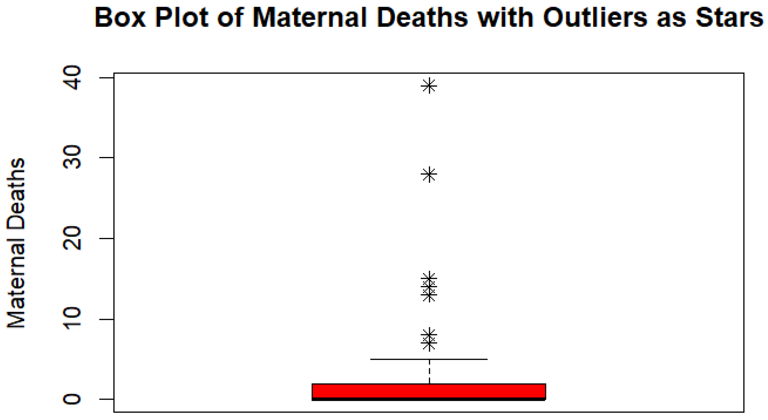
In examining the boxplot visualization of the maternal dataset in Figure 1, outliers are observed within the count variable, indicating instances where maternal deaths deviate significantly from the typical distribution. It is essential to recognize and comprehend these outliers, as they may affect the reliability and accuracy of inferences made from the dataset. To provide an accurate evaluation of what is impacting maternal mortality rates using robust count statistical modeling, it is vital to address the existence of outliers.

4.2.2. Assessment of Multicollinearity Test

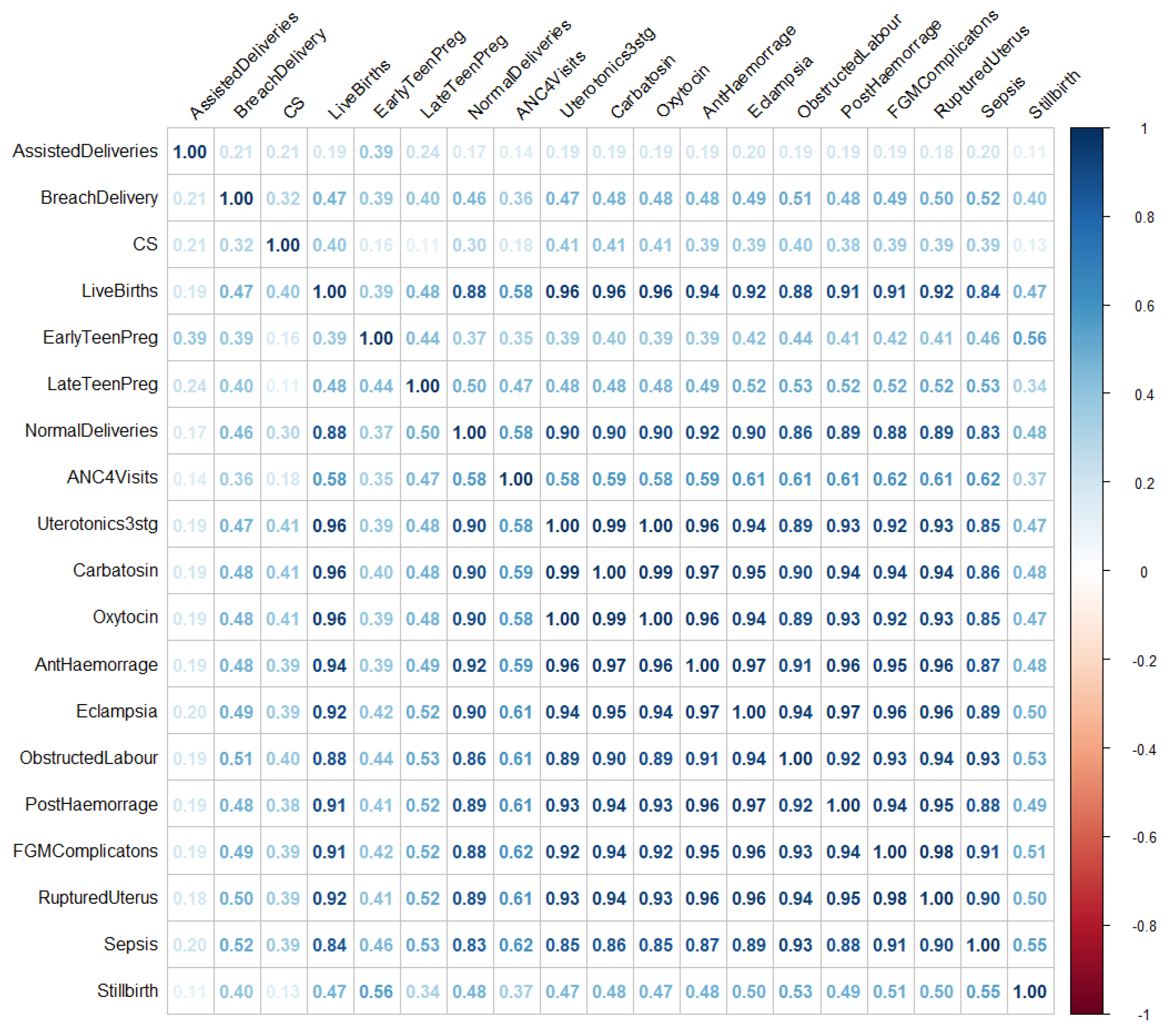
The analysis identified substantial correlations among several independent variables, indicating multicollinearity (see Figure 2). This issue arises when predictor variables are highly correlated, leading to redundancy and inflated standard errors in the regression coefficients. As a result, estimates become unstable, and theoretically important variables may appear statistically insignificant, obscuring their true relationships with the outcome.

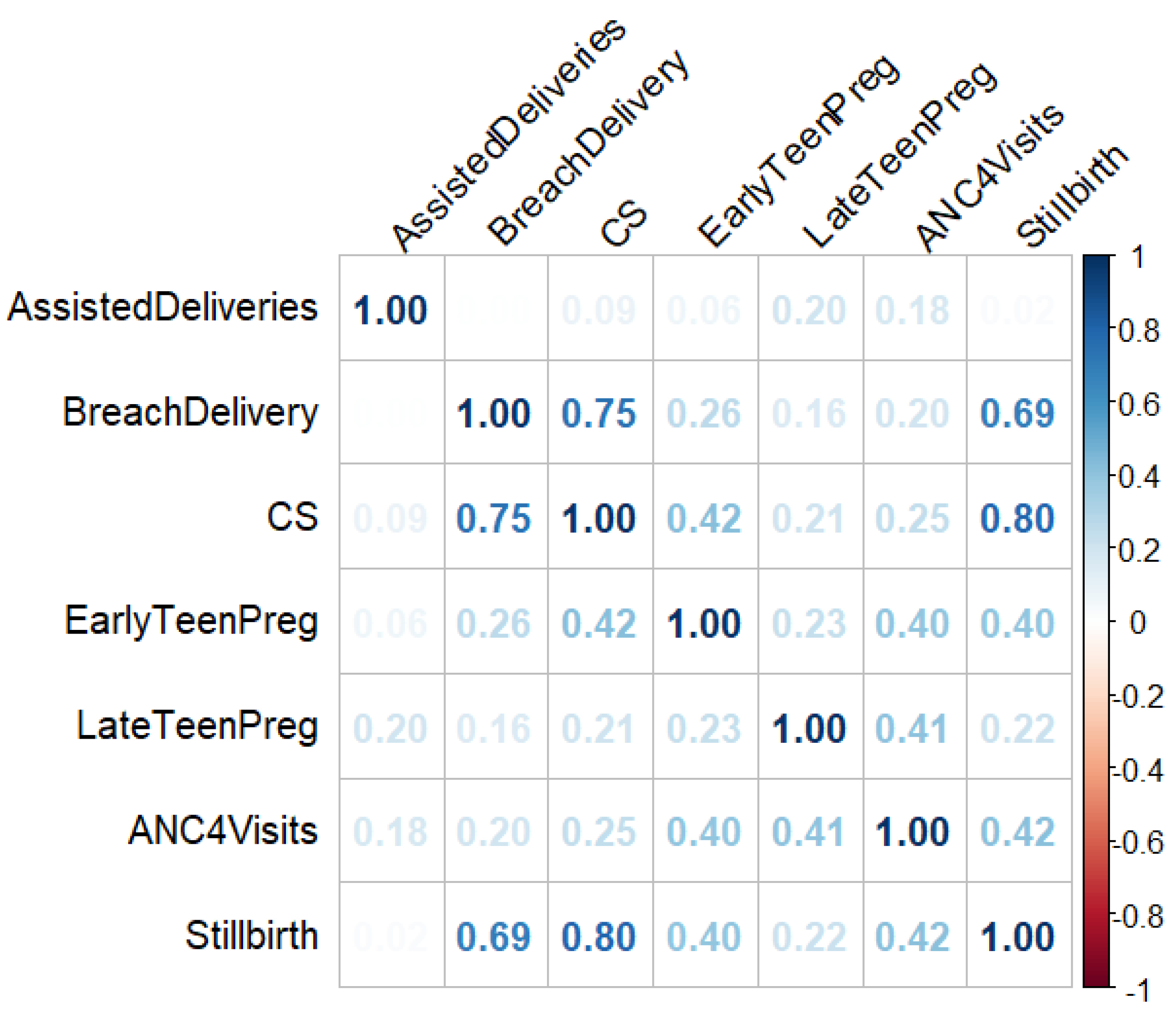
To mitigate multicollinearity between explanatory variables, a correlation-based feature selection technique was applied [21]. Variables exhibiting high linear correlation (|r| > 0.7) were examined, and from each highly correlated pair, one variable was excluded based on theoretical relevance, interpretability, and contribution to model performance. The updated correlation matrix shown in Figure 3 indicates a significant reduction in multicollinearity, confirming the effectiveness of the selection process. By removing highly correlated variables, the updated model, now free from the detrimental effects of high multicollinearity, provided more reliable and interpretable estimates. The reduction in multicollinearity is expected to improve the stability and reliability of the coefficient estimates. However, it is important to approach the interpretation of the results with caution. The relationships between the predictors and the outcome variable should be evaluated in the context of the selected variables.

4.2.3. Adjustment for Facility Size Through an Offset Term

To account for differences in the number of births handled by each healthcare facility, an offset term was included in all fitted count models. Facilities serving larger populations are naturally expected to record more maternal deaths, independent of underlying risk factors. Without this adjustment, model comparisons could be biased toward facilities with higher patient volumes. The offset term was defined as the natural logarithm of the total number of births recorded at each facility during the study period, denoted as $log\left({\mathrm{TotalBirths}}_i\right)$. Including this offset allows the models to estimate maternal mortality rates per birth rather than raw counts, ensuring fair comparisons across facilities of different sizes. Mathematically, the count component of the model becomes the following:

$$log\left({\mu }_i\right)={\beta }_0+{\beta }_1{x}_{i1}+\cdots +{\beta }_p{x}_{ip}+log\left({\mathrm{TotalBirths}}_i\right),$$

where ${\mu }_i$ is the expected number of maternal deaths at facility i, $x_{ij}$ are the predictor variables, and $log\left({\mathrm{TotalBirths}}_i\right)$ is the fixed offset term. For interpretability, the offset can also be scaled to express rates per 1000 births as $log({\mathrm{TotalBirths}}_i/1000)$. This adjustment ensures that model estimates reflect differences in maternal mortality risk, rather than differences in the volume of births handled by each facility.

4.3. Comparison of the Fitted Count Data Models

This is a comparison of all fitted models for maternal death counts using Akaike information criteria and Bayesian information criteria.

Table 3. Estimated AIC and BIC for the maternal mortality data.

Model	AIC	BIC
Poisson	249.039	265.880
NB	248.600	263.569
ZINB	231.808	268.242
HNB	240.032	276.466
RZIP	129.871	164.161
RZINB	131.804	168.237
RHP	136.419	170.709
RHNB	138.419	174.853

below provides the AIC and BIC values used to choose the model that best fits the data.

The comparison of the performance of the model in Table 3 reveals that the RZIP model provided the best fit to the data, outperforming all other models based on AIC and BIC. The NB model showed considerable improvement over the standard Poisson model, indicating its ability to handle overdispersion in the data more effectively. Among the robust models, the RZINB and RHP models showed competitive performance, especially the RZINB, but were still outperformed by the RZIP model. The RHNB model showed a slightly poorer fit compared to the RZIP, RHP, and RZINB models but performed better than the standard count (ZINB and HNB) and traditional (Poisson and NB) models. Looking at the ZINB, showed a better fit over the HNB and traditional models. These findings generally emphasize the suitability of the RZIP model for this dataset, demonstrating its ability to effectively address zero inflation and outliers at approximately 5%.

Figure 4 shows the observed histogram of maternal deaths overlaid with fitted probability curves from six different count regression models (Poisson, NB, RZIP, RZINB, RHP, and RHNB) that included covariates for assisted deliveries, breech delivery, early teen pregnancy, late teen pregnancy, attending at least four ANC visits (ANC4Visits), cesarean section (CS), and stillbirth. For each model, fitted probabilities were computed for individual observations using the estimated parameters and included covariates and then averaged across all observations to generate the marginal predicted distribution. This approach allows for a fair comparison with the empirical distribution of maternal deaths. The observed distribution exhibits significant excess zeros beyond what would be expected under standard count model assumptions, as also shown in Table 2. This zero inflation necessitates the evaluation of models explicitly designed to handle both structural and sampling zeros. The standard Poisson model performs poorly due to its assumption of equidispersion (equal mean and variance), leading it to severely underestimate the frequency of zero outcomes. Although the NB model partially addresses this by accommodating overdispersion, it still lacks a mechanism to model excess structural zeros. In contrast, the robust hurdle models (RHNB and RHP) and robust zero-inflated models (RZINB and RZIP) offer superior fits by explicitly modeling the dual processes that generate zero and positive counts separately. Among these, the RZIP model provides the best overall fit. Its two-part structure, separating the not-at-risk group (structural zeros) from the at-risk group (count component), enables it to accurately capture both the high frequency of zeros and the distribution of non-zero maternal deaths. These results are consistent with those in Table 3, where the RZIP achieved the lowest AIC and BIC scores.

4.4. Robust Count Regression Estimation Results

A significant frequency of zero counts and outliers was observed in the maternal mortality data. These observations deviate substantially from the expected patterns of standard count data distributions such as the Poisson and NB models. Such deviations suggest that the data may arise from two latent subpopulations, one that is not at risk of maternal mortality and thus always yields a count of zero, and another that is at risk and generates counts according to a standard count process (possibly zero or positive). In maternal mortality analysis, at-risk facilities are those that conduct deliveries with potential complications, high-risk pregnancies, or limited access to advanced obstetric care, making maternal deaths possible. Not-at-risk facilities are structurally unlikely to report maternal deaths because they either do not offer delivery services, handle only low-risk births, transfer complicated cases, or operate solely as antenatal/postnatal clinics. Furthermore, the presence of outliers in the data requires the use of robust estimation techniques, which the standard count models cannot account for. Given these challenges, an RZIP model is identified as the most appropriate for this analysis, as shown in Figure 4 and supported by model comparison results in Table 3. In the following

Table 4. Model estimation of coefficients using robust zero-inflated models.

Parameter	RZIP (Count Model)		RZIP (Zero Model)
	Estimate (SE)	p-Value	Estimate (SE)	p-Value
Intercept	1.6043 (0.1131)	-	11.0051 (6.8591)	-
BreachDelivery	0.2813 (0.0293)	$0.0251$	−0.5700 (0.1646)	0.5500
AssistedDeliveries	−0.5130 (0.0417)	$0.8435$	0.1189 (0.2146)	$0.8560$
EarlyTeenPreg	0.1621 (0.0304)	$0.0185$	0.6093 (0.4903)	0.2140
LateTeenPreg	−0.0086 (0.0325)	0.7900	0.0704 (0.2177)	0.0306
ANC4Visits	−0.2161 (0.0424)	$0.0319$	2.2527 (0.9386)	0.0164
CS	−0.0546 (0.0273)	$0.6580$	0.6830 (2.0994)	0.0015
Stillbirth	0.2835 (0.0305)	$0.0140$	−2.9196 (9.6433)	0.9862

, the study displays parameter estimates and the robust standard error of the best-performing model, which is RZIP.

Table 4 displays the estimated coefficients of the RZIP model for two parts, namely the count model and the zero model. The zero model explains the excess zeros in the data, while the count model concentrates on the count (frequency) of the event, which is maternal mortality in our case. Each component describes a distinct feature of the data. In the count component, the RZIP model estimates the expected number of maternal deaths per 1000 births among the at-risk group. The estimated intercept is $0.2002(SE=0.2722)$, which corresponds to an expected count of 0.4245 maternal deaths when all predictors are at their baseline levels. This significantly lower baseline suggests that, in the absence of specific risk factors, maternal mortality remains below the mean of the sample. Among predictors, BreachDelivery has a statistically significant positive effect on maternal mortality among the at-risk group, with an estimated coefficient of 0.2813 (p = 0.0251), corresponding to a $32.48\%$ increase in the expected number of maternal deaths per 1000 births $(e^{0.2813}-1=0.3248)$, reinforcing its role as a critical risk factor. Conversely, AssistedDeliveries do not exhibit a meaningful impact, with an estimated effect of $-0.5130(SE=0.0417,$ p = 0.8435), in the at-risk group $(e^{-0.5130}-1=-0.4013)$, corresponding to a 40.13% decrease in the expected number of maternal deaths per 1000 births of an individual being in an at-risk group in maternal mortality, suggesting a limited influence on maternal mortality among individuals at risk. EarlyTeenPreg, however, shows a notable positive association in the at-risk group, with an estimated coefficient of $0.1621(SE=0.0304$, p = 0.0185), indicating a $\mathit{17}.\mathit{59}\%$ increase in the expected count of maternal deaths per 1000 births among individuals at risk $(e^{0.1621}-1=0.1759)$. The statistical significance of this effect suggests that early teenage pregnancy is an important predictor of maternal mortality within the at-risk group.

LateTeenPreg, on the other hand, has an estimated effect of $-0.0863(SE=0.0325$, p = 0.7900), in the at-risk group corresponding to a 8.26% decrease in the expected count of maternal deaths per 1000 births $(e^{-0.0863}-1=-0.0826)$. However, this effect is not statistically significant ($p>$ 0.05), suggesting that late teenage pregnancy may not be a strong predictor of maternal mortality among individuals at risk. ANC4Visits and CS are both negatively associated with maternal mortality among individuals at risk, based on the count component of the model. ANC4Visits shows a statistically significant effect, with a $19.46\%$ decrease in the expected count of maternal deaths per 1000 births $(e^{-0.2161}-1=-0.1946)$, Although CS is associated with a $5.31\%$ decrease in the expected number of maternal death per 1000 births $(e^{-0.0546}-1=-0.0531)$, this effect is not statistically significant, indicating limited evidence of its independent contribution within the at-risk population. In contrast, StillBirth shows a positive significant effect, with a $32.77\%$ increase in the expected count of maternal deaths per 1000 births $(e^{0.2835}-1=0.3277)$. This finding strongly strengthens the critical role of stillbirth as a key risk factor for maternal mortality among at-risk individuals and emphasizes the need for targeted interventions addressing this factor to reduce maternal deaths.

The zero inflation component models the log-odds of belonging to the not-at-risk group, those for whom maternal mortality cannot occur (i.e., they always yield a zero count). Among predictors, BreachDelivery has an estimated effect of $-0.5700(SE=0.1646$, p = 0.5500), implying a $43.45\%$ decreased odds of an individual being in the not-at-risk group $(e^{-1.8413}-1=-0.8413)$, suggesting a limited influence on maternal mortality among individuals that are not-at-risk group. Similarly, AssistedDeliveries has an estimated effect of $0.1189(SE=0.2146$, p = 0.8560), suggesting a limited influence on maternal mortality among individuals who are not-at-risk group. EarlyTeenPreg has an estimated effect of $0.6093(SE=4903$, p = 0.2140), suggesting that for each unit increase in early teenage pregnancies, the odds of belonging to the not-at-risk group $(e^{0.6093}-1=0.8391)$, but there is limited influence on maternal mortality among individuals not-at-risk $(p>$ 0.05) indicating no strong evidence. In contrast, LateTeenPreg demonstrates a significant association in the zero-inflation component, with an estimated coefficient of $0.0704(SE=0.2177$, p = 0.0306), indicating a $7.29\%$ increase in the odds of being in the not-at-risk group $(e^{0.0704}-1=0.0729)$. This implies that regions with higher late teenage pregnancy rates may be more likely to fall into a subgroup structurally unlikely to report maternal deaths, possibly reflecting reporting differences or underlying protective mechanisms.

ANC4Visits has a statistically significant positive effect, with an estimated coefficient of $2.2527(SE=0.9386$, p = 0.0164), suggesting that for each unit increase in ANC4Visits pregnancies, the odds of belonging to the not-at-risk group $(e^{2.2527}-1=8.5133)$. This result suggests that higher ANC4Visits is associated with a substantially greater probability of avoiding maternal death, indicating that antenatal care may play a protective role in identifying or preventing risk before it manifests. The significance of this effect strengthens the importance of ANC4Visits in reducing the likelihood of being at risk for maternal mortality. CS has an estimated coefficient of $0.6830(SE=2.0994$, $\mathit{p}=0.0015)$, corresponding to a $97.98\%$ increase in the odds of being in the not-at-risk group per unit increase $(e^{0.6830}-1=0.9798)$. This indicates that individuals with higher values of CS are significantly more likely to be in the not-at-risk group. Similarly, StillBirth has a negative estimated coefficient of $-2.9196(SE=9.6433$, $\mathit{p}=0.9862)$, suggesting a $94.60\%$ decrease in the odds of being in the not-at-risk group $(e^{-2.9196}-1=-0.9460)$. This estimate is also not statistically significant, and the large standard error reflects substantial uncertainty. Thus, there is no reliable evidence that StillBirth affects the likelihood of being in the not-at-risk group.

4.5. The RZIP Model Validation

The chi-squared test in

Table 5. Model validation results.

Statistic	Value
Chi-Square Statistic	220.203
Degrees of Freedom	214
p-value	0.371

was used to validate the model. The test statistic is 220.203 with 214 degrees of freedom. The p-value is 0.371, which is greater than the typical significance level of 0.05. This indicates that there is no evidence to reject the null hypothesis. Thus, the fit of the model to the data is adequate, and there is no significant lack of fit based on this test.

4.6. Overview of Application Results

Count part (Poisson mean with offset):

$$\begin{array}{cc}\hfill log\left({\mu }_i\right)& =1.6043+0.2813·{\mathrm{BreachDelivery}}_i-0.5130·{\mathrm{AssistedDeliveries}}_i\hfill \\ \hfill & +0.1621·{\mathrm{EarlyTeenPreg}}_i-0.0086·{\mathrm{LateTeenPreg}}_i-0.2161·{\mathrm{ANC}4\mathrm{Visits}}_i\hfill \\ \hfill & -0.0546·{\mathrm{CS}}_i+0.2835·{\mathrm{StillBirth}}_i+log\left({\mathrm{TotalBirths}}_i\right).\hfill \end{array}$$

(27)

Zero-inflation part (logistic model):

$$\begin{array}{cc}\hfill log\left({\displaystyle \frac{{\pi }_i}{1-{\pi }_i}}\right)& =11.0051-0.5700·{\mathrm{BreachDelivery}}_i+0.1189·{\mathrm{AssistedDeliveries}}_i\hfill \\ \hfill & +0.6093·{\mathrm{EarlyTeenPreg}}_i+0.0704·{\mathrm{LateTeenPreg}}_i+2.2527·{\mathrm{ANC}4\mathrm{Visits}}_i\hfill \\ \hfill & +0.6830·{\mathrm{CS}}_i-2.9196·{\mathrm{StillBirth}}_i.\hfill \end{array}$$

(28)

Probability model:

$$P(Y_i=y_i)=\left\{\begin{array}{cc}{\pi }_i+(1-{\pi }_i)·e^{-{\mu }_i},\hfill & y_i=0,\hfill \\ (1-{\pi }_i)·{\displaystyle \frac{{\mu }_i^{y_i}{e}^{-{\mu }_i}}{y_i!}},\hfill & y_i>0,\hfill \end{array}\right.$$

where ${\mu }_i$ and ${\pi }_i$ are defined above, and $log\left({\mathrm{TotalBirths}}_i\right)$ is included as an offset to adjust for differences in facility size.

5. Conclusions

This study examined the performance of various count regression models using both simulated and real maternal mortality data. The findings revealed that the RZIP model was the best performer when outlier (0–5%) and dispersion $(r=5)$ levels were low, making it the most suitable model for such conditions. This result was consistent across both real and simulated data. However, as outlier levels and dispersion increased, the RZINB and RHNB models provided a better fit and predictive accuracy. These models effectively handled datasets with extreme zero inflation and severe outliers, outperforming traditional Poisson and NB models. The AIC and BIC further confirmed the importance of robust zero-inflated models like RZIP in capturing data complexities. In general, RZIP is recommended for datasets with minimal outliers (≤5%), while RZINB and RHNB are better suited for highly dispersed data with severe outliers. These insights highlight the need for researchers to carefully assess model performance and assumptions when analyzing complex count data.

Analysis of the RZIP model showed some statistical significance of maternal mortality. Early teenage pregnancy was associated with a significantly increased risk of maternal death per 1000 births among the at-risk group. This emphasizes a lack of physiological and psychological readiness for childbirth from these young mothers, especially in low-resource settings where access to advanced obstetric care is limited. In alignment with Sustainable Development Goal (SDG) 3.2 [22], which aims to end preventable deaths of newborns and children under five, greater attention must be directed toward maternal health interventions that prioritize early screening and safe delivery methods, such as cesarean sections where medically appropriate. Moreover, the study confirmed that ANC4Visits were statistically significant in both components, positively associated with maternal death in the at-risk group, but also showed a significant increase in the odds of being in the not-at-risk group. In pursuit of the broader SDG 3 goals, health systems should implement tailored strategies that provide adolescent-friendly maternal health services, including education, early risk assessment, and access to skilled birth attendants. Future work should explore the development of a robust hybrid zero inflation model, which combines the strengths of zero-inflated and hurdle frameworks with robust estimation to better handle extreme zero inflation, overdispersion, and outliers. Addressing multicollinearity through techniques such as principal component analysis (PCA) or regularization can further enhance model accuracy.

References

1. Shahsavari, S.; Yaseri, M.; Hosseini, M.; Moghimbeigi, A. Robust Inference for Zero-Inflated Models with Outliers Applied to the Number of Involved Lymph Nodes in Patients with Breast Cancer. 2023. Available online: https://doi.org/10.21203/rs.3.rs-2692063/v1 (accessed on 29 May 2025).
2. Feng, C.X. A comparison of zero-inflated and hurdle models for modeling zero-inflated count data. J. Stat. Distrib. Appl. 2021, 8, 8. [Google Scholar] [CrossRef] [PubMed]
3. Lambert, D. Zero-inflated Poisson regression, with an application to defects in manufacturing. Technometrics 1992, 34, 1–14. [Google Scholar] [CrossRef]
4. Min, Y.; Agresti, A. Random effect models for repeated measures of zero-inflated count data. Stat. Model. 2005, 5, 1–19. [Google Scholar] [CrossRef]
5. Hall, D.B. Robust estimation for zero-inflated Poisson regression. Scand. J. Stat. 2010, 37, 237–252. [Google Scholar] [CrossRef]
6. Mullahy, J. Specification and testing of some modified count data models. J. Econom. 1986, 33, 341–365. [Google Scholar] [CrossRef]
7. Tüzen, F. A simulation study for count data models under varying degrees of outliers and zeros. Commun. Stat.—Simul. Comput. 2018, 49, 1078–1088. [Google Scholar] [CrossRef]
8. Tawiah, K.; Iddi, S.; Lotsi, A. On Zero-Inflated Hierarchical Poisson Models with Application to Maternal Mortality Data. Int. J. Math. Math. Sci. 2020, 2020, 1407320. [Google Scholar] [CrossRef]
9. Bassey, U.E.; Akinyemi, M.I.; Njoku, K.F. On Zero inflated models with applications to maternal healthcare utilization. Int. J. Math. Sci. Optim. Theory Appl. 2021, 7, 65–75. [Google Scholar] [CrossRef]
10. Abonazel, M.R.; El-sayed, S.M.; Saber, O.M. Performance of robust count regression estimators in the case of overdispersion, zero inflated, and outliers: Simulation study and application to German health data. Commun. Math. Biol. Neurosci. 2021, 2021, 55. [Google Scholar] [CrossRef]
11. Adehi, M.; Yakasai, A.; Dikko, H.; Asiribo, E.; Dahiru, T. Risk of maternal mortality using relative risk ratios obtained from poisson regression analysis. Int. J. Dev. Res. 2017, 7, 15405–15409. [Google Scholar]
12. Okello, S.; Otieno Omondi, E.; Odhiambo, C.O. Improving performance of hurdle models using rare-event weighted logistic regression: An application to maternal mortality data. R. Soc. Open Sci. 2023, 10, 221226. [Google Scholar] [CrossRef] [PubMed]
13. Chau, A.M.H.; Lo, E.C.M.; Wong, M.C.M.; Chu, C.H. Interpreting poisson regression models in dental caries studies. Caries Res. 2018, 52, 339–345. [Google Scholar] [CrossRef] [PubMed]
14. Dean, C.B.; Lundy, E.R. Overdispersion. Wiley StatsRef Stat. Ref. Online 2016, 1–9. [Google Scholar] [CrossRef]
15. Payne, E.H.; Hardin, J.W.; Egede, L.E.; Ramakrishnan, V.; Selassie, A.W.; Gebregziabher, M. Approaches for dealing with various sources of overdispersion in modeling count data: Scale adjustment versus modeling. Stat. Methods Med. Res. 2015, 26, 1802–1823. [Google Scholar] [CrossRef] [PubMed]
16. Shahsavari, S.; Moghimbeigi, A.; Kalhor, R.; Jafari, A.M.; Bagherpour-kalo, M.; Yaseri, M.; Hosseini, M. Zero-Inflated Count Regression Models in Solving Challenges Posed by Outlier-Prone Data; an Application to Length of Hospital Stay. Arch. Acad. Emerg. Med. 2024, 12, e13. [Google Scholar] [PubMed]
17. Huber, P.J. Robust estimation of a location parameter. In Breakthroughs in Statistics: Methodology and Distribution; Springer: Berlin/Heidelberg, Germany, 1992; pp. 492–518. [Google Scholar]
18. Cantoni, E.; Zedini, A. A robust version of the hurdlemodel. J. Stat. Plan. Inference 2011, 141, 1214–1223. [Google Scholar] [CrossRef]
19. Miranda, M.; Miranda, M.C.; Gomes, M.I. A robust hurdle poisson model in the estimation of the extremal index. In Recent Developments in Statistics and Data Science; Springer: Cham, Switzerland, 2022; pp. 15–28. [Google Scholar] [CrossRef]
20. Akaike, H. A new look at the statistical model identification. IEEE Trans. Autom. Control. 1974, 19, 716–723. [Google Scholar] [CrossRef]
21. Hall, M.A. Correlation-based feature selection of discrete and numeric class machine learning. In Proceedings of the Seventeenth International Conference on Machine Learning (ICML 2000), Stanford University, Stanford, CA, USA, 29 June–2 July 2000. [Google Scholar]
22. GBD 2019 Under-5 Mortality Collaborators. Global, regional, and national progress towards Sustainable Development Goal 3.2 for neonatal and child health: All-cause and cause-specific mortality findings from the Global Burden of Disease Study 2019. Lancet 2021, 398, 870–905. [Google Scholar]
Figure 1. Visualization of outliers.
Mca 30 00095 g001
Figure 2. Visualization indicating multicollinearity patterns.
Mca 30 00095 g002
Figure 3. Retained variables after multicollinearity screening.
Mca 30 00095 g003
Figure 4. Probability models for the number of maternal deaths.
Mca 30 00095 g004