Modeling of Nonlinear Systems: Method of Optimal Injections

Abstract

In this paper, a nonlinear system is interpreted as an operator $\mathcal{F}$ transforming random vectors. It is assumed that the operator is unknown and the random vectors are available. It is required to find a model of the system represented by a best constructive operator $\mathcal{F}$ approximation. While the theory of operator approximation with any given accuracy has been well elaborated, the theory of best constrained constructive operator approximation is not so well developed. Despite increasing demands from various applications, this subject is minimally tractable because of intrinsic difficulties with associated approximation techniques. This paper concerns the best constrained approximation of a nonlinear operator in probability spaces. The main conceptual novelty of the proposed approach is that, unlike the known techniques, it targets a constructive optimal determination of all $3p+2$ ingredients of the approximating operator where p is a nonnegative integer. The solution to the associated problem is represented by a combination of new best approximation techniques with a special iterative procedure. The proposed approximating model of the system has several degrees of freedom to minimize the associated error. In particular, one of the specific features of the developed approximating technique is special random vectors called injections. It is shown that the desired injection is determined from the solution of a special Fredholm integral equation of the second kind. Its solution is called the optimal injection. The determination of optimal injections in this way allows us to further minimize the associated error.

1. Introduction

1.1. Motivation

Over the last few decades, the problem of constructive approximation of nonlinear operators has been a topic of profound research. A number of fundamental papers have appeared, which have established significant advances in this research area. Some relevant references can be found, in particular, in [1,2,3,4,5,6,7,8,9,10,11,12,13,14].

The known related results mainly concern proving the existence and uniqueness of operators approximating a given map, and justifying the bounds of errors arising from the approximation methods. The assumptions are that preimages and images are deterministic and can be represented in an analytical form, that is, by equations. At the same time, in many applications, the sets of preimages and images are stochastic and cannot be described by equations. Nevertheless, it is possible to represent these sets in terms of their numerical characteristics, such as the expectation and covariance matrices. Typical examples include stochastic signal processing [15,16,17,18,19], statistics [20,21,22,23,24], engineering [25,26,27,28], and image processing [29,30]; in the latter case, a digitized image, presented by a matrix, is often interpreted as the sample of a stochastic signal.

While the theory of operator approximation with any given accuracy is well elaborated (see, e.g., [1,2,3,4,5,6,7,8,9,10,11,12,13,14]), the theory of best constrained constructive operator approximation is not particularly well developed, although this is an area of intensive recent research (see, e.g., [31,32,33,34,35,36]). Despite increasing demands from applications [17,18,19,21,22,23,25,26,27,28,30,31,32,33,34,36,37,38,39,40,41,42,43,44,45,46], this subject is minimally tractable because of intrinsic difficulties in best approximation techniques, especially when the approximating operator should have a specific structure implied by the underlying problem. Recent studies related to this topic can be found in [47,48,49,50,51,52,53,54,55]. In particular, in [47], an approach to modeling of nonlinear systems was proposed based on observed input-output data. The proposed method constructs an approximate model by decomposing the unknown function into multiple components, aiming to minimize the associated error. Special random vectors, called injections, are used to refine the approximation while specific transformations simplify the optimization process. The approach provides flexibility in adjusting parameters to improve accuracy.

We wish to extend the known results in this area to the case when the sets of preimages and images of map $\mathcal{F}$ are stochastic, and the approximating operator we search is constructive in the sense it can numerically be realized and, therefore, is applicable to problems in applications.

1.2. Short Description of the Method

Let $\Omega$ be a set of outcomes in the probability space $(\Omega ,\Sigma ,\mathit{\mu })$ for which $\Sigma$ is a $\mathit{\sigma }$–field of measurable subsets of $\Omega$ and $\mathit{\mu }:\Sigma \to [0,1]$ is an associated probability measure. Let $\mathbf{x}\in L^2(\Omega ,{\mathbb{R}}^m)$ and $\mathbf{y}\in L^2(\Omega ,{\mathbb{R}}^n)$ be random vectors, $\mathcal{F}:L^2(\Omega ,{\mathbb{R}}^n)\to L^2(\Omega ,{\mathbb{R}}^m)$ be a nonlinear map, and $\mathbf{x}=\mathcal{F}(\mathbf{y})$.

A nonlinear system is interpreted as the map $\mathcal{F}$ where $\mathbf{x}$ and $\mathbf{y}$ are random output and input signals, respectively. It is assumed that $\mathcal{F}$ is unknown, and $\mathbf{x}$ and $\mathbf{y}$ are available. We propose and justify a new method for the constructive $\mathcal{F}$ approximation such that first, an associated error is minimized and second, a structure of the approximating operator satisfies the special constraint related to the dimensionality reduction of vector $\mathbf{y}$. More specifically, we develop a new approach to the best constructive approximation of the map $\mathcal{F}$ in probability spaces subject to a specialized criterion associated with the dimensionality reduction of random preimages. The latter constraint follows from the requirements in applications such as those considered in [20,21,22,23,24,26,41,42]. In particular, in signal processing and system theory, a dimensionality reduction of random signals is used to optimize the cost of signal transmission. It is assumed that the only available information on $\mathcal{F}$ is given by certain covariance matrices formed from the preimages and images. This is a typical assumption used in applications such as those considered, e.g., in [15,16,17,18,19,20,21,22,23,37,38,44,45,46]. Here, we adopt that assumption. As mentioned, in particular, in [56,57,58,59,60,61], a priori knowledge of the covariances can come either from specific data models, or after sample estimation during a training phase.

The problem we consider (see (7) below) concerns finding the best approximating operator that depends on $2p+2$ unknown matrices $G_j$ and $H_j$, for $j=0,\dots ,p$ and p more unknown random vectors ${\mathbf{v}}_1,\dots ,{\mathbf{v}}_p$. We call ${\mathbf{v}}_1,\dots ,{\mathbf{v}}_p$ the injections. Here, p is a non-negative integer p. The injections ${\mathbf{v}}_1,\dots ,{\mathbf{v}}_p$ are aimed to further diminish the associated error. The difficulty is that $3p+2$ unknowns should be determined from a minimization of the single cost function given in (7).

The main difference between the approach in [47] and the method proposed in this paper is in their approach to modeling of nonlinear systems. The method in [47] constructs the model ${\mathcal{T}}_p$ as a sum of $p+1$ specific components, and the original optimization problem is decomposed into $p+1$ simpler sub-problems. The method empirically determines the special random vectors, called injections, to reduce the associated error. In contrast, the method proposed here solves the problem of a best constrained approximation of a nonlinear operator in probability spaces. It introduces the concept of an optimal injection, which is determined by solving a Fredholm integral equation of the second kind. While the method in [47] focuses on a structured numerical implementation, the proposed method provides a more general theoretical framework that optimally determines all $3p+2$ parameters through a combination of best approximation techniques and an iterative procedure.

The solution is represented in Section 3 and Section 4, and is based on the following observation. Methods for best approximation are aimed at obtaining the best solution within a certain class; the accuracy of the solution is limited by the extent to which the class is satisfactory. By contrast, iterative methods are normally convergent, but the convergence can be quite slow. Moreover, in practice, only a finite number of iteration loops can be carried out, and therefore, the final approximate solution is often unsatisfactorily inaccurate. A natural idea is to combine the methods for best approximation and iterative techniques to exploit their advantageous features.

In Section 3 and Section 4, we present an approach which realizes this. First, a special iterative procedure is proposed which aims to improve the accuracy of approximation with each consequent iteration loop. Secondly, the best approximation problem is solved providing the smallest associated error within the chosen class of approximants for each iteration loop. In Section 4, we show that the combination of these techniques allows us to build a computationally efficient and flexible method. In particular, we prove that the error in approximating $\mathcal{F}$ by the proposed method decreases with an increase in the number of iterations. An application is made to the optimal filtering of stochastic signals.

1.3. Novelty and Advantages

The novelty of the proposed method is in its approach to the best constructive approximation of nonlinear operators in probability spaces. Unlike methods that primarily focus on the existence and uniqueness of approximating operators, the proposed method aims to achieve an optimal constructive approximation by targeting a specific structure for the approximating operator, which is constrained by dimensionality reduction of random preimages. The focus on dimensionality reduction and the optimization of random vectors, known as injections, distinguishes the proposed method from existing approaches.

The advantages of the proposed method are twofold. First, it allows us to determine optimal injections which are derived from solving a Fredholm integral equation of the second kind, thereby providing a more robust and theoretically sound approach to approximating nonlinear systems. Second, the method combines best approximation techniques with a special iterative procedure, ensuring that the accuracy of the approximation improves with each iteration. This combination not only enhances the computational efficiency of the model but also provides a flexible framework that can be adapted to various applications, particularly those associated with signal processing and system theory, where dimensionality reduction plays a crucial role in optimizing signal transmission costs. By approximating $\mathcal{F}$ using the best constrained constructive operator approximation, one can design efficient algorithms for signal reconstruction or denoising. In system identification, this approach can be used to model and estimate dynamic systems with stochastic inputs, enabling more accurate predictions and adaptive control strategies.

2. The Proposed Approach

2.1. Some Special Notation

Let us write $\mathbf{x}={[{\mathbf{x}}_{(1)},\dots ,{\mathbf{x}}_{(m)}]}^T$ and $\mathbf{y}={[{\mathbf{y}}_{(1)},\dots ,{\mathbf{y}}_{(n)}]}^T$ where ${\mathbf{x}}_{(i)},{\mathbf{y}}_{(j)}\in L^2(\Omega ,\mathbb{R})$, for $i=1,\dots ,m$ and $j=1,\dots ,n$, and $\mathbf{x}(\omega )\in {\mathbb{R}}^m$ and $\mathbf{y}(\omega )\in {\mathbb{R}}^n$ for all $\omega \in \Omega$. Each matrix $A\in {\mathbb{R}}^{m\times n}$ defines a bounded linear transformation $\mathcal{A}:L^2(\Omega ,{\mathbb{R}}^n)\to L^2(\Omega ,{\mathbb{R}}^m)$. It is customary to write A rather then $\mathcal{A}$ since $[\mathcal{A}(\mathbf{x})](\omega )=A[\mathbf{x}(\omega )]$, for each $\omega \in \Omega$. Let us also write

$$\begin{array}{c}\hfill {\parallel \mathbf{x}\parallel }_{\Omega }^2={\int }_{\Omega }{\displaystyle \sum _{j=1}^m}{\left[{\mathbf{x}}_j(\omega )\right]}^{2}d\mathit{\mu }(\omega )<\infty .\end{array}$$

(1)

The covariance matrix formed from $\mathbf{x}$ and $\mathbf{y}$ is denoted by $E_{xy}$ such that

$$\begin{array}{c}\hfill E_{xy}={\int }_{\Omega }\mathbf{x}(\omega ){\left[\mathbf{y}(\omega )\right]}^{T}d\mathit{\mu }(\omega )={\left\{{\int }_{\Omega }{\mathbf{x}}_{(i)}(\omega ){\mathbf{y}}_{(j)}(\omega )d\mathit{\mu }(\omega )\right\}}_{i,j=1}^{m,n}.\end{array}$$

(2)

The Moore–Penrose pseudo-inverse [62] of matrix M is denoted by $M^{†}$.

2.2. Generic Structure of Approximating Operator

Let ${\mathbf{v}}_1,\dots ,{\mathbf{v}}_p$ be random vectors such that ${\mathbf{v}}_j\in L^2(\Omega ,{\mathbb{R}}^{q_j})$, for $j=1,\dots ,p$. We write $\mathbf{y}={\mathbf{v}}_0$ and $q_0=n$. As mentioned before, we call ${\mathbf{v}}_1,\dots ,{\mathbf{v}}_p$ the injections. This is because ${\mathbf{v}}_1,\dots ,{\mathbf{v}}_p$ contribute to the decrease of the associated error, as shown in Section 4.4 below. The choice of ${\mathbf{v}}_1,\dots ,{\mathbf{v}}_p$ is considered in Section 4.2, where each ${\mathbf{v}}_j$, for $j=1,\dots ,p$ is defined by a nonlinear transformation ${\phi }_j$ of $\mathbf{y}$, i.e., ${\mathbf{v}}_j={\phi }_j(\mathbf{y})$. To facilitate the numerical implementation of the approximating technique introduced below, each vector ${\mathbf{v}}_j$, for $j=1,\dots ,p$, is transformed to vector ${\mathbf{z}}_j\in L^2(\Omega ,{\mathbb{R}}^{q_j})$ by transformation $Q_j$ so that

$$\begin{array}{c}\hfill {\mathbf{z}}_j=Q_j({\mathbf{v}}_j,Z_{j-1}),\end{array}$$

(3)

where $Z_{j-1}=\{{\mathbf{z}}_0,\dots ,{\mathbf{z}}_{j-1}\}$. The choice of $Q_j$ is considered in Section 3.1.

Further, for $i=0,1,\dots ,p$, let $G_i\in {\mathbb{R}}^{m\times r_i},$ $H_i\in {\mathbb{R}}^{r_i\times q_i}$ where $r_i$ is given, $0<r_i<r$, and

$$\begin{array}{c}\hfill r=r_0+\dots +r_p.\end{array}$$

(4)

Here, r is a positive integer such that $r\le min\{m,n\}$.

It is convenient to set $Q_0=I$ and ${\mathbf{z}}_0={\mathbf{v}}_0=\mathbf{y}$. To approximate $\mathcal{F}$ for a given reduction ratio

$$\begin{array}{c}\hfill {\displaystyle c=r/min\{m,n\},}\end{array}$$

(5)

we consider operator ${\mathcal{T}}_p:L^2(\Omega ,{\mathbb{R}}^{q_0})\times \dots \times L^2(\Omega ,{\mathbb{R}}^{q_p})\to L^2(\Omega ,{\mathbb{R}}^m)$ represented by

$$\begin{array}{c}\hfill {\mathcal{T}}_p({\mathbf{v}}_0,\dots {\mathbf{v}}_p)=G_0{H}_0{\mathbf{z}}_0+\dots +G_p{H}_p{\mathbf{z}}_p,\end{array}$$

(6)

where $G_j:L^2(\Omega ,{\mathbb{R}}^{r_j})\to L^2(\Omega ,{\mathbb{R}}^m)$ and $H_j:L^2(\Omega ,{\mathbb{R}}^{q_j})\to L^2(\Omega ,{\mathbb{R}}^{r_j})$, for $j=0,1,\dots ,p$, are linear operators (i.e., $G_j$ and $H_j$ are represented by $m\times r_j$ and $r_j\times q_j$ matrices, respectively. Recall that we use the same symbol to define a matrix and the associated linear operator).

Importantly, operators $H_0,\dots ,H_p$ imply the dimensionality reduction of vector $\mathbf{y}$. This is because $H_i{\mathbf{z}}_i\in L^2(\Omega ,{\mathbb{R}}^{r_i})$ where $0<r_i<r\le min\{m,n\}$, for $i=0,\dots ,p$.

We call p the degree of ${\mathcal{T}}_p$. It is shown below that ${\mathcal{T}}_p$ approximates an operator of interest $\mathcal{F}:L^2(\Omega ,{\mathbb{R}}^n)\to L^2(\Omega ,{\mathbb{R}}^m)$, with the accuracy represented by theorems in Section 3.3, Section 3.4, and Section 4.4.

2.3. Statement of the Problem

Let $\mathcal{F}:L^2(\Omega ,{\mathbb{R}}^n)\to L^2(\Omega ,{\mathbb{R}}^m)$ be a continuous operator. We consider the problem as follows: Given $\mathbf{x},\mathbf{y}$ and $r_0,\dots ,r_p$, find matrices $G_0,H_0,\dots ,G_p,H_p$ and vectors ${\mathbf{v}}_1,$ $\dots ,{\mathbf{v}}_p$ that solve

$$\begin{array}{c}\hfill {\displaystyle \underset{{\mathbf{v}}_1,\dots ,{\mathbf{v}}_p}{min}}{\displaystyle \underset{\begin{array}{c}{G}_0,H_0,\dots ,G_p,H_p\end{array}}{min}}{∥\mathcal{F}(\mathbf{y})-{\displaystyle \sum _{j=0}^p}{G}_j{H}_j{\mathbf{z}}_j∥}_{\Omega }^2\end{array}$$

(7)

subject to

$$\begin{array}{c}\hfill G_j\in {\mathbb{R}}^{m\times r_j}\mathrm{and}{H}_j\in {\mathbb{R}}^{r_j\times q_j},\end{array}$$

(8)

and

$$\begin{array}{c}\hfill E_{z_i{z}_j}=\mathbb{O},\mathrm{for}i\ne j,\end{array}$$

(9)

where $i,j=0,\dots ,p$ and $\mathbb{O}$ denotes the zero matrix (and the zero vector).

It will be shown in Section 3 below that the solution of problem (7)–(9) is determined under a special condition imposed on vectors ${\mathbf{v}}_1,\dots ,{\mathbf{v}}_p$.

2.4. Related Work

2.4.1. Low-Rank Approximations

For $p=0$ and the assumption that matrix $E_{xy}$ is invertible, the particular case of the problem in (7)–(9),

$$\begin{array}{c}\hfill {\displaystyle \underset{G_0,H_0}{min}}{∥\mathbf{x}-G_0{H}_0\mathbf{y}∥}_{\Omega }^2,\end{array}$$

(10)

has been solved, in particular, in [20,21,63,64,65]. Under the assumption $E_{xy}$ is singular, it has been solved in [24,66,67,68,69]. Note it is a quite simplified case of problem in (7)–(9).

For $p=1$, $G:L^2(\Omega ,{\mathbb{R}}^{r_0})\to L^2(\Omega ,{\mathbb{R}}^m)$, $H_j:L^2(\Omega ,{\mathbb{R}}^n)\to L^2(\Omega ,{\mathbb{R}}^{r_0})$ where $j=0,1$, a particular case of the problem in (7)–(9),

$$\begin{array}{c}\hfill {\displaystyle \underset{G,H_0,H_1}{min}}{\parallel \mathbf{x}-G(H_0\mathbf{y}+H_1{\mathbf{v}}_1)\parallel }_{\Omega }^2,\end{array}$$

(11)

was solved in [20]. The choice of ${\mathbf{v}}_1$ considered in [20] is not optimal.

2.4.2. Tensor Methods

In [70,71,72], the problem in (10) is generalized and studied in terms of tensors. Together with methods formulated in terms of matrices and mentioned in Section 1 and Section 2.4.1, the tensor methods represent an important research subject both in the theoretical and applied sense. In this paper, the problems in (10) and (11) are generalized in a different way, which was described in Section 2.2 and Section 2.3, and will be justified in Section 3 and Section 4.4 below.

2.4.3. System Identification and Modeling

The problem we consider can also be represented as a black-box problem [73,74] where $\mathbf{y}$ and $\mathbf{x}$ are an available random input and output, respectively, and $\mathcal{F}$ is an unknown system. Then, the approximating operator ${\mathcal{T}}_p$ identifies a model of the system. Its particular features are detailed in Section 4.

2.5. Contribution

2.5.1. Challenges of High-Dimensionality

The proposed approach achieves the dimensionality reduction of preimages in the following way. In (6), let us write ${\mathcal{T}}_p({\mathbf{v}}_0,\dots {\mathbf{v}}_p)$ as

$${\displaystyle {\mathcal{T}}_p({\mathbf{v}}_0,\dots {\mathbf{v}}_p)=[G_0,\dots ,G_p]\left[\begin{array}{c}{H}_0{\mathbf{z}}_0\\ ⋮\\ H_p{\mathbf{z}}_p\end{array}\right]=GH\mathbf{z},}$$

where $G=[G_0,\dots ,G_p]$, $H=\mathrm{diag}[H_0,\dots ,H_p]$, $\mathbf{z}={[{\mathbf{z}}_0^T,\dots ,{\mathbf{z}}_p^T]}^T$. Here, H is the block-diagonal matrix with $H_0,\dots ,H_p$ on the main diagonal and the dimensionality of vector $\mathbf{u}=H\mathbf{z}$ is r, which is defined by (4). Therefore, H realizes the dimensionality reduction in vector $\mathbf{y}$ with the reduction ratio defined by (5). Unlike the known techniques [20,21,22,23,24,26,41,42] for dimensionality reduction, the proposed approach achieves this by using $p+1$ terms, $H_0,\dots ,H_p$. This allows us to increase the accuracy associated with optimal determination of approximating operator ${\mathcal{T}}_p$. More details can be found in Section 2.5.3 and Section 4.

2.5.2. Challenges of Accuracy

It is shown in Theorems 3, 4, and 5 below that, for the same reduction ratio, accuracy associated with the approximating operator ${\mathcal{T}}_p$ improves if the degree p or dimensions of injections ${\mathbf{v}}_1,\dots ,{\mathbf{v}}_p$ increase. For the case of the optimal determination of injections ${\mathbf{v}}_1,\dots ,{\mathbf{v}}_p$, the associated error is further improved. This is established in Theorems 10 and 11 in Section 4.4.

2.5.3. Novelties and Relation to Existing Concepts

Commonly, an approximating operator is represented by ${\sum }_{j=0}^p{P}_j{\mathbf{v}}_j$ where ${\mathbf{v}}_0,\dots ,{\mathbf{v}}_p$ are known basis functions and $P_0,\dots ,P_j$ are scalars or matrices which should be determined from (desirably) an error minimization.

The main conceptual novelty of the proposed approach is that, unlike the known techniques, it targets a constructive optimal determination of all $3p+2$ ingredients of the approximating operator in (6). They are ${\mathbf{v}}_1,\dots ,{\mathbf{v}}_p,H_0,G_0,\dots ,$ $H_p,G_p$. The solution of the associated problem (7)–(9) is provided in Section 3.1, Section 3.2, Section 4.1, and Section 4.2, and is represented by a combination of a new best approximation technique with a special iterative procedure.

A basic idea of the solution is to reduce the original problem (7)–(9) with $3p+2$ unknowns to $p+1$ simpler problems in (25) and (63) so that each of them, for $j=1,\dots ,p$, contains only three unknowns, ${\mathbf{v}}_j,H_j$, and $G_j$. For $j=0$, there are only two unknowns, $H_0$ and $G_0$. This is achieved due to exploiting operators $Q_0,\dots ,Q_p$ determined in Theorem 1.

The iteration procedure represented in Section 4.1 is based on the idea of the maximum block improvement method [75] which is an efficient technique for solving the spherically constrained homogeneous polynomial optimization problems. The associated novelties are in the techniques for the determination of matrices $H_0,G_0,\dots ,$ $H_p,G_p$ given in Section 3.2, injections ${\mathbf{v}}_1,\dots ,{\mathbf{v}}_p$ represented in Section 4.2, and for the error analysis given in Section 3.3 and Section 4.4. In particular, it is shown in Theorem 8 in Section 4.2 that the desired vector ${\mathbf{v}}_j$ is determined from the solution of a special Fredholm integral equation of the second kind (71). Its solution is called the optimal injection.

Further, unlike the known techniques, the proposed approximating operator ${\mathcal{T}}_p$ has several degrees of freedom to minimize the associated error. They are:

• ‘degree’ p of ${\mathcal{T}}_p$,
• matrices $G_0,H_0,\dots ,$ $G_p,H_p$,
• optimal injections ${\mathbf{v}}_1,\dots ,{\mathbf{v}}_p$,
• values of $r_0,\dots ,r_p$ in (4), and
• dimensions $q_1,\dots ,q_p$ of injections ${\mathbf{v}}_1,\dots ,{\mathbf{v}}_p$.

It is shown in Section 3.3 and Section 4.4 below that both the optimal choice of $G_0,H_0,\dots ,$ $G_p,H_p$ and injections ${\mathbf{v}}_1,\dots ,{\mathbf{v}}_p$, and the increase in $r_0,\dots ,r_p$ and $q_1,\dots ,q_p$ lead to the decrease in the error associated with approximating operator ${\mathcal{T}}_p$. Injections ${\mathbf{v}}_1,\dots ,{\mathbf{v}}_p$ represent a new special feature of the proposed technique.

In terms of multilayer networks, the novelties are as follows. First, the associated network consists of four hidden layers, i.e., more than in the known networks. Second, it exploits the interaction between the hidden layers (see Figure 1 where a particular case of ${\mathcal{T}}_p({\mathbf{v}}_0,\dots ,{\mathbf{v}}_p)$ for $p=3$ is illustrated). These particular features imply the improvement in the associated accuracy (see Section 3.3 and Section 4.4). In Figure 1, $\tilde{\mathbf{x}}$ denotes the approximation of $\mathbf{x}=\mathcal{F}(\mathbf{y})$ determined by the proposed technique, i.e., $\tilde{\mathbf{x}}={\mathcal{T}}_p({\mathbf{v}}_0,\dots ,{\mathbf{v}}_p)$. Details are provided in Section 4.

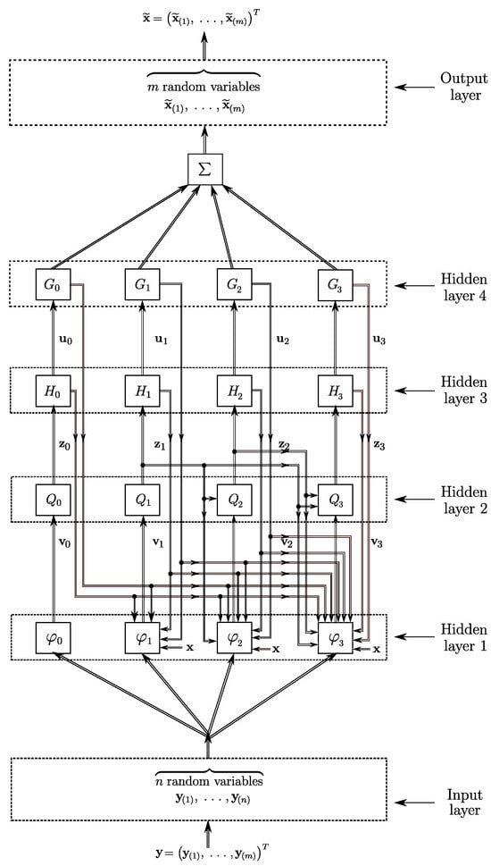
Figure 1. Diagrammatical representation of the proposed technique.

In terms of system identification, side by side with the black-box problem as in [73,74], the problem in (7)–(9) can be interpreted as a quite wide generalization of the blind system identification problem considered, in particular, in [17,76,77,78]. This is because vectors ${\mathbf{v}}_1,\dots ,{\mathbf{v}}_p$ are assumed to be unknown. Unlike the existing work on blind system identification, the problem in (7)–(9) is stated in terms of random vectors. Other novelties associated with system identification are similar to those considered above, i.e., the proposed model ${\mathcal{T}}_p({\mathbf{v}}_0,\dots ,{\mathbf{v}}_p)$ of the system contains $2p+1$ unknowns, the method of their determination is different from the existing techniques, and the associated accuracy is improved by a variation in more degrees of freedom.

3. Preliminary Results

Here, we consider the determination of vectors ${\mathbf{z}}_1,\dots ,$ ${\mathbf{z}}_p$ (in Definition 1 that follows, they are called pairwise uncorrelated vectors) and the solution of a particular case of the problem in (7), (8), (9) where the minimization with respect to ${\mathbf{v}}_1,\dots ,$ ${\mathbf{v}}_p$ is not included. These preliminary results will be used in Section 4, where the solution to the original problem represented by (7), (8), (9) is provided.

Definition 1.

Random vectors ${\mathbf{z}}_0,\dots ,{\mathbf{z}}_p$ are called pairwise uncorrelated if the condition in (9) holds for any pair of vectors ${\mathbf{z}}_i$ and ${\mathbf{z}}_j$, for $i\ne j$, where $i,j=0,\dots ,p$. Two vectors ${\mathbf{z}}_i$ and ${\mathbf{z}}_j$ belonging to the set of the pairwise uncorrelated vectors are called uncorrelated.

For $j=0,\dots ,p$, let $\mathcal{N}(M^{(j)})$ be a null space of matrix $M^{(j)}\in {\mathbb{R}}^{q_j\times q_j}$.

Definition 2.

Random vectors ${\mathbf{v}}_0,\dots ,{\mathbf{v}}_p$ are called linearly independent in the generalized sense if, for every collection of matrices $M^{(0)},\dots ,M^{(p)}$,

$$M^{(0)}{\mathbf{v}}_0(\omega )+\dots +M^{(p)}{\mathbf{v}}_p(\omega )=\mathbb{O},$$

 for almost all $\omega \in \Omega$, implies that ${\mathbf{v}}_j(\omega )\in \mathcal{N}(M^{(j)})$, for each $j=0,\dots ,p$, and almost all $\omega \in \Omega$.

Definition 3.

Random vector ${\mathbf{v}}_j$, for $j=0,\dots ,p,$ is called the well-defined injection if

$$\begin{array}{c}\hfill {\Gamma }_{z_j}=E_{x{z}_j}{E}_{z_j{z}_j}^{†}{E}_{z_{j}x}\ne \mathbb{O},\end{array}$$

(12)

where ${\mathbf{z}}_{\mathbf{j}}$ is defined by (3). Otherwise, injection ${\mathbf{v}}_j$ is called ill-defined.

An explanation for introducing Definition 3 is provided by Remark 1 at the end of Section 3.2 below.

3.1. Determination of Pairwise Uncorrelated Vectors

Theorem 1.

Let random vectors ${\mathbf{v}}_0,\dots ,{\mathbf{v}}_p$ be linearly independent in the generalized sense. Then they are transformed to the pairwise uncorrelated vectors ${\mathbf{z}}_0,\dots ,{\mathbf{z}}_p$ by transformations $Q_0,\dots ,Q_p$ as follows:

$$\begin{array}{ccc}\hfill & & {\mathbf{z}}_0=Q_0({\mathbf{v}}_0)={\mathbf{v}}_0\mathit{and}\mathit{,}\mathit{for}j=1,\dots ,p,\hfill \end{array}$$

(13)

$$\begin{array}{ccc}& & {\mathbf{z}}_j=Q_j({\mathbf{v}}_j,Z_{j-1})={\mathbf{v}}_j-{\displaystyle \sum _{k=0}^{j-1}}{E}_{v_j{z}_k}{E}_{z_k{z}_k}^{†}{\mathbf{z}}_k.\hfill \end{array}$$

(14)

Proof. 

Suppose that the condition in (9) holds for ${\mathbf{z}}_0,$ $\dots ,{\mathbf{z}}_{i-1}$. Then, for $\mathit{\ell }=0,\dots ,i-1$,

$$\begin{array}{ccc}\hfill E_{z_i{z}_{\mathit{\ell }}}& =& E[({\mathbf{v}}_i-{\displaystyle \sum _{l=0}^{i-1}}{E}_{v_i{z}_l}{E}_{z_l{z}_l}^{†}{\mathbf{z}}_l){\mathbf{z}}_{\mathit{\ell }}^T]\hfill \\ & =& E_{v_i{z}_{\mathit{\ell }}}-{\displaystyle \sum _{l=0}^{i-1}}{E}_{v_i{z}_l}{E}_{z_l{z}_l}^{†}{E}_{z_l{z}_{\mathit{\ell }}}\hfill \\ & =& E_{v_i{z}_{\mathit{\ell }}}-E_{v_i{z}_{\mathit{\ell }}}{E}_{z_{\mathit{\ell }}{z}_{\mathit{\ell }}}^{†}{E}_{z_{\mathit{\ell }}{z}_{\mathit{\ell }}}=\mathbb{O}.\hfill \end{array}$$

(15)

The latter is true because by Lemma 1 in [79],

$$E_{v_i{z}_{\mathit{\ell }}}{E}_{z_{\mathit{\ell }}{z}_{\mathit{\ell }}}^{†}{E}_{z_{\mathit{\ell }}{z}_{\mathit{\ell }}}=E_{v_i{z}_{\mathit{\ell }}}.$$

Thus, by induction, (9) holds for any $i=0,\dots ,p$. □

In terms of a multi layer network, this procedure is illustrated diagrammatically in Figure 1.

The solution device of the problem in (7)–(9) is based, in particular, on the solution of the problem

$$\begin{array}{c}\hfill {\displaystyle \underset{\begin{array}{c}{G}_0,H_0,\dots ,G_p,H_p\end{array}}{min}}{∥\mathcal{F}(\mathbf{y})-{\displaystyle \sum _{j=0}^p}{G}_j{H}_j{\mathbf{z}}_j∥}_{\Omega }^2\end{array}$$

(16)

subject to (8) and (9). In the following Section 3.2, matrices $G_0,H_0,\dots ,$ $G_p,H_p$ that solve this problem are given.

3.2. Determination of Matrices $G_0,H_0,\dots ,$ $G_p,H_p$ That Solve the Problem in (16), (8) and (9)

First, recall the definition of a truncated singular value decomposition (SVD). Let the SVD of matrix $A\in {\mathbb{R}}^{m\times n}$ be given by $A=U_A{\Sigma }_A{V}_A^T,$ where $U_A=[u_1{u}_2\dots u_m]\in {\mathbb{R}}^{m\times m},V_A=[v_1{v}_2\dots v_n]\in {\mathbb{R}}^{n\times n}$ are unitary matrices, and ${\Sigma }_A=\mathrm{diag}({\mathit{\sigma }}_1(A),$ $\dots ,$ ${\mathit{\sigma }}_{min(m,n)}(A))\in {\mathbb{R}}^{m\times n}$ is a generalized diagonal matrix, with the singular values ${\mathit{\sigma }}_1(A)\ge {\mathit{\sigma }}_2(A)\ge \dots \ge 0$ on the main diagonal. For $k<m$, $j<n$ and $\mathit{\ell }<min(m,n)$, we denote

$$U_{A,k}=[u_1{u}_2\dots u_k],V_{A,j}=[v_1{v}_2\dots v_j],{\Sigma }_{A,\mathit{\ell }}=\mathrm{diag}({\mathit{\sigma }}_1(A),\dots ,{\mathit{\sigma }}_{\mathit{\ell }}(A)),$$

and write

$${\displaystyle {\Pi }_{A,L}={\displaystyle \sum _{k=1}^{\mathrm{rank}(A)}}{u}_k{u}_k^T\mathrm{and}{\Pi }_{A,R}={\displaystyle \sum _{j=1}^{\mathrm{rank}(A)}}{v}_j{v}_j^T.}$$

For $r=1,\dots ,\mathrm{rank}(A)$,

$$\begin{array}{c}\hfill {\displaystyle {\left[A\right]}_r={\displaystyle \sum _{i=1}^r}{\mathit{\sigma }}_i(A)u_i{v}_i^T\in {\mathbb{R}}^{m\times n},}\end{array}$$

(17)

is the truncated SVD of A. For $r\ge \mathrm{rank}(A)$, we write ${\left[A\right]}_r=A(=A_{\mathrm{rank}(A)})$.

Proposition 1.

For any random vector $\mathbf{x}\in L^2(\Omega ,{\mathbb{R}}^m)$,

$$\begin{array}{c}\hfill {\parallel \mathbf{x}\parallel }_{\Omega }^2=\mathrm{tr}\left\{E_{xx}\right\}.\end{array}$$

(18)

Proof. 

We have

$$\begin{array}{ccc}& & {\parallel \mathbf{x}\parallel }_{\Omega }^2={\int }_{\Omega }{\parallel \mathbf{x}(\omega )\parallel }^{2}d\mathit{\mu }(\omega )={\int }_{\Omega }\mathrm{tr}\left\{x(\omega ){\left[\mathbf{x}(\omega )\right]}^T\right\}d\mathit{\mu }(\omega )\hfill \\ & & ={\displaystyle \sum _{j=1}^m}{\int }_{\Omega }{\left[{\mathbf{x}}_{(j)}(\omega )\right]}^{2}d\mathit{\mu }(\omega )=\mathrm{tr}\left\{E_{xx}\right\}.\hfill \end{array}$$

Thus, (18) is true. □

Theorem 2.

Let ${\mathbf{v}}_0,\dots ,{\mathbf{v}}_p$ be well-defined injections and vectors ${\mathbf{z}}_0,\dots ,{\mathbf{z}}_p$ be pairwise uncorrelated. Then the minimal Frobenius norm solution to the problem in (16) is given, for $j=0,\dots ,p$, by

$$\begin{array}{c}\hfill G_j=U_{{\Gamma }_{z_j},r_j}and{H}_j=U_{{\Gamma }_{z_j},r_j}^T{E}_{x{z}_j}{E}_{z_j{z}_j}^{†},\end{array}$$

(19)

Proof. 

Let $P_j=G_j{H}_j$, $P=[P_0,\dots ,P_p]$ and $\mathbf{w}=[{\mathbf{z}}_0^T,\dots ,$ ${\mathbf{z}}_p^T{]}^T$. Then, for $\mathbf{x}=\mathcal{F}(\mathbf{y})$,

$$\begin{array}{c}\hfill \parallel \mathcal{F}(\mathbf{y})-{\displaystyle \sum _{j=0}^p}{P}_j{\mathbf{z}}_j{\parallel }_{\Omega }^2=\mathrm{tr}\left\{E_{xx}-E_{xw}{P}^T-P{E}_{wx}+P{E}_{ww}{P}^T\right\},\end{array}$$

(20)

where $E_{xw}=[E_{x{z}_0},\dots ,E_{x{z}_p}]$ and by Theorem 1, matrix $E_{ww}$ is block-diagonal, $E_{ww}=\mathit{diag}[E_{z_0{z}_0},\dots ,E_{z_p{z}_p}].$ Thus,

$$P{E}_{ww}{P}^T={\displaystyle \sum _{j=0}^p}{P}_j{E}_{z_j{z}_j}{P}_j^T\mathrm{and}P{E}_{wx}={\displaystyle \sum _{j=0}^p}{P}_j{E}_{z_{j}x}$$

and then

$$\parallel \mathcal{F}(\mathbf{y})-{\displaystyle \sum _{j=0}^p}{P}_j{\mathbf{z}}_j{\parallel }_{\Omega }^2=\mathrm{tr}\left\{E_{xx}-{\displaystyle \sum _{j=0}^p}{E}_{x{z}_j}{P}_j^T-{\displaystyle \sum _{j=0}^p}{P}_j{E}_{z_{j}x}+{\displaystyle \sum _{j=0}^p}{P}_j{E}_{z_j{z}_j}{P}_j^T\right\}.$$

At the same time,

$$\begin{array}{ccc}\hfill & & \parallel \mathcal{F}(\mathbf{y})-P_j{\mathbf{z}}_{\mathbf{j}}{\parallel }_{\Omega }^2=\mathrm{tr}\{E_{xx}-E_{x{z}_j}{P}_j^T-P_j{E}_{z_{j}x}+P_j{E}_{z_j{z}_j}{P}_j^T\}.\hfill \end{array}$$

(21)

Therefore, (20) and (21) imply

$$\begin{array}{c}\hfill \parallel \mathcal{F}(\mathbf{y})-{\displaystyle \sum _{j=0}^p}{P}_j{\mathbf{z}}_j{\parallel }_{\Omega }^2={\displaystyle \sum _{j=0}^p}{\parallel \mathcal{F}(\mathbf{y})-P_j{\mathbf{z}}_{\mathbf{j}}\parallel }_{\Omega }^2-\mathrm{tr}\left\{p{E}_{xx}\right\}.\end{array}$$

(22)

The RHS in (22) is nonnegative. Indeed, for $R=-{\sum }_{j=0}^p{E}_{x{z}_j}{P}_j^T-{\sum }_{j=0}^p{P}_j{E}_{z_{j}x}+{\sum }_{j=0}^p{P}_j{E}_{z_j{z}_j}{P}_j^T$, we have $\parallel \mathcal{F}(\mathbf{y})-{\sum }_{j=0}^p{P}_j{\mathbf{z}}_j{\parallel }_{\Omega }^2=\mathrm{tr}\{E_{xx}+R\}\ge 0$, i.e., $\mathrm{tr}\{E_{xx}+(p{E}_{xx}-p{E}_{xx})+R\}\ge 0$. Here, $\mathrm{tr}\{E_{xx}+(p{E}_{xx}-p{E}_{xx})+R\}={\sum }_{j=0}^p{\parallel \mathcal{F}(\mathbf{y})-P_j{\mathbf{z}}_{\mathbf{j}}\parallel }_{\Omega }^2-\mathrm{tr}\left\{p{E}_{xx}\right\}$. Further, the case $\mathcal{F}(\mathbf{y})=P_j{\mathbf{z}}_{\mathbf{j}}$ is not possible since matrix $P_j$ is singular. Further,

$$\begin{array}{ccc}\hfill \parallel \mathcal{F}(\mathbf{y})-P_j{\mathbf{z}}_{\mathbf{j}}{\parallel }_{\Omega }^2& =& \parallel E_{xx}^{1/2}{\parallel }^2-\parallel E_{x{z}_j}{(E_{z_j{z}_j}^{1/2})}^{†}{\parallel }^2+{\parallel (P_j-E_{x{z}_j}{E}_{z_j{z}_j}^{†})E_{z_j{z}_j}^{1/2}\parallel }^2\hfill \\ & =& \parallel E_{xx}^{1/2}{\parallel }^2-\parallel E_{x{z}_j}{(E_{z_j{z}_j}^{1/2})}^{†}{\parallel }^2+{\parallel P_j{E}_{z_j{z}_j}^{1/2}-E_{x{z}_j}{(E_{z_j{z}_j}^{1/2})}^{†}\parallel }^2\hfill \end{array}$$

(23)

because $E_{z_j{z}_j}^{†}{E}_{z_j{z}_j}^{1/2}={(E_{z_j{z}_j}^{1/2})}^{†}$ and

$$E_{x{z}_j}{E}_{z_j{z}_j}^{†}{E}_{z_j{z}_j}=E_{x{z}_j}$$

(24)

(see [80]).

Let us now denote by ${\mathbb{R}}_{r_j}^{m\times n}$ the set of all $m\times n$ matrices of rank at most $r_j$. In the RHS of (23), only the last term depends on $P_j$. Therefore, on the basis of [24,68,81,82,83,84], the minimal Frobenius norm solution to the problem

$${\displaystyle \underset{P_j\in {\mathbb{R}}_{r_j}^{m\times n}}{min}}{\parallel \mathcal{F}(\mathbf{y})-P_j{\mathbf{z}}_j\parallel }_{\Omega }^2,$$

(25)

for $j=0,\dots ,p$, is given by

$$P_j=G_j{H}_j=U_{{\Gamma }_{z_j},r_j}{U}_{{\Gamma }_{z_j},r_j}^T{E}_{x{z}_j}{E}_{z_j{z}_j}^{†}.$$

(26)

Then, (19) follows from (26). □

Remark 1.

Definition 3 of the well-defined injections is motivated by the following observation. It follows from (19) that if, for all $j=0,\dots ,p,$ vector ${\mathbf{v}}_j$ is such that ${\Gamma }_{z_j}=\mathbb{O}$, then $G_j=\mathbb{O}$ and $H_j=\mathbb{O}$. In other words, then approximating operator ${\mathcal{T}}_p=\mathbb{O}$.

Therefore, in Theorem 2 above and in the theorems below, vectors ${\mathbf{v}}_0,\dots ,{\mathbf{v}}_p$ are assumed well-defined.

3.3. Error Analysis Associated with the Solution of Problem in (16), (8) and (9)

In Theorem 3 of this section, we obtain the constructive representation of the error associated with the solution of problem in (16), (8), and (9). In Theorem 4, we show that the error can be improved by the increase in the dimensions of injections ${\mathbf{v}}_1,\dots ,{\mathbf{v}}_p$. Further, Theorems 3, 4, and 5 establish that the error is also diminished by the increase in the degree of approximating operator ${\mathcal{T}}_p$.

The error associated with ${\displaystyle {\mathcal{T}}_p({\mathbf{v}}_0,\dots ,{\mathbf{v}}_p)={\displaystyle \sum _{j=0}^p}{G}_j{H}_j{\mathbf{z}}_j}$ is denoted by

$${\displaystyle {\epsilon }_{GH}^{(p)}={\displaystyle \underset{G_0,H_0,\dots ,G_p,H_p}{min}}\parallel \mathcal{F}(\mathbf{y})-{\displaystyle \sum _{j=0}^p}{G}_j{H}_j{\mathbf{z}}_j{\parallel }_{\Omega }^2.}$$

Let us denote the Frobenius norm by $\parallel ·\parallel$.

Theorem 3.

For $j=0,\dots ,p$, let $A_j=E_{x{z}_j}{(E_{z_j{z}_j}^{1/2})}^{†}$, $\mathrm{rank}(A_j)=s_j$ and $s_j\ge r_j+1$. For $k=1,\dots ,s_j$, let ${\mathit{\sigma }}_k(A_j)$ be a singular value of $A_j$. Let $G_0,H_0,\dots ,G_p,H_p$ be determined by (19). Then

$$\begin{array}{c}\hfill {\epsilon }_{GH}^{(p)}=\mathrm{tr}\left\{E_{xx}\right\}-{\displaystyle \sum _{j=0}^p}{\displaystyle \sum _{k=1}^{r_j}}{\mathit{\sigma }}_k^2(A_j)\end{array}$$

(27)

In particular, the error decreases as p increases.

Proof. 

In the notation introduced in (17), matrix $G_j{H}_j$ in (19) is represented as $G_j{H}_j={\left[E_{x{z}_j}{(E_{z_j{z}_j}^{1/2})}^{†}\right]}_{r_j}{(E_{z_j{z}_j}^{1/2})}^{†}$. Therefore, in (23),

$$\begin{array}{ccc}\hfill \parallel G_j{H}_j{E}_{z_j{z}_j}^{1/2}-E_{x{z}_j}{(E_{z_j{z}_j}^{1/2})}^{†}{\parallel }^2& =& \parallel {\left[E_{x{z}_j}{(E_{z_j{z}_j}^{1/2})}^{†}\right]}_{r_j}{(E_{z_j{z}_j}^{1/2})}^{†}{E}_{z_j{z}_j}^{1/2}-E_{x{z}_j}{(E_{z_j{z}_j}^{1/2})}^{†}{\parallel }^2\hfill \\ & =& \parallel {\left[E_{x{z}_j}{(E_{z_j{z}_j}^{1/2})}^{†}\right]}_{r_j}-E_{x{z}_j}{(E_{z_j{z}_j}^{1/2})}^{†}{\parallel }^2\hfill \\ & =& \parallel {\left[A_j\right]}_{r_j}-A_j{\parallel }^2\hfill \\ & =& {\displaystyle \sum _{k=r_j+1}^{s_j}}{\mathit{\sigma }}_k^2(A_j).\hfill \end{array}$$

(28)

because ${\left[E_{x{z}_j}{(E_{z_j{z}_j}^{1/2})}^{†}\right]}_{r_j}{(E_{z_j{z}_j}^{1/2})}^{†}{E}_{z_j{z}_j}^{1/2}={\left[E_{x{z}_j}{(E_{z_j{z}_j}^{1/2})}^{†}\right]}_{r_j}$. Further, since

$$\begin{array}{c}\hfill \parallel E_{x{z}_j}{(E_{z_j{z}_j}^{1/2})}^{†}{\parallel }^2={\parallel A_j\parallel }^2={\displaystyle \sum _{k=1}^{s_j}}{\mathit{\sigma }}_k^2(A_j),\end{array}$$

(29)

then (22), (23), (28), and (29) imply (27). □

Let us write

$$A_j={\left\{a_{ki(j)}\right\}}_{k,i=1}^{m,q_j}\mathrm{and}{A}_j-{\left[A_j\right]}_{r_j}={\left\{b_{ki(j)}\right\}}_{k,i=1}^{m,q_j}$$

where $a_{ki(j)}$ and $a_{ki(j)}$ are entries of matrices $A_j$ and $A_j-{\left[A_j\right]}_{r_j}$, respectively. Let us also denote

$${\displaystyle {\gamma }_{k,(j)}={\displaystyle \sum _{i=1}^m}\left(a_{ki(j)}^2-b_{ki(j)}^2\right),{\gamma }_{(j)}=max\{{\gamma }_{1,(j)},\dots ,{\gamma }_{q_j,(j)}\},}$$

$${\displaystyle \gamma ={\displaystyle \underset{j=1,\dots ,p}{max}}{\gamma }_{(j)}, }{\displaystyle {\alpha }_0=\mathrm{tr}\{E_{xx}-{\displaystyle \sum _{j=0}^p}{A}_j{A}_j^T\} }\mathrm{and} q=q_1+\dots ,+q_p.$$

In the following theorem we show that injections ${\mathbf{v}}_1,\dots ,{\mathbf{v}}_p$ are useful in the sense that their dimensions increase, so the error associated with the solution to the problem in (16), (8), and (9) is diminished.

Theorem 4.

Let ${\mathbf{v}}_1,\dots ,{\mathbf{v}}_p$ be well-defined injections and let matrices $G_0,H_0,$ $\dots ,$ $G_p,H_p$ be defined by Theorem 2. Then the associated error decreases as the sum q of dimensions of injections ${\mathbf{v}}_1,\dots ,{\mathbf{v}}_p$ increases. In particular, there is $\mathit{\beta }\in (0,\gamma ]$ such that, given $\alpha \ge {\alpha }_0$, then

$$\begin{array}{c}\hfill {\alpha }_0\le {\epsilon }_{GH}^{(p)}\le \alpha \end{array}$$

(30)

if

$$\begin{array}{c}\hfill q\ge {\displaystyle \frac{{\displaystyle \mathit{tr}\left\{E_{xx}\right\}-{\displaystyle \sum _{k=1}^{r_0}}{\mathit{\sigma }}_k^2(A_0)}}{\mathit{\beta }}}.\end{array}$$

(31)

Proof. 

It follows from (22), (27), (23), and (28) that

$$\begin{array}{ccc}\hfill {\epsilon }_{GH}^{(p)}& =& \parallel \mathcal{F}(\mathbf{y})-G_j{H}_0{\mathbf{z}}_{\mathbf{0}}{\parallel }_{\Omega }^2+{\displaystyle \sum _{j=1}^p}{\parallel \mathcal{F}(\mathbf{y})-G_j{H}_j{\mathbf{z}}_{\mathbf{j}}\parallel }_{\Omega }^2-\mathrm{tr}\left\{p{E}_{xx}\right\}\hfill \\ & =& \mathrm{tr}\left\{E_{xx}\right\}-{\displaystyle \sum _{k=1}^{r_0}}{\mathit{\sigma }}_k^2(A_0)+{\displaystyle \sum _{j=1}^p}{\parallel \mathcal{F}(\mathbf{y})-G_j{H}_j{\mathbf{z}}_{\mathbf{j}}\parallel }_{\Omega }^2-\mathrm{tr}\left\{p{E}_{xx}\right\}\hfill \end{array}$$

(32)

where

$$\begin{array}{ccc}\hfill \parallel \mathcal{F}(\mathbf{y})-G_j{H}_j{\mathbf{z}}_{\mathbf{j}}{\parallel }_{\Omega }^2& =& \mathrm{tr}\left\{E_{xx}\right\}-\left({∥A_j∥}^2-{∥{\left[A_j\right]}_{r_j}-A_j∥}^2\right)\hfill \\ & =& \mathrm{tr}\left\{E_{xx}\right\}-{\displaystyle \sum _{k=1}^{q_j}}{\displaystyle \sum _{i=1}^m}\left(a_{ki(j)}^2-b_{ki(j)}^2\right).\hfill \end{array}$$

Therefore,

$$\begin{array}{ccc}\hfill {\epsilon }_{GH}^{(p)}& =& \mathrm{tr}\left\{E_{xx}\right\}-{\displaystyle \sum _{k=1}^{r_0}}{\mathit{\sigma }}_k^2(A_0)-{\displaystyle \sum _{j=1}^p}{\displaystyle \sum _{k=1}^{q_j}}{\displaystyle \sum _{i=1}^m}\left(a_{ki(j)}^2-b_{ki(j)}^2\right).\hfill \end{array}$$

(33)

Here, ${\displaystyle {\displaystyle \sum _{k=1}^{q_j}}{\displaystyle \sum _{i=1}^m}\left(a_{ki(j)}^2-b_{ki(j)}^2\right)>0}$, since by (28),

$$\begin{array}{c}\hfill {∥A_j∥}^2-{∥{\left[A_j\right]}_{r_j}-A_j∥}^2={\displaystyle \sum _{k=1}^{r_j}}{\mathit{\sigma }}_k^2(A_j)>0.\end{array}$$

(34)

Thus, (32)–(34) imply that ${\epsilon }_{GH}^{(p)}$ decreases as $q_j$ increases, for $j=1,\dots ,p,$ and p increases.

Further, (27) implies

$$\begin{array}{c}\hfill {\epsilon }_{GH}^{(p)}\ge \mathrm{tr}\left\{E_{xx}\right\}-{\displaystyle \sum _{j=0}^p}{\displaystyle \sum _{k=1}^{s_j}}{\mathit{\sigma }}_k^2(A_j)=\mathrm{tr}\left\{E_{xx}-{\displaystyle \sum _{j=0}^p}{A}_j{A}_j^T\right\}={\alpha }_0.\end{array}$$

(35)

Since

$$0<{\displaystyle \sum _{j=1}^p}{\displaystyle \sum _{k=1}^{q_j}}{\displaystyle \sum _{i=1}^m}\left(a_{ki(j)}^2-b_{ki(j)}^2\right)\le \gamma {\displaystyle \sum _{j=1}^p}{q}_j=\gamma q,$$

then

$$\begin{array}{c}\hfill {\displaystyle \sum _{j=1}^p}{\displaystyle \sum _{k=1}^{q_j}}{\displaystyle \sum _{i=1}^m}\left(a_{ki(j)}^2-b_{ki(j)}^2\right)=q\mathit{\beta }.\end{array}$$

(36)

Therefore, (33), (35), and (36) imply

$${\alpha }_0\le {\epsilon }_{GH}^{(p)}=\mathrm{tr}\left\{E_{xx}\right\}-{\displaystyle \sum _{k=1}^{r_0}}{\mathit{\sigma }}_k^2(A_0)-q\mathit{\beta }.$$

thus, if ${\epsilon }_{GH}^{(p)}\le \alpha$, then (31) is true. Conversely, if the latter is true, then ${\epsilon }_{GH}^{(p)}\le \alpha$. □

Remark 2.

An empirical explanation of Theorem 4 is that the increase in q implies the increase in the dimensions of matrices $H_1,\dots ,H_p$ in (6) and (19). Hence, it implies the increase in the number of parameters to optimize. As a result, for a fixed parameter r given by (4), the accuracy associated with approximating operator ${\mathcal{T}}_p$ improves. Further, it follows from (31) that, as q increases, ${\epsilon }_{GH}^{(p)}$ tends to ${\alpha }_0$, which is the error associated with the full rank approximating operator ${\mathcal{S}}_h$ (see (40) and (46) below).

Remark 3.

By Theorem 3, the error associated with solution of problem (16) decreases as the degree p of the approximating operator ${\mathcal{T}}_p$ increases. At the same time, the increase in degree p of the approximating operator ${\mathcal{T}}_p$ may involve an increase in parameter r (see (4)). However, by a condition of some applied problem in hand, r must be fixed. In the following Theorem 5, under the condition of fixed r, the case of decreasing the error as the degree p of the approximating operator increases is detailed.

Theorem 5.

Let r and $r_j$, for $j=0,\dots ,p$, be given. Let g be a nonnegative integer such that $g<p$ and let ${\mathit{\ell }}_g=r_g+r_{g+1}+\dots +r_p$. If

$$\begin{array}{c}\hfill {\displaystyle \sum _{k=r_g+1}^{r_{g+1}+\dots +r_p}}{\mathit{\sigma }}_k^2(A_g)<{\displaystyle \sum _{j=g+1}^p}{\displaystyle \sum _{k=1}^{r_j}}{\mathit{\sigma }}_k^2(A_j),\end{array}$$

(37)

where ${\displaystyle {\displaystyle \sum _{j=g+1}^p}{\displaystyle \sum _{k=1}^{r_j}}{\mathit{\sigma }}_k^2(A_j)={\displaystyle \sum _{j=g+1}^p}{\displaystyle \sum _{k=1}^{q_j}}{\displaystyle \sum _{i=1}^m}\left(a_{ki(j)}^2-b_{ki(j)}^2\right)}$, then

$$\begin{array}{c}\hfill {\epsilon }_{GH}^{(x)}<{\epsilon }_{GH}^{(c)},\end{array}$$

(38)

i.e., for the same r, the error associated with the approximating operator of higher degree p is less than the error associated with the approximating operator of lower degree g.

Proof. 

We write $r=r_0+\dots +r_{g-1}+{\mathcal{l}}_g.$ Then,

$$\begin{array}{ccc}\hfill {\epsilon }_{GH}^{(g)}& =& \mathrm{tr}\left\{E_{xx}\right\}-{\displaystyle \sum _{j=0}^{g-1}}{\displaystyle \sum _{k=1}^{r_j}}{\mathit{\sigma }}_k^2(A_j)-{\displaystyle \sum _{k=1}^{{\mathit{\ell }}_g}}{\mathit{\sigma }}_k^2(A_g)\hfill \\ & =& \mathrm{tr}\left\{E_{xx}\right\}-{\displaystyle \sum _{j=0}^{g-1}}{\displaystyle \sum _{k=1}^{r_j}}{\mathit{\sigma }}_k^2(A_j)-{\displaystyle \sum _{k=1}^{r_g}}{\mathit{\sigma }}_k^2(A_g)-{\displaystyle \sum _{k=r_g+1}^{r_{g+1}+\dots +r_p}}{\mathit{\sigma }}_k^2(A_g).\hfill \end{array}$$

(39)

Thus, (27) and (39) imply (37) and (38). □

Remark 4.

The RHS in (37) increases as the dimension $q_j$ of at least single injection ${\mathbf{v}}_j$, for $j=g+1,\dots ,p$, increases while the LHS does not depend on $q_j$. In other words, one can always find $q_j$, for $j=g+1,\dots ,p$, such that the inequality in (37) is true.

Example 1.

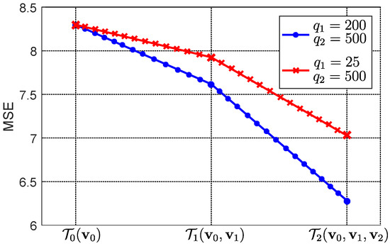
Here, we wish to numerically illustrate Theorems 3, 4, and 5. To this end, we assume that $\mathbf{x}\in L^2(\Omega ,{\mathbb{R}}^m)$ and $\mathbf{y}\in L^2(\Omega ,{\mathbb{R}}^m)$ are uniformly and normally distributed random vectors, respectively. Injections ${\mathbf{v}}_1\in L^2(\Omega ,{\mathbb{R}}^{q_1})$ and ${\mathbf{v}}_2\in L^2(\Omega ,{\mathbb{R}}^{q_2})$ are here chosen as uniformly distributed random vectors. Covariance matrices $E_{x{v}_j}$, $E_{v_i{v}_j}$, for $i,j=0,1,2$, are represented by $E_{x{v}_j}=\frac{1}{s}X{V}_j^{T}and{E}_{v_i{v}_j}=\frac{1}{s}{V}_i{V}_j^T$ where $X\in {\mathbb{R}}^{m\times s}$ and $V_j\in {\mathbb{R}}^{q_j\times s}$ are sample matrices of $\mathbf{x}$ and ${\mathbf{v}}_j$, respectively, for $j=0,1,2$.

We choose $m=100$ and $r=50$. It follows from Theorems 3, 4, and 5 that the error associated with approximating operator ${\mathcal{T}}_p({\mathbf{v}}_0,\dots ,{\mathbf{v}}_p)$ varies if values of p, $q=q_0+\dots +q_p$ and $r=r_0+\dots +r_p$ vary. We wish to illustrate the decrease in error when, for the same r, values of p and q increase. To this end, we provide Table 1 and Table 2, where values of the errors are given for different values of $q_j$, $r_j$, for $j=0,1,2$ and $p=0,1,2$. In Table 1 and Table 2, the abbreviation MSE (mean square error) is used to unite notations ${\epsilon }_{GH}^{(p)}$ and ${\epsilon }_{GH}^{(g)}$ used in Theorems 3, 4, and 5. In the tables, Cases 1 and 2 for specific values of $q_j$, $r_j$ are considered.

Table 1. Numerical characterizations of approximating operators ${\mathcal{T}}_0({\mathbf{v}}_0)$, ${\mathcal{T}}_1({\mathbf{v}}_0,{\mathbf{v}}_1)$, and ${\mathcal{T}}_2({\mathbf{v}}_0,{\mathbf{v}}_1,{\mathbf{v}}_2)$ in Case 1.

Approximating Operator	${\mathit{q}}_0$	${\mathit{q}}_1$	${\mathit{q}}_2$	${\mathit{r}}_0$	${\mathit{r}}_1$	${\mathit{r}}_2$	MSE
${\mathcal{T}}_0({\mathbf{v}}_0)$	100	N/A	N/A	50	N/A	N/A	8.30
${\mathcal{T}}_1({\mathbf{v}}_0,{\mathbf{v}}_1)$	100	25	N/A	25	25	N/A	7.93
${\mathcal{T}}_2({\mathbf{v}}_0,{\mathbf{v}}_1,{\mathbf{v}}_2)$	100	25	500	17	17	16	7.03

Table 2. Numerical characterizations of operators ${\mathcal{T}}_0({\mathbf{v}}_0)$, ${\mathcal{T}}_1({\mathbf{v}}_0,{\mathbf{v}}_1)$, and ${\mathcal{T}}_2({\mathbf{v}}_0,{\mathbf{v}}_1,{\mathbf{v}}_2)$ in Case 2.

Approximating Operator	${\mathit{q}}_0$	${\mathit{q}}_1$	${\mathit{q}}_2$	${\mathit{r}}_0$	${\mathit{r}}_1$	${\mathit{r}}_2$	MSE
${\mathcal{T}}_0({\mathbf{v}}_0)$	100	N/A	N/A	50	N/A	N/A	8.30
${\mathcal{T}}_1({\mathbf{v}}_0,{\mathbf{v}}_1)$	100	200	N/A	25	25	N/A	7.61
${\mathcal{T}}_2({\mathbf{v}}_0,{\mathbf{v}}_1,{\mathbf{v}}_2)$	100	200	500	17	17	16	6.28

In Figure 2 the MSE values are illustrated diagrammatically.

Figure 2. Example 1: Diagrams of the errors associated with ${\mathcal{T}}_0({\mathbf{v}}_0)$, ${\mathcal{T}}_1({\mathbf{v}}_0,{\mathbf{v}}_1)$, and ${\mathcal{T}}_2({\mathbf{v}}_0,{\mathbf{v}}_1,{\mathbf{v}}_2)$.

It follows from Table 1 and Table 2 and Figure 2 that, for the same r, the error associated with the proposed system model decreases if degree p or the sum q of the injection dimensions increases. This is because the increase in the number of parameters to optimize in the operator $\mathcal{T}$ results in a decrease in the error, as stated in Theorem 5.

3.4. Particular Case: No Reduction of Vector Dimensionality

An important particular case of the problem in (16) and (9) is when matrix $G_j{H}_j$ is replaced with a full rank matrix $M_j\in {\mathbb{R}}^{m\times q_j}$, for $j=0,\dots ,h$. Operator ${\mathcal{S}}_h$ given by

$$\begin{array}{c}\hfill {\mathcal{S}}_h({\mathbf{v}}_0,\dots {\mathbf{v}}_p)={\displaystyle \sum _{k=0}^h}{M}_k{\mathbf{z}}_k\end{array}$$

(40)

is called the full rank approximating operator. The problem then is to find matrices $M_0,\dots ,M_h$ that solve

$$\begin{array}{c}\hfill {\displaystyle \underset{M_0,\dots ,M_h}{min}}\parallel \mathcal{F}(\mathbf{y})-{\displaystyle \sum _{k=0}^h}{M}_k{\mathbf{z}}_k{\parallel }_{\Omega }^2,\end{array}$$

(41)

subject to condition (9).

In particular, searched matrices $M_0,\dots ,M_h$ can be found, for $\omega \in \Omega$, from equations

$$\begin{array}{c}\hfill M_j{\mathbf{z}}_j(\omega )=[\mathcal{F}(\mathbf{y})](\omega ),\mathrm{for}j=0,\dots ,h,\end{array}$$

(42)

and

$$\begin{array}{c}\hfill {\displaystyle \sum _{k=0}^h}{M}_k{\mathbf{z}}_k(\omega )=[\mathcal{F}(\mathbf{y})](\omega ),\end{array}$$

(43)

respectively. Those equations may have an infinite number of solutions or have no solutions. Therefore, instead, the following theorem provides the solution to the problem in (41) where cases (42) and (43) are excluded.

Theorem 6.

Let ${\mathbf{v}}_0,\dots ,{\mathbf{v}}_p$ be well-defined injections and vectors ${\mathbf{z}}_0,\dots ,{\mathbf{z}}_p$ be pairwise uncorrelated. Let $\mathcal{F}(\mathbf{y})\ne M_j{\mathbf{z}}_{\mathbf{j}}$, for $j=0,\dots ,h,$ and ${\displaystyle \mathcal{F}(\mathbf{y})\ne {\displaystyle \sum _{k=0}^h}{M}_k{\mathbf{z}}_k}$. Then, the minimal Frobenius norm solution to the problem (41) is given, for $k=0,\dots ,h$, by

$$\begin{array}{c}\hfill M_k=E_{x{z}_k}{E}_{z_k{z}_k}^{†}.\end{array}$$

(44)

Proof. 

Similar to (22),

$$\begin{array}{c}\hfill \parallel \mathcal{F}(\mathbf{y})-{\displaystyle \sum _{j=0}^h}{M}_j{\mathbf{z}}_j{\parallel }_{\Omega }^2={\displaystyle \sum _{j=0}^h}{\parallel \mathbf{x}-M_j{\mathbf{z}}_{\mathbf{j}}\parallel }_{\Omega }^2-\mathrm{tr}\left\{h{E}_{xx}\right\}.\end{array}$$

(45)

It is known (see, for example, [16,20,21]) that the minimal Frobenius norm solution to the problem

$${\displaystyle \underset{M_j}{min}}{\parallel \mathbf{x}-M_j{\mathbf{z}}_{\mathbf{j}}\parallel }_{\Omega }^2$$

is given by (44). □

Theorem 7.

Let $A_j=E_{x{z}_j}{(E_{z_j{z}_j}^{1/2})}^{†}$. The error associated with the minimal Frobenius norm solution to the problem in (41) is represented by

$$\begin{array}{c}\hfill {\displaystyle \underset{M_0,\dots ,M_h}{min}}\parallel \mathcal{F}(\mathbf{y})-{\displaystyle \sum _{j=0}^h}{M}_j{\mathbf{z}}_j{\parallel }_{\Omega }^2=\mathit{tr}\left\{E_{xx}\right\}-{\displaystyle \sum _{j=0}^h}{\parallel A_j\parallel }^2.\end{array}$$

(46)

Proof. 

For $M_j$ determined by (44),

$$\parallel \mathcal{F}(\mathbf{y})-M_j{\mathbf{z}}_j{\parallel }_{\Omega }^2=\mathrm{tr}\left\{E_{xx}\right\}-\parallel E_{x{z}_j}{(E_{z_j{z}_j}^{1/2})}^{†}{\parallel }^2+{\parallel M_j{E}_{z_j{z}_j}^{1/2}-E_{x{z}_j}{(E_{z_j{z}_j}^{1/2})}^{†}\parallel }^2.$$

(47)

Here,

$$\begin{array}{ccc}\hfill \parallel M_j{E}_{z_j{z}_j}^{1/2}-E_{x{z}_j}{(E_{z_j{z}_j}^{1/2})}^{†}{\parallel }^2& =& \parallel E_{x{z}_j}{E}_{z_j{z}_j}^{†}{E}_{z_j{z}_j}^{1/2}-E_{x{z}_j}{(E_{z_j{z}_j}^{1/2})}^{†}{\parallel }^2\hfill \\ & =& \parallel E_{x{z}_j}{(E_{z_j{z}_j}^{1/2})}^{†}-E_{x{z}_j}{(E_{z_j{z}_j}^{1/2})}^{†}{\parallel }^2=0.\hfill \end{array}$$

(48)

That is,

$$\begin{array}{c}\hfill \parallel \mathcal{F}(\mathbf{y})-M_j{\mathbf{z}}_j{\parallel }_{\Omega }^2=\mathrm{tr}\left\{E_{xx}\right\}-{\parallel E_{x{z}_j}{(E_{z_j{z}_j}^{1/2})}^{†}\parallel }^2.\end{array}$$

(49)

Then, (46) follows from (22) and (48). □

4. Solution of Problem Given by (7), (8), (9)

Now we are in the position to consider a solution to the original problem in (7), (8), (9).

4.1. Device of Solution

In comparison with the problem in (16), (8), (9), a specific difficulty of the original problem in (7), (8), (9) is a determination of p additional unknowns, injections ${\mathbf{v}}_1,\dots ,{\mathbf{v}}_p$.

The device of the proposed solution is as follows. First, in (13) and (14), arbitrary linearly independent in the generalized sense vectors ${\mathbf{v}}_0,\dots ,{\mathbf{v}}_p$ are denoted by ${\mathbf{v}}_0^{(0)},\dots ,{\mathbf{v}}_p^{(0)}$ and pairwise uncorrelated random vectors ${\mathbf{z}}_0,\dots ,{\mathbf{z}}_p$ are denoted by ${\mathbf{z}}_0({\mathbf{v}}_0^{(0)}),$ $\dots ,$ ${\mathbf{z}}_p({\mathbf{v}}_p^{(0)})$. In (19), matrices $G_j$ and $H_j$, for $j=0,\dots ,p$, are denoted by $G_j^{(0)}$ and $H_j^{(0)}$, respectively. The associated error is still represented by (27). We also write

$$\begin{array}{c}\hfill {\epsilon }^{(0)}=\parallel \mathcal{F}(\mathbf{y})-{\displaystyle \sum _{k=0}^p}{G}_k^{(0)}{H}_k^{(0)}{\mathbf{z}}_k({\mathbf{v}}_k^{(0)}){\parallel }_{\Omega }^2.\end{array}$$

(50)

Then, for $i=0,1,\dots$, searched injections ${\mathbf{v}}_1^{(i+1)},$ $\dots ,{\mathbf{v}}_p^{(i+1)}$ and matrices $G_1^{(i+1)},$ $H_1^{(i+1)}$, $\dots G_p^{(i+1)},H_p^{(i+1)}$ are determined by the iterative procedure represented bellow. It will be shown in Theorem 10 below that ${\mathbf{v}}_1^{(i+1)},$ $\dots ,{\mathbf{v}}_p^{(i+1)}$ and $G_1^{(i+1)},$ $H_1^{(i+1)}$, $\dots G_p^{(i+1)},H_p^{(i+1)}$ further minimize the associated error. The i-th iterative loop of the iterative procedure consists of the steps as follows.

The i-th iterative loop, for $i=0,1,\dots .$

Step 1. Given ${\mathbf{v}}_0=\mathbf{y}$, $G_0^{(i)},H_0^{(i)},\dots ,$ $G_p^{(i)},H_p^{(i)}$, find ${\mathbf{v}}_1,\dots ,{\mathbf{v}}_p$ that solve

$$\begin{array}{c}\hfill {\displaystyle \underset{{\mathbf{v}}_1,\dots ,{\mathbf{v}}_p}{min}}\parallel \mathcal{F}(\mathbf{y})-{\displaystyle \sum _{k=1}^p}{G}_k^{(i)}{H}_k^{(i)}{\mathbf{z}}_k({\mathbf{v}}_k){\parallel }_{\Omega }^2,\end{array}$$

(51)

where

$$\begin{array}{c}\hfill {\displaystyle {\mathbf{z}}_j({\mathbf{v}}_j)={\mathbf{v}}_j-{\displaystyle \sum _{k=0}^{j-1}}{E}_{v_j{z}_k(v_k)}{E}_{z_k(v_k)z_k(v_k)}^{†}{\mathbf{z}}_k({\mathbf{v}}_k).}\end{array}$$

(52)

The solution is denoted by ${\mathbf{v}}_1^{(i+1)},\dots ,{\mathbf{v}}_p^{(i+1)}$. We call ${\mathbf{v}}_1^{(i+1)},\dots ,{\mathbf{v}}_p^{(i+1)}$ the optimal injections.

Step 2. Given ${\mathbf{v}}_1^{(i+1)},\dots ,{\mathbf{v}}_p^{(i+1)}$, find pairwise uncorrelated random vectors ${\mathbf{z}}_1({\mathbf{v}}_1^{(i+1)}),$ $\dots ,{\mathbf{z}}_p({\mathbf{v}}_p^{(i+1)})$ and denote

$$\begin{array}{c}\hfill {\epsilon }_v^{(i+1)}=\parallel \mathcal{F}(\mathbf{y})-{\displaystyle \sum _{k=0}^p}{G}_k^{(i)}{H}_k^{(i)}{\mathbf{z}}_k({\mathbf{v}}_k^{(i+1)}){\parallel }_{\Omega }^2,\end{array}$$

(53)

where, for $k=0$, we set $G_0^{(i)}=G_0^{(0)}$ and $H_0^{(i)}=H_0^{(0)}$, for all $i=1,2,\dots$ and we write

$$\begin{array}{c}\hfill {\displaystyle {\mathbf{z}}_j({\mathbf{v}}_j^{(i)})={\mathbf{v}}_j^{(i)}-{\displaystyle \sum _{k=0}^{j-1}}{E}_{v_j^{(i)}{z}_k(v_k^{(i)})}{E}_{z_k(v_k^{(i)})z_k(v_k^{(i)})}^{†}{\mathbf{z}}_k({\mathbf{v}}_k^{(i)}).}\end{array}$$

(54)

Step 3. Given ${\mathbf{z}}_1({\mathbf{v}}_1^{(i)}),\dots ,{\mathbf{z}}_p({\mathbf{v}}_p^{(i)})$, find $G_1,H_1,\dots ,G_p,H_p$ that solve

$$\begin{array}{c}\hfill {\displaystyle \underset{\begin{array}{c}{G}_1,H_1,\dots ,G_p,H_p\end{array}}{min}}{∥\mathcal{F}(\mathbf{y})-{\displaystyle \sum _{k=1}^p}{G}_k{H}_k{\mathbf{z}}_k({\mathbf{v}}_k^{(i)})∥}_{\Omega }^2.\end{array}$$

(55)

The solution of problem (55) is denoted by $G_1^{(i+1)},H_1^{(i+1)},\dots ,$ $G_p^{(i+1)},H_p^{(i+1)}$. Further, denote

$$\begin{array}{c}\hfill {\epsilon }_{GH}^{(i+1)}=\parallel \mathcal{F}(\mathbf{y})-{\displaystyle \sum _{k=0}^p}{G}_k^{(i+1)}{H}_k^{(i+1)}{\mathbf{z}}_k({\mathbf{v}}_k^{(i)}){\parallel }_{\Omega }^2,\end{array}$$

(56)

where, as before, for $k=0$, we set $G_0^{(i+1)}=G_0^{(0)}$ and $H_0^{(i+1)}=H_0^{(0)}$, for all $i=0,1,\dots$.

Step 4. Denote

$$\begin{array}{c}\hfill {\epsilon }^{(i+1)}=min\{{\epsilon }_v^{(i+1)},{\epsilon }_{GH}^{(i+1)}\}.\end{array}$$

(57)

Step 5. If, for a given tolerance $\mathit{\delta }$,

$$\begin{array}{c}\hfill \parallel {\epsilon }^{(i+1)}-{\epsilon }^{(i)}{\parallel }_{\Omega }^2\le \mathit{\delta },\end{array}$$

(58)

the iterations are stopped. If not, then Steps 1–4 are repeated to form the next iterative loop.

The above steps of the solution device are consummated as follows.

4.2. Determination of ${\mathbf{v}}_j^{(i+1)}$ in Step 1

Let us denote

$$\begin{array}{ccc}\hfill & & {\mathbf{z}}_k^{(i+1)}={\mathbf{z}}_k({\mathbf{v}}_k^{(i+1)}),P_j^{(i)}=G_j^{(i)}{H}_j^{(i)},B_{jk}^{(i+1)}={(P_j^{(i)})}^{†}{E}_{x{z}_k^{(i+1)}},\hfill \\ & & {\mathbf{\gamma }}_{\mathit{\ell }}^{(i+1)}=E_{z_{\mathit{\ell }}^{(i+1)}{z}_{\mathit{\ell }}^{(i+1)}}^{†}{\mathbf{z}}_{\mathit{\ell }}^{(i+1)}\mathrm{and}{A}_{\mathit{\ell }k}^{(i+1)}=E_{z_{\mathit{\ell }}^{(i+1)}{z}_{\mathit{\ell }}^{(i+1)}}^{†}{E}_{z_{\mathit{\ell }}^{(i+1)}{z}_k^{(i+1)}}.\hfill \end{array}$$

Here, ${\mathbf{\gamma }}_{\mathit{\ell }}^{(i+1)}(\omega )\in {\mathbb{R}}^{q_{\mathit{\ell }}\times q_{\mathit{\ell }}}$, $B_{jk}^{(i+1)}\in {\mathbb{R}}^{q_j\times q_k}$ and $A_{\mathit{\ell }k}^{(i+1)}\in {\mathbb{R}}^{q_{\mathit{\ell }}\times q_k}$.

Theorem 8.

Let

$$\begin{array}{c}\hfill B_j^{(i)}=[B_{j0}^{(i)},\dots ,B_{j,j-1}^{(i)}]and{A}_j^{(i)}={\left\{A_{ks}^{(i)}\right\}}_{k,s=0}^{j-1},\end{array}$$

(59)

where $B_j^{(i)}\in {\mathbb{R}}^{q_j\times q}$, $A_j^{(i)}\in {\mathbb{R}}^{q\times q}$ and $q=q_0+\dots +q_{j-1}$. Then the optimal injection ${\mathbf{v}}_j^{(i+1)}$, for $j=1,\dots ,p$, that solves the problem in (51) is determined by

$$\begin{array}{c}\hfill {\mathbf{v}}_j^{(i+1)}(\omega )={(G_j^{(i)}{H}_j^{(i)})}^{†}[\mathcal{F}(\mathbf{y})](\omega )+{\displaystyle \sum _{\mathit{\ell }=0}^{j-1}}{C}_{j\mathit{\ell }}^{(i)}{\mathbf{\gamma }}_{\mathit{\ell }}^{(i)}(\omega ),\end{array}$$

(60)

where matrices $C_{j0}^{(i)},\dots ,C_{j,j-1}^{(i)}$ are defined by

$$\begin{array}{c}\hfill [C_{j0}^{(i)},\dots ,C_{j,j-1}^{(i)}]=B_j^{(i)}{(I-A_j^{(i)})}^{†}.\end{array}$$

(61)

Here, $C_{j\mathit{\ell }}^{(i)}\in {\mathbb{R}}^{q_j\times q_{\mathit{\ell }}}$, for $\mathit{\ell }=0,\dots ,j-1$.

Proof. 

Based on (22), the problem in (51) is represented as follows:

$$\begin{array}{ccc}\hfill & & {\displaystyle \underset{{\mathbf{v}}_1,\dots ,{\mathbf{v}}_p}{min}}{∥\mathcal{F}(\mathbf{y})-{\displaystyle \sum _{j=0}^p}{P}_j^{(i)}{\mathbf{z}}_j({\mathbf{v}}_j)∥}_{\Omega }^2={∥\mathcal{F}(\mathbf{y})-P_0^{(0)}{\mathbf{z}}_0({\mathbf{v}}_0)∥}_{\Omega }^2\hfill \\ & & +{\displaystyle \sum _{j=1}^p}{\displaystyle \underset{{\mathbf{v}}_j}{min}}{∥\mathcal{F}(\mathbf{y})-P_j^{(i)}{\mathbf{z}}_j({\mathbf{v}}_j)∥}_{\Omega }^2-\mathrm{tr}\left\{p{E}_{xx}\right\}.\hfill \end{array}$$

(62)

Then

$$\begin{array}{ccc}\hfill {\displaystyle \underset{{\mathbf{v}}_j}{min}}{∥\mathcal{F}(\mathbf{y})-P_j^{(i)}{\mathbf{z}}_j({\mathbf{v}}_j)∥}_{\Omega }^2& =& {\displaystyle \underset{{\mathbf{v}}_j}{min}}{∥\mathcal{F}(\mathbf{y})-P_j^{(i)}\left({\mathbf{v}}_j-{\displaystyle \sum _{k=0}^{j-1}}{E}_{v_j{z}_k}{E}_{z_k{z}_k}^{†}{\mathbf{z}}_k({\mathbf{v}}_k)\right)∥}_{\Omega }^2.\hfill \end{array}$$

(63)

Here,

$$\begin{array}{ccc}\hfill & & {∥\mathcal{F}(\mathbf{y})-P_j^{(i)}\left({\mathbf{v}}_j-{\displaystyle \sum _{k=0}^{j-1}}{E}_{v_j{z}_k}{E}_{z_k{z}_k}^{†}{\mathbf{z}}_k({\mathbf{v}}_k)\right)∥}_{\Omega }^2\hfill \\ & =& {\int }_{\Omega }{∥[\mathcal{F}(\mathbf{y})](\omega )-P_j^{(i)}\left({\mathbf{v}}_j(\omega )-{\displaystyle \sum _{k=0}^{j-1}}{E}_{v_j{z}_k}{E}_{z_k{z}_k}^{†}{\mathbf{z}}_k({\mathbf{v}}_k(\omega ))\right)∥}^{2}d\mathit{\mu }(\omega )\hfill \\ & =& {\int }_{\Omega }{∥[\mathcal{F}(\mathbf{y})](\omega )-P_j^{(i)}{\mathbf{z}}_j({\mathbf{v}}_j(\omega ))∥}^{2}d\mathit{\mu }(\omega ).\hfill \end{array}$$

(64)

For $\mathbf{u}={\mathbf{z}}_j(({\mathbf{v}}_j),$ let us denote ${\mathcal{U}}_v=\{\mathbf{u}\in L^2(\Omega ,{\mathbb{R}}^{q_j})\mid \mathbf{u}={\mathbf{z}}_j(({\mathbf{v}}_j)\}$. For any $\mathbf{u}$, let us write $\mathcal{U}=\{\mathbf{u}\in L^2(\Omega ,{\mathbb{R}}^{q_j})\}.$ For $j=1,\dots ,p$, the vector $\tilde{\mathbf{u}}(\omega )\in {\mathbb{R}}^{q_j}$ of the smallest Euclidean norm of all minimizers that solves

$${\displaystyle \underset{\mathbf{u}(\omega )}{min}}\parallel [\mathcal{F}(\mathbf{y})](\omega )-P_j^{(i)}{\mathbf{u}(\omega )\parallel }^2$$

is given by (see [85], p. 257)

$$\begin{array}{c}\hfill \tilde{\mathbf{u}}(\omega )={(P_j^{(i)})}^{†}[\mathcal{F}(\mathbf{y})](\omega ).\end{array}$$

Let ${\mathbf{v}}_j^{(i+1)}$ be such that

$${\displaystyle \underset{{\mathbf{v}}_j(\omega )}{min}}\parallel [\mathcal{F}(\mathbf{y})](\omega )-P_j^{(i)}{\mathbf{z}}_j({\mathbf{v}}_j(\omega )){\parallel }^2=\parallel [\mathcal{F}(\mathbf{y})](\omega )-P_j^{(i)}{\mathbf{z}}_j({\mathbf{v}}_j^{(i+1)}(\omega )){\parallel }^2.$$

Since ${\mathcal{U}}_v\subset \mathcal{U}$ then

$$\begin{array}{c}\hfill {\displaystyle \underset{{\mathbf{v}}_j(\omega )}{min}}\parallel [\mathcal{F}(\mathbf{y})](\omega )-P_j^{(i)}{\mathbf{z}}_j({\mathbf{v}}_j(\omega )){\parallel }^2\ge {\displaystyle \underset{\mathbf{u}(\omega )}{min}}\parallel [\mathcal{F}(\mathbf{y})](\omega )-P_j^{(i)}{\mathbf{u}(\omega )\parallel }^2,\end{array}$$

(65)

i.e.,

$$\begin{array}{ccc}\hfill {\displaystyle \underset{{\mathbf{v}}_j(\omega )}{min}}\parallel [\mathcal{F}(\mathbf{y})](\omega )-P_j^{(i)}{\mathbf{z}}_j({\mathbf{v}}_j(\omega )){\parallel }^2& \ge & \parallel [\mathcal{F}(\mathbf{y})](\omega )-P_j^{(i)}\tilde{\mathbf{u}}{(\omega )\parallel }^2\hfill \\ & =& \parallel [\mathcal{F}(\mathbf{y})](\omega )-P_j^{(i)}{(P_j^{(i)})}^{†}[\mathcal{F}(\mathbf{y}){](\omega )\parallel }^2\hfill \end{array}$$

(66)

Then (66) implies that, for all ${\mathbf{v}}_j$,

$$\begin{array}{c}\hfill \parallel [\mathcal{F}(\mathbf{y})](\omega )-P_j^{(i)}{\mathbf{z}}_j({\mathbf{v}}_j(\omega )){\parallel }^2\ge \parallel [\mathcal{F}(\mathbf{y})](\omega )-P_j^{(i)}{(P_j^{(i)})}^{†}[\mathcal{F}(\mathbf{y}){](\omega )\parallel }^2.\end{array}$$

(67)

Since it is true for all ${\mathbf{v}}_j$, then

$$\begin{array}{c}\hfill \parallel [\mathcal{F}(\mathbf{y})](\omega )-P_j^{(i)}{(P_j^{(i)})}^{†}[\mathcal{F}(\mathbf{y})](\omega ){\parallel }^2={\displaystyle \underset{{\mathbf{v}}_j(\omega )}{min}}\parallel [\mathcal{F}(\mathbf{y}){](\omega )-P_j^{(i)}{\mathbf{z}}_j({\mathbf{v}}_j(\omega ))\parallel }^2,\end{array}$$

(68)

i.e.,

$$\parallel [\mathcal{F}(\mathbf{y})](\omega )-P_j^{(i)}{(P_j^{(i)})}^{†}[\mathcal{F}(\mathbf{y})](\omega ){\parallel }^2=\parallel [\mathcal{F}(\mathbf{y}){](\omega )-P_j^{(i)}{\mathbf{z}}_j({\mathbf{v}}_j^{(i+1)}(\omega ))\parallel }^2.$$

Therefore,

$$\begin{array}{c}\hfill {\mathbf{z}}_j({\mathbf{v}}_j^{(i+1)}(\omega ))={(P_j^{(i)})}^{†}[\mathcal{F}(\mathbf{y})](\omega ).\end{array}$$

(69)

Taking into account (14), Equation (69) is written as

$${\displaystyle {\mathbf{v}}_j^{(i+1)}(\omega )={(P_j^{(i)})}^{†}[\mathcal{F}(\mathbf{y})](\omega )+{\displaystyle \sum _{k=0}^{j-1}}{E}_{v_j^{(i+1)}{z}_k^{(i+1)}}{E}_{z_k^{(i+1)}{z}_k^{(i+1)}}^{†}{\mathbf{z}}_k({\mathbf{v}}_k^{(i+1)}(\omega )),}$$

where we denote

$$\begin{array}{ccc}& & {\displaystyle E_{v_j^{(i+1)}{z}_k^{(i+1)}}={\int }_{\Omega }{\mathbf{v}}_j^{(i+1)}(\xi ){\mathbf{z}}_k{\left[{\mathbf{v}}_k^{(i+1)}(\xi )\right]}^{T}d\mathit{\mu }(\xi ),}\hfill \\ & & {\displaystyle \mathrm{and}{E}_{z_k^{(i+1)}{z}_k^{(i+1)}}={\int }_{\Omega }{\mathbf{z}}_k\left[{\mathbf{v}}_k^{(i+1)}(\xi )\right]{\mathbf{z}}_k{\left[{\mathbf{v}}_k^{(i+1)}(\xi )\right]}^{T}d\mathit{\mu }(\xi ).}\hfill \end{array}$$

Thus,

$$\begin{array}{c}\hfill {\mathbf{v}}_j^{(i+1)}(\omega )={(P_j^{(i)})}^{†}[\mathcal{F}(\mathbf{y})](\omega )+{\displaystyle \sum _{\mathit{\ell }=0}^{j-1}}\left[{\int }_{\Omega }{\mathbf{v}}_j^{(i+1)}(\xi ){\left[{\mathbf{z}}_{\mathit{\ell }}({\mathbf{v}}_{\mathit{\ell }}^{(i+1)}(\xi ))\right]}^{T}d\mathit{\mu }(\xi )\right]{\mathbf{\gamma }}_{\mathit{\ell }}^{(i+1)}(\omega ).\end{array}$$

(70)

Let us now write Equation (70) as follows:

$$\begin{array}{c}\hfill {\mathbf{v}}_j^{(i+1)}(\omega )={\mathbf{\alpha }}_j^{(i)}(\omega )+{\int }_{\Omega }{K}_j^{(i+1)}(\omega ,\xi ){\mathbf{v}}_j^{(i+1)}(\xi )d\mathit{\mu }(\xi ),\end{array}$$

(71)

where

$$\begin{array}{c}\hfill {\displaystyle {\mathbf{\alpha }}_j^{(i)}(\omega )={(P_j^{(i)})}^{†}[\mathcal{F}(\mathbf{y})](\omega )\mathrm{and}{K}_j^{(i+1)}(\omega ,\xi )={\displaystyle \sum _{\mathit{\ell }=0}^{j-1}}{\left[{\mathbf{z}}_{\mathit{\ell }}({\mathbf{v}}_{\mathit{\ell }}^{(i+1)}(\xi ))\right]}^T{\mathbf{\gamma }}_{\mathit{\ell }}^{(i+1)}(\omega ).}\end{array}$$

(72)

Recall that in (72), matrix $P_j^{(i)}=G_j^{(i)}{H}_j^{(i)}$ depends on ${\mathbf{v}}_j^{(i)}(\omega )$, not on ${\mathbf{v}}_j^{(i+1)}(\omega )$. Therefore, Equation (71) is a vector version of the Fredholm integral equation of the second kind [86] with respect to ${\mathbf{v}}_j^{(i+1)}(\omega )$. Its solution is provided as follows. Write Equation (71) as

$$\begin{array}{c}\hfill {\mathbf{v}}_j^{(i+1)}(\omega )={\mathbf{\alpha }}_j^{(i)}(\omega )+{\displaystyle \sum _{\mathit{\ell }=0}^{j-1}}{C}_{j\mathit{\ell }}^{(i+1)}{\mathbf{\gamma }}_{\mathit{\ell }}^{(i+1)}(\omega ),\end{array}$$

(73)

where

$${\displaystyle C_{j\mathit{\ell }}^{(i+1)}={\int }_{\Omega }{\mathbf{v}}_j^{(i+1)}(\xi ){\left[{\mathbf{z}}_{\mathit{\ell }}({\mathbf{v}}_{\mathit{\ell }}^{(i+1)}(\xi ))\right]}^{T}d\mathit{\mu }(\xi ).}$$

Let us now multiply both sides of (73) by ${\left[{\mathbf{z}}_k({\mathbf{v}}_k^{(i+1)}(\omega ))\right]}^T$, for $k=0,\dots ,j-1$, and integrate. It implies

$$\begin{array}{ccc}\hfill {\int }_{\Omega }{\mathbf{v}}_j^{(i+1)}(\omega ){\left[{\mathbf{z}}_k({\mathbf{v}}_k^{(i+1)}(\omega ))\right]}^{T}d\mathit{\mu }(\omega )& =& {\int }_{\Omega }{\mathbf{\alpha }}_j^{(i)}(\omega ){\left[{\mathbf{z}}_k({\mathbf{v}}_k^{(i+1)}(\omega ))\right]}^{T}d\mathit{\mu }(\omega )\hfill \\ & & +{\displaystyle \sum _{\mathit{\ell }=0}^{j-1}}{C}_{j\mathit{\ell }}^{(i+1)}{\int }_{\Omega }{\mathbf{\gamma }}_{\mathit{\ell }}^{(i+1)}(\omega ){\left[{\mathbf{z}}_k({\mathbf{v}}_k^{(i+1)}(\omega ))\right]}^{T}d\mathit{\mu }(\omega )\hfill \end{array}$$

and

$$\begin{array}{c}\hfill C_{jk}^{(i+1)}=B_{jk}^{(i+1)}+{\displaystyle \sum _{\mathit{\ell }=0}^{j-1}}{C}_{j\mathit{\ell }}^{(i+1)}{A}_{\mathit{\ell }k}^{(i+1)},\end{array}$$

(74)

where, for $k=0,\dots ,j-1$,

$$\begin{array}{ccc}\hfill B_{jk}^{(i+1)}& =& {\int }_{\Omega }{\mathbf{\alpha }}_j^{(i+1)}(\omega ){\left[{\mathbf{z}}_k({\mathbf{v}}_k^{(i+1)}(\omega ))\right]}^{T}d\mathit{\mu }(\omega )\hfill \\ & =& {(P_j^{(i)})}^{†}{\int }_{\Omega }[\mathcal{F}(\mathbf{y})](\omega ){\left[{\mathbf{z}}_k({\mathbf{v}}_k^{(i+1)}(\omega ))\right]}^{T}d\mathit{\mu }(\omega )={(P_j^{(i)})}^{†}{E}_{x{z}_k^{(i+1)}}\in {\mathbb{R}}^{q_j\times q_k}\hfill \end{array}$$

and

$$\begin{array}{c}\hfill A_{\mathit{\ell }k}^{(i+1)}={\int }_{\Omega }{\mathbf{\gamma }}_{\mathit{\ell }}^{(i+1)}(\omega ){\left[{\mathbf{z}}_k({\mathbf{v}}_k^{(i+1)}(\omega ))\right]}^{T}d\mathit{\mu }(\omega )=E_{z_{\mathit{\ell }}^{(i+1)}{z}_{\mathit{\ell }}^{(i+1)}}^{†}{E}_{z_{\mathit{\ell }}^{(i+1)}{z}_k^{(i+1)}}\in {\mathbb{R}}^{q_{\mathit{\ell }}\times q_k}.\end{array}$$

Let $C_j^{(i+1)}=[C_{j0}^{(i+1)},\dots ,C_{j,j-1}^{(i+1)}]\in {\mathbb{R}}^{q_j\times q}$. Then the set of matrix equations in (74) can be written as a single equation

$$\begin{array}{c}\hfill C_j^{(i+1)}=B_j^{(i+1)}+C_j^{(i+1)}{A}_j^{(i+1)}\mathrm{or}{B}_j^{(i+1)}=C_j^{(i+1)}(I-A_j^{(i+1)}).\end{array}$$

(75)

If matrix $I-A_j^{(i+1)}$ is invertible, then (75) implies

$$\begin{array}{c}\hfill C_j^{(i+1)}=B_j^{(i+1)}{(I-A_j^{(i+1)})}^{-1}.\end{array}$$

(76)

If matrix $I-A_j^{(i+1)}$ is singular, then instead of Equation (75), we consider the problem

$$\begin{array}{c}\hfill {\displaystyle \underset{C_j^{(i+1)}}{min}}{\parallel B_j^{(i+1)}-C_j^{(i+1)}(I-A_j^{(i+1)})\parallel }^2.\end{array}$$

(77)

Its minimal Frobenius norm solution is given by [62]:

$$\begin{array}{c}\hfill C_j^{(i+1)}=B_j^{(i+1)}{(I-A_j^{(i+1)})}^{†}.\end{array}$$

(78)

Thus, injection ${\mathbf{v}}_j^{(i+1)}$ follows from (73), (76), and (78). □

In terms of a multilayer network, this procedure is illustrated diagrammatically in Figure 1. To simplify the notation, superscripts $(i)$ and $(i+1)$ are omitted in Figure 1.

4.3. Determination of Matrices $G_1^{(i+1)},H_1^{(i+1)},\dots ,$ $G_p^{(i+1)},H_p^{(i+1)}$ in Step 3

In Step 3, the matrices $G_1^{(i+1)},H_1^{(i+1)},\dots ,$ $G_p^{(i+1)},H_p^{(i+1)}$ solve problem (55). At the same time, the problems in (16) and (55) differ in notation only. Therefore, in Step 3, matrices $G_1^{(i+1)},H_1^{(i+1)},\dots ,$ $G_p^{(i+1)},H_p^{(i+1)}$ are determined, in fact, by Theorem 2, where only the notation should be changed.

Nevertheless, to avoid any confusion, we below provide Theorem 9, where matrices $G_1^{(i+1)},H_1^{(i+1)},\dots ,$ $G_p^{(i+1)},H_p^{(i+1)}$ are represented. To this end, we denote ${\Gamma }_{z_j^{(i)}}=E_{x{z}_j^{(i)}}{E}_{z_j^{(i)}{z}_j^{(i)}}^{†}{E}_{z_j^{(i)}x}$. To simplify the notation, we set ${\Gamma }_{z_j}:={\Gamma }_{z_j^{(i)}}.$

Theorem 9.

Let ${\mathbf{v}}_0,{\mathbf{v}}_1^{(i)},\dots ,{\mathbf{v}}_p^{(i)}$ be well-defined injections and let vectors ${\mathbf{z}}_1^{(i)},$ $\dots ,{\mathbf{z}}_p^{(i)}$ be pairwise uncorrelated. Then, the minimal Frobenius norm solution to the problem in (55) is given, for $j=1,\dots ,p$, by

$$\begin{array}{c}\hfill G_j^{(i+1)}=U_{{\Gamma }_{z_j},r_j}and{H}_j^{(i+1)}=U_{{\Gamma }_{z_j},r_j}^T{E}_{x{z}_j^{(i)}}{E}_{z_j^{(i)}{z}_j^{(i)}}^{†}.\end{array}$$

(79)

Proof. 

The proof follows from the proof of Theorem 2. □

4.4. Error Analysis of the Solution of Problem in (7), (8), (9)

Theorem 10.

Let $G_0^{(0)},$ $H_0^{(0)},$ $G_k^{(i)},$ $H_k^{(i)}$, and ${\mathbf{v}}_k^{(i)}$, for $k=1,\dots ,p$, $i=0,1,\dots ,$ be determined by Theorems 2, 8, and 9. Let ${\epsilon }^{(i)}$ be the associated error defined by (50) and (57). Then, the increase in the number of iterations i of the procedure represented in nm33,jkw8,nmwk1 implies the decrease in the associated error, i.e.,

$$\begin{array}{c}\hfill {\epsilon }^{(i+1)}\le {\epsilon }^{(i)}.\end{array}$$

(80)

Proof. 

Let us consider the initial case of the proposed technique when $i=0$.

• The case $\mathit{i}=0$. For $i=0$, the i-th iteration loop represented in Section 4.1 implies

  $${\epsilon }_v^{(1)}={\displaystyle \underset{{\mathbf{v}}_1,\dots ,{\mathbf{v}}_p}{min}}\parallel \mathcal{F}(\mathbf{y})-{\displaystyle \sum _{k=1}^p}{G}_k^{(0)}{H}_k^{(0)}{\mathbf{z}}_k({\mathbf{v}}_k){\parallel }_{\Omega }^2.$$
  Here, for $j=1,\dots ,p,$ $G_j^{(1)}=G_j^{(0)}$ and $H_j^{(1)}=H_j^{(0)}$. Therefore,

  $${\epsilon }_v^{(1)}={\displaystyle \underset{{\mathbf{v}}_1,\dots ,{\mathbf{v}}_p}{min}}\parallel \mathcal{F}(\mathbf{y})-{\displaystyle \sum _{k=1}^p}{G}_k^{(1)}{H}_k^{(1)}{\mathbf{z}}_k({\mathbf{v}}_k){\parallel }_{\Omega }^2,$$

  i.e., for any ${\mathbf{v}}_j$, in particular, for ${\mathbf{v}}_j={\mathbf{v}}_j^{(0)}$,

  $$\begin{array}{c}\hfill {\epsilon }_v^{(1)}\le \parallel \mathcal{F}(\mathbf{y})-{\displaystyle \sum _{k=1}^p}{G}_k^{(1)}{H}_k^{(1)}{\mathbf{z}}_k({\mathbf{v}}_k^{(0)}){\parallel }_{\Omega }^2={\epsilon }_{GH}^{(1)}\end{array}$$

  (81)

  and

  $$\begin{array}{c}\hfill {\epsilon }_v^{(1)}\le \parallel \mathcal{F}(\mathbf{y})-{\displaystyle \sum _{k=1}^p}{G}_k^{(0)}{H}_k^{(0)}{\mathbf{z}}_k({\mathbf{v}}_k^{(0)}){\parallel }_{\Omega }^2={\epsilon }^{(0)}.\end{array}$$

  (82)
  Taking into account (81), we denote

  $$\begin{array}{c}\hfill {\epsilon }^{(1)}={\epsilon }_v^{(1)}.\end{array}$$

  (83)
  Then, by (82),

  $$\begin{array}{c}\hfill {\epsilon }^{(1)}\le {\epsilon }^{(0)}.\end{array}$$

  (84)
  For $i=1,2,\dots ,$ let us prove inequality (80) by induction. To this end, we first consider the basis step of the induction, which consists of cases $i=1$ and $i=2$.
• The basis step: Case $\mathit{i}=1$. If $i=1$ then the i-th iteration loop (see Section 4.1) implies

  $$\begin{array}{ccc}\hfill {\epsilon }_{GH}^{(2)}& =& {\displaystyle \underset{\begin{array}{c}{G}_1,H_1,\dots ,G_p,H_p\end{array}}{min}}{∥\mathcal{F}(\mathbf{y})-{\displaystyle \sum _{k=1}^p}{G}_k{H}_k{\mathbf{z}}_k({\mathbf{v}}_k^{(1)})∥}_{\Omega }^2\hfill \\ & =& {∥\mathcal{F}(\mathbf{y})-{\displaystyle \sum _{k=1}^p}{G}_k^{(2)}{H}_k^{(2)}{\mathbf{z}}_k({\mathbf{v}}_k^{(1)})∥}_{\Omega }^2,\hfill \end{array}$$

  i.e., for all $G_k$ and $H_k$ with $k=1,\dots ,p$,

  $${\epsilon }_{GH}^{(2)}\le {∥\mathcal{F}(\mathbf{y})-{\displaystyle \sum _{k=1}^p}{G}_k{H}_k{\mathbf{z}}_k({\mathbf{v}}_k^{(1)})∥}_{\Omega }^2.$$
  In particular, for $G_k=G_k^{(1)}$ and $H_k=H_k^{(1)}$ with $k=1,\dots ,p$,

  $$\begin{array}{c}\hfill {\epsilon }_{GH}^{(2)}\le {∥\mathcal{F}(\mathbf{y})-{\displaystyle \sum _{k=1}^p}{G}_k^{(1)}{H}_k^{(1)}{\mathbf{z}}_k({\mathbf{v}}_k^{(1)})∥}_{\Omega }^2.\end{array}$$

  (85)
  Further, because for $k=1,\dots ,p,$ $G_k^{(1)}=G_k^{(0)}$ and $H_k^{(1)}=H_k^{(0)}$, then

  $$\begin{array}{c}\hfill {\displaystyle \underset{{\mathbf{v}}_1,\dots ,{\mathbf{v}}_p}{min}}\parallel \mathcal{F}(\mathbf{y})-{\displaystyle \sum _{k=1}^p}{G}_k^{(1)}{H}_k^{(1)}{\mathbf{z}}_k({\mathbf{v}}_k){\parallel }_{\Omega }^2={\displaystyle \underset{{\mathbf{v}}_1,\dots ,{\mathbf{v}}_p}{min}}\parallel \mathcal{F}(\mathbf{y})-{\displaystyle \sum _{k=1}^p}{G}_k^{(0)}{H}_k^{(0)}{\mathbf{z}}_k({\mathbf{v}}_k){\parallel }_{\Omega }^2.\end{array}$$

  (86)
  Therefore, for $k=1,\dots ,p$,

  $$\begin{array}{c}\hfill {\mathbf{v}}_k^{(2)}={\mathbf{v}}_k^{(1)}\mathrm{and}{\mathbf{z}}_k({\mathbf{v}}_k^{(2)})={\mathbf{z}}_k({\mathbf{v}}_k^{(1)})\end{array}$$

  (87)
  (see (51)). Thus, (85) and (87) imply

  $$\begin{array}{c}\hfill {\epsilon }_{GH}^{(2)}\le {∥\mathcal{F}(\mathbf{y})-{\displaystyle \sum _{k=1}^p}{G}_k^{(1)}{H}_k^{(1)}{\mathbf{z}}_k({\mathbf{v}}_k^{(2)})∥}_{\Omega }^2={\epsilon }_v^{(2)}.\end{array}$$

  (88)
  But since $G_k^{(1)}=G_k^{(0)}$, $H_k^{(1)}=H_k^{(0)}$ and ${\mathbf{z}}_k({\mathbf{v}}_k^{(2)})={\mathbf{z}}_k({\mathbf{v}}_k^{(1)})$, for $k=1,\dots ,p$, then

  $$\begin{array}{c}\hfill {\epsilon }_v^{(2)}={\epsilon }_v^{(1)}.\end{array}$$

  (89)
  Then by (83), (88), and (89),

  $$\begin{array}{c}\hfill {\epsilon }_{GH}^{(2)}\le {\epsilon }_v^{(1)}={\epsilon }^{(1)}.\end{array}$$

  (90)
  Taking into account (88), we denote

  $$\begin{array}{c}\hfill {\epsilon }^{(2)}={\epsilon }_{GH}^{(2)}.\end{array}$$

  (91)
  Then, (90) and (91) imply

  $$\begin{array}{c}\hfill {\epsilon }^{(2)}\le {\epsilon }^{(1)}.\end{array}$$

  (92)
• The basis step: Case $\mathit{i}=2$. In this case, ${\epsilon }_v^{(i+1)}$ in (53) is written as

  $${\epsilon }_v^{(3)}={\displaystyle \underset{{\mathbf{v}}_1,\dots ,{\mathbf{v}}_p}{min}}\parallel \mathcal{F}(\mathbf{y})-{\displaystyle \sum _{k=0}^p}{G}_k^{(2)}{H}_k^{(2)}{\mathbf{z}}_k({\mathbf{v}}_k){\parallel }_{\Omega }^2=\parallel \mathcal{F}(\mathbf{y})-{\displaystyle \sum _{k=1}^p}{G}_k^{(2)}{H}_k^{(2)}{\mathbf{z}}_k({\mathbf{v}}_k^{(3)}){\parallel }_{\Omega }^2.$$
  That is, for any ${\mathbf{v}}_1,\dots ,{\mathbf{v}}_p,$

  $$\begin{array}{c}\hfill {\epsilon }_v^{(3)}\le \parallel \mathcal{F}(\mathbf{y})-{\displaystyle \sum _{k=0}^p}{G}_k^{(2)}{H}_k^{(2)}{\mathbf{z}}_k({\mathbf{v}}_k){\parallel }_{\Omega }^2.\end{array}$$

  (93)
  At the same time,

  $$\begin{array}{ccc}\hfill {\epsilon }_{GH}^{(3)}& =& {\displaystyle \underset{G_1,H_1,\dots ,G_p,H_p}{min}}{∥\mathcal{F}(\mathbf{y})-{\displaystyle \sum _{k=1}^p}{G}_k{H}_k{\mathbf{z}}_k({\mathbf{v}}_k^{(2)})∥}_{\Omega }^2\hfill \\ & =& {∥\mathcal{F}(\mathbf{y})-{\displaystyle \sum _{k=1}^p}{G}_k^{(3)}{H}_k^{(3)}{\mathbf{z}}_k({\mathbf{v}}_k^{(2)})∥}_{\Omega }^2.\hfill \end{array}$$

  (94)
  By (87), ${\mathbf{z}}_k({\mathbf{v}}_k^{(2)})={\mathbf{z}}_k({\mathbf{v}}_k^{(1)})$, therefore, $G_k^{(3)},H_k^{(3)}$ solve, in fact,

  $${\displaystyle \underset{\begin{array}{c}{G}_1,H_1,\dots ,G_p,H_p\end{array}}{min}}{∥\mathcal{F}(\mathbf{y})-{\displaystyle \sum _{k=1}^p}{G}_k{H}_k{\mathbf{z}}_k({\mathbf{v}}_k^{(1)})∥}_{\Omega }^2,$$

  i.e., $G_k^{(3)}=G_k^{(2)},H_k^{(3)}=H_k^{(2)}$. Therefore, (94) implies

  $$\begin{array}{c}\hfill {\epsilon }_{GH}^{(3)}={∥\mathcal{F}(\mathbf{y})-{\displaystyle \sum _{k=1}^p}{G}_k^{(2)}{H}_k^{(2)}{\mathbf{z}}_k({\mathbf{v}}_k^{(1)})∥}_{\Omega }^2={\epsilon }_{GH}^{(2)}.\end{array}$$

  (95)
  Further, (93) is true for all ${\mathbf{v}}_k$ and, in particular, for ${\mathbf{v}}_k^{(1)}$. Therefore, (93) and (95) imply

  $$\begin{array}{c}\hfill {\epsilon }_v^{(3)}\le {\epsilon }_{GH}^{(3)}={\epsilon }_{GH}^{(2)}.\end{array}$$

  (96)
  Denote ${\epsilon }^{(3)}={\epsilon }_v^{(3)}$. By (91), ${\epsilon }^{(2)}={\epsilon }_{GH}^{(2)}.$ Thus,

  $$\begin{array}{c}\hfill {\epsilon }^{(3)}\le {\epsilon }^{(2)}.\end{array}$$

  (97)
• The inductive step. For $s=1,2,\dots ,$ let us suppose that if ${\mathbf{z}}_k({\mathbf{v}}_k^{(2s)})={\mathbf{z}}_k({\mathbf{v}}_k^{(2s-1)})$, and ${\epsilon }^{(2s)}={\epsilon }_{GH}^{(2s)}$ and ${\epsilon }^{(2s-1)}={\epsilon }_v^{(2s-1)}$ then

  $$\begin{array}{c}\hfill {\epsilon }^{(2s)}\le {\epsilon }^{(2s-1)}.\end{array}$$

  (98)
  Below, we show that then ${\epsilon }^{(2s+1)}\le {\epsilon }^{(2s)}$ and ${\epsilon }^{(2s+2)}\le {\epsilon }^{(2s+1)}$, i.e., that (80) is true.
  To this end, for the i-th iterative loop, let us consider case $i=2s$ where $s=1,2,\dots$. We have

  $$\begin{array}{ccc}\hfill {\epsilon }_v^{(2s+1)}& =& {\displaystyle \underset{{\mathbf{v}}_1,\dots ,{\mathbf{v}}_p}{min}}\parallel \mathcal{F}(\mathbf{y})-{\displaystyle \sum _{k=1}^p}{G}_k^{(2s)}{H}_k^{(2s)}{\mathbf{z}}_k({\mathbf{v}}_k){\parallel }_{\Omega }^2\hfill \\ & =& \parallel \mathcal{F}(\mathbf{y})-{\displaystyle \sum _{k=1}^p}{G}_k^{(2s)}{H}_k^{(2s)}{\mathbf{z}}_k({\mathbf{v}}_k^{(2s+1)}){\parallel }_{\Omega }^2.\hfill \end{array}$$
  That is, for any ${\mathbf{v}}_1,\dots ,{\mathbf{v}}_p,$

  $$\begin{array}{c}\hfill {\epsilon }_v^{(2s+1)}\le \parallel \mathcal{F}(\mathbf{y})-{\displaystyle \sum _{k=1}^p}{G}_k^{(2s)}{H}_k^{(2s)}{\mathbf{z}}_k({\mathbf{v}}_k){\parallel }_{\Omega }^2.\end{array}$$

  (99)
  At the same time,

  $$\begin{array}{ccc}\hfill {\epsilon }_{GH}^{(2s+1)}& =& {\displaystyle \underset{G_1,H_1,\dots ,G_p,H_p}{min}}{∥\mathcal{F}(\mathbf{y})-{\displaystyle \sum _{k=1}^p}{G}_k{H}_k{\mathbf{z}}_k({\mathbf{v}}_k^{(2s)})∥}_{\Omega }^2\hfill \\ & =& {∥\mathcal{F}(\mathbf{y})-{\displaystyle \sum _{k=1}^p}{G}_k^{(2s+1)}{H}_k^{(2s+1)}{\mathbf{z}}_k({\mathbf{v}}_k^{(2s)})∥}_{\Omega }^2.\hfill \end{array}$$

  (100)
  By the assumption ${\mathbf{z}}_k({\mathbf{v}}_k^{(2s)})={\mathbf{z}}_k({\mathbf{v}}_k^{(2s-1)})$, $G_k^{(2s+1)},H_k^{(2s+1)}$ solve, in fact,

  $${\displaystyle \underset{\begin{array}{c}{G}_1,H_1,\dots ,G_p,H_p\end{array}}{min}}{∥\mathcal{F}(\mathbf{y})-{\displaystyle \sum _{k=1}^p}{G}_k{H}_k{\mathbf{z}}_k({\mathbf{v}}_k^{(2s-1)})∥}_{\Omega }^2,$$

  i.e., $G_k^{(2s+1)}=G_k^{(2s)},H_k^{(2s+1)}=H_k^{(2s)}$. Therefore, (100) implies

  $$\begin{array}{c}\hfill {\epsilon }_{GH}^{(2s+1)}={∥\mathcal{F}(\mathbf{y})-{\displaystyle \sum _{k=1}^p}{G}_k^{(2s)}{H}_k^{(2s)}{\mathbf{z}}_k({\mathbf{v}}_k^{(2s-1)})∥}_{\Omega }^2={\epsilon }_{GH}^{(2s)}.\end{array}$$

  (101)
  Further, (99) is true for all ${\mathbf{v}}_k$ and, in particular, for ${\mathbf{v}}_k^{(2s-1)}$. Therefore, (99) and (101) imply

  $$\begin{array}{c}\hfill {\epsilon }_v^{(2s+1)}\le {\epsilon }_{GH}^{(2s+1)}={\epsilon }_{GH}^{(2s)}.\end{array}$$

  (102)
  Denote ${\epsilon }^{(2s+1)}={\epsilon }_v^{(2s+1)}$. By the assumption ${\epsilon }^{(2s)}={\epsilon }_{GH}^{(2s)}$, then

  $$\begin{array}{c}\hfill {\epsilon }^{(2s+1)}\le {\epsilon }^{(2s)}.\end{array}$$

  (103)
  Further, for $s=1,2,\dots ,$ let us now consider the case $i=2s+1$. Then

  $$\begin{array}{ccc}\hfill {\epsilon }_{GH}^{(2s+2)}& =& {\displaystyle \underset{\begin{array}{c}{G}_1,H_1,\dots ,G_p,H_p\end{array}}{min}}{∥\mathcal{F}(\mathbf{y})-{\displaystyle \sum _{k=1}^p}{G}_k{H}_k{\mathbf{z}}_k({\mathbf{v}}_k^{(2s+1)})∥}_{\Omega }^2\hfill \\ & =& {∥\mathcal{F}(\mathbf{y})-{\displaystyle \sum _{k=1}^p}{G}_k^{(2s+2)}{H}_k^{(2s+2)}{\mathbf{z}}_k({\mathbf{v}}_k^{(2s+1)})∥}_{\Omega }^2.\hfill \end{array}$$
  Therefore, for any $G_k$ and $H_k$,

  $$\begin{array}{c}\hfill {\epsilon }_{GH}^{(2s+2)}\le {∥\mathcal{F}(\mathbf{y})-{\displaystyle \sum _{k=1}^p}{G}_k{H}_k{\mathbf{z}}_k({\mathbf{v}}_k^{(2s+1)})∥}_{\Omega }^2.\end{array}$$

  (104)
  We also need the following. By (55), $G_k^{(2s+1)}$ and $H_k^{(2s+1)}$ solve

  $$\begin{array}{c}\hfill {\displaystyle \underset{\begin{array}{c}{G}_1,H_1,\dots ,G_p,H_p\end{array}}{min}}{∥\mathcal{F}(\mathbf{y})-{\displaystyle \sum _{k=1}^p}{G}_k{H}_k{\mathbf{z}}_k({\mathbf{v}}_k^{(2s)})∥}_{\Omega }^2.\end{array}$$

  (105)
  Since by the assumption, ${\mathbf{z}}_k({\mathbf{v}}_k^{(2s)})={\mathbf{z}}_k({\mathbf{v}}_k^{(2s-1)})$, then (105) is equivalent to

  $$\begin{array}{c}\hfill {\displaystyle \underset{\begin{array}{c}{G}_1,H_1,\dots ,G_p,H_p\end{array}}{min}}{∥\mathcal{F}(\mathbf{y})-{\displaystyle \sum _{k=1}^p}{G}_k{H}_k{\mathbf{z}}_k({\mathbf{v}}_k^{(2s-1)})∥}_{\Omega }^2.\end{array}$$

  (106)
  Thus,

  $$\begin{array}{c}\hfill G_k^{(2s+1)}=G_k^{(2s)}\mathrm{and}{H}_k^{(2s+1)}=H_k^{(2s)}.\end{array}$$

  (107)
  For $G_k=G_k^{(2s+1)}$ and $H_k=H_k^{(2s+1)}$, (104) implies

  $$\begin{array}{c}\hfill {\epsilon }_{GH}^{(2s+2)}\le {∥\mathcal{F}(\mathbf{y})-{\displaystyle \sum _{k=1}^p}{G}_k^{(2s+1)}{H}_k^{(2s+1)}{\mathbf{z}}_k({\mathbf{v}}_k^{(2s+1)})∥}_{\Omega }^2\end{array}$$

  (108)

  and then by (107),

  $$\begin{array}{c}\hfill {\epsilon }_{GH}^{(2s+2)}\le {∥\mathcal{F}(\mathbf{y})-{\displaystyle \sum _{k=1}^p}{G}_k^{(2s)}{H}_k^{(2s)}{\mathbf{z}}_k({\mathbf{v}}_k^{(2s+1)})∥}_{\Omega }^2={\epsilon }_v^{(2s+1)}.\end{array}$$

  (109)
  Because of (109), denote ${\epsilon }^{(2s+2)}={\epsilon }_{GH}^{(2s+2)}$. Recall that according to the above, ${\epsilon }^{(2s+1)}={\epsilon }_v^{(2s+1)}.$ Therefore, (109) implies

  $$\begin{array}{c}\hfill {\epsilon }^{(2s+2)}\le {\epsilon }^{(2s+1)}.\end{array}$$

  (110)
  Thus, (80) is true.

□

Further, we wish to show that the proposed procedure for the solution of problem in (7), (8), (9) converges to a so-called coordinate-wise minimum, which is defined in Theorem 11 below. To this end, let us denote

$$\begin{array}{c}\hfill f(P,\mathbf{v})=\parallel \mathcal{F}(\mathbf{y})-{\displaystyle \sum _{j=0}^p}{P}_j{\mathbf{z}}_j({\mathbf{v}}_j){\parallel }_{\Omega }^2,\end{array}$$

(111)

where, for $j=0,1,\dots ,p,$ as in (20), $P_j=G_j{H}_j$, $P=[P_0,\dots ,P_p]$, $\mathbf{v}=[{\mathbf{v}}_0,\dots ,$ ${\mathbf{v}}_p{]}^T$ and ${\mathbf{v}}_0=\mathbf{y}$.

For $i=1,2,\dots$, we also write $P_j^{(i)}=G_j^{(i)}{H}_j^{(i)}$, $P^{(i)}=[P_0^{(0)},P_1^{(i)},\dots ,P_p^{(i)}]$ and ${\mathbf{v}}^{(i)}=[{\mathbf{v}}_0^{(i)},\dots ,$ ${\mathbf{v}}_p^{(i)}{]}^T$. As before, ${\mathbf{v}}_0^{(i)}=\mathbf{y}$.

Let us now define compact sets $K_1$ and $K_2$ such that

$$\begin{array}{c}\hfill K_1=\{P:0\le f(P,{\mathbf{v}}^{(0)})\le f(P^{(0)},{\mathbf{v}}^{(0)})\}\end{array}$$

(112)

and

$$\begin{array}{c}\hfill K_2=\{\mathbf{v}:0\le f(P^{(0)},\mathbf{v})\le f(P^{(0)},{\mathbf{v}}^{(1)})\}.\end{array}$$

(113)

Theorem 11.

Let $P\in K_1$ and $\mathbf{v}\in K_2.$ Let ${\mathbf{v}}^{(i)}=[{\mathbf{v}}_0^{(i)},\dots ,$ ${\mathbf{v}}_p^{(i)}{]}^T$ and $P^{(i)}$ be determined by Theorems 2, 8, and 9, respectively, and let $S^{(i)}=(P^{(i)},{\mathbf{v}}^{(i)})$. Then, any cluster point of sequence $\left\{S^{(i)}\right\}$, say $S^{\ast }=(P^{\ast },{\mathbf{v}}^{\ast })$ is a coordinate-wise minimum point of $f(P,\mathbf{v})$, i.e.,

$$P^{\ast }\in arg{\displaystyle \underset{P\in K_1}{min}}f(P,{\mathbf{v}}^{\ast })and{\mathbf{v}}^{\ast }\in arg{\displaystyle \underset{\mathbf{v}\in K_2}{min}}f(P^{\ast },\mathbf{v}).$$

Proof. 

Since each $K_j$, for $j=1,2$, is compact, then there is a subsequence $\left\{S^{(j_t)}\right\}=\left\{(P^{(j_t)},{\mathbf{v}}^{(j_t)})\right\}$ such that $S^{(j_t)}\to S^{\ast }$ when $t\to \infty$. Let ${\overline{P}}^{\ast }$ and ${\overline{P}}^{(j_t)}$ be defined by

$${\overline{P}}^{\ast }\in arg{\displaystyle \underset{P\in K_1}{min}}f(P,{\mathbf{v}}^{\ast })\mathrm{and}{\overline{P}}^{(j_t)}\in arg{\displaystyle \underset{P\in K_1}{min}}f(P,{\mathbf{v}}^{(j_t)}).$$

Similar to [75], ${\overline{P}}^{\ast }$ and ${\overline{P}}^{(j_t)}$ are called the best responses to P associated with ${\mathbf{v}}^{\ast }$ and ${\mathbf{v}}^{(j_t)}$, respectively. Consider entry $P^{(j_t)}$ of $S^{(j_t)}$. Then, on the basis of the proof of Theorem 3.1 in [75], we have

$$\begin{array}{c}\hfill f({\overline{P}}^{\ast },{\mathbf{v}}^{(j_t)})\ge f({\overline{P}}^{(j_t)},{\mathbf{v}}^{(j_t)})\ge f(P^{(j_t+1)},{\mathbf{v}}^{(j_t+1)})\ge f(P^{(j_{t+1})},{\mathbf{v}}^{(j_{t+1})}).\end{array}$$

By continuity, as $t\to \infty$,

$$\begin{array}{c}\hfill f({\overline{P}}^{\ast },{\mathbf{v}}^{\ast })\ge f(P^{\ast },{\mathbf{v}}^{\ast }).\end{array}$$

(114)

This implies that (114) should hold as an equality, since the inequality is false by the definition of the best response ${\overline{P}}^{\ast }$. Thus, $P^{\ast }$ is the best response for ${\mathbf{v}}^{\ast }$, or equivalently, $P^{\ast }$ is the solution of the problem ${\displaystyle arg{\displaystyle \underset{P\in K_1}{min}}f(P,{\mathbf{v}}^{\ast }).}$

The proof is similar if we consider entry ${\mathbf{v}}^{(j_t)}$ of $S^{(j_t)}$. □

Example 2.

In the above Example 1, we illustrated the decrease in the error associated with approximating operator ${\mathcal{T}}_p({\mathbf{v}}_0,\dots ,{\mathbf{v}}_p)$ when parameters p and q increase. In Example 1, injections were not optimal.

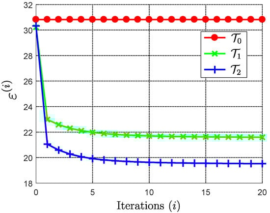
Here, for the case of optimal injections, we wish to numerically illustrate Theorem 10, i.e., that the error ${\epsilon }^{(i)}$ decreases if the number of iterations i increases.

For $i=0,1,\dots ,$ we denote

$${\displaystyle {\mathcal{T}}_p^{(i,i+1)}({\mathbf{v}}_0,{\mathbf{v}}_1^{(i+1)},\dots ,{\mathbf{v}}_p^{(i+1)})={\displaystyle \sum _{k=0}^p}{G}_k^{(i)}{H}_k^{(i)}{\mathbf{z}}_k({\mathbf{v}}_k^{(i+1)})}$$

and

$${\displaystyle {\mathcal{T}}_p^{(i+1,i)}({\mathbf{v}}_0,{\mathbf{v}}_1^{(i)},\dots ,{\mathbf{v}}_p^{(i)})={\displaystyle \sum _{k=0}^p}{G}_k^{(i+1)}{H}_k^{(i+1)}{\mathbf{z}}_k({\mathbf{v}}_k^{(i)}).}$$

According to the procedure described in Section 4, for each i-th iteration where $i=0,1,\dots$, the proposed method is represented by either

$${\mathcal{T}}_p^{(i,i+1)}({\mathbf{v}}_0,{\mathbf{v}}_1^{(i+1)},\dots ,{\mathbf{v}}_p^{(i+1)})$$

or

$${\mathcal{T}}_p^{(i+1,i)}({\mathbf{v}}_0,{\mathbf{v}}_1^{(i)},\dots ,{\mathbf{v}}_p^{(i)}).$$

To simplify the notation, both ${\mathcal{T}}_p^{(i,i+1)}({\mathbf{v}}_0,$ ${\mathbf{v}}_1^{(i+1)},$ $\dots ,{\mathbf{v}}_p^{(i+1)})$ and ${\mathcal{T}}_p^{(i+1,i)}({\mathbf{v}}_0,$ ${\mathbf{v}}_1^{(i)},\dots ,{\mathbf{v}}_p^{(i)})$ are denoted by ${\mathcal{T}}_p^{(i)}({\mathbf{v}}^{(i)})$.

We assume that $\mathbf{x}\in L^2(\Omega ,{\mathbb{R}}^m)$ and $\mathbf{y}\in L^2(\Omega ,{\mathbb{R}}^m)$ are uniformly and normally distributed random vectors, respectively. Initial injections ${\mathbf{v}}_1^{(0)}\in L^2(\Omega ,{\mathbb{R}}^{q_1}),\dots ,{\mathbf{v}}_p^{(0)}\in L^2(\Omega ,{\mathbb{R}}^{q_p})$ are here chosen as uniformly distributed random vectors. It is assumed that covariance matrices $E_{x{v}_j}$, $E_{v_i{v}_j}$, for $i,j=0,1,2$, are given by $E_{x{v}_j}={\displaystyle \frac{1}{s}}X{V}_j^{T}and{E}_{v_i{v}_j}={\displaystyle \frac{1}{s}}{V}_i{V}_j^T$ where $X\in {\mathbb{R}}^{m\times s}$ and $V_j\in {\mathbb{R}}^{q_j\times s}$ are samples of $\mathbf{x}$ and ${\mathbf{v}}_j$, respectively, for $j=0,1,2$.

We choose $m=400$ and $r_0=200$. In Table 3, values of error ${\epsilon }^{(i)}$ associated with operators ${\mathcal{T}}_0^{(i)}({\mathbf{v}}^{(i)})$, ${\mathcal{T}}_1^{(i)}({\mathbf{v}}^{(i)})$ and ${\mathcal{T}}_2^{(i)}({\mathbf{v}}^{(i)})$, for $i=14$ are represented.

Table 3. Numerical characterizations of approximating operators ${\mathcal{T}}_0^{(i)}({\mathbf{v}}^{(i)})$, ${\mathcal{T}}_1^{(i)}({\mathbf{v}}^{(i)})$ and ${\mathcal{T}}_2^{(i)}({\mathbf{v}}^{(i)})$.

${\mathcal{T}}_{\mathit{p}}^{(\mathit{i})}({\mathit{v}}^{(\mathit{i})})$	${\mathit{q}}_0$	${\mathit{q}}_1$	${\mathit{q}}_2$	${\mathit{r}}_0$	${\mathit{r}}_1$	${\mathit{r}}_2$	i	${\mathit{\epsilon }}^{(\mathit{i})}$
${\mathcal{T}}_0^{(i)}({\mathbf{v}}^{(i)})$	400	N/A	N/A	200	N/A	N/A	N/A	30.9
${\mathcal{T}}_1^{(i)}({\mathbf{v}}^{(i)})$	400	400	400	100	100	N/A	14	21.8
${\mathcal{T}}_2^{(i)}({\mathbf{v}}^{(i)})$	400	400	400	67	67	66	14	18.9

In Figure 3, diagrams of the errors are represented. It follows from Table 3 and Figure 3 that the error decreases if the number of iterations i increases. In particular, the error remains the same after $i=14$.

Figure 3. Example 2: Diagrams of the errors associated with ${\mathcal{T}}_0:={\mathcal{T}}_0^{(i)}({\mathbf{v}}^{(i)})$, ${\mathcal{T}}_1:={\mathcal{T}}_1^{(i)}({\mathbf{v}}^{(i)})$ and ${\mathcal{T}}_2:={\mathcal{T}}_2^{(i)}({\mathbf{v}}^{(i)})$.

Similar to what is explained in Example 1, the proposed method is more effective because the increase in the number of parameters to optimize in the operator $\mathcal{T}$ leads to the reduction in the error, as stated in Theorem 10.

References

- Amat, S.; Busquier, S.; Negra, M. Adaptive Approximation of Nonlinear Operators. Numer. Funct. Anal. Optim. 2004, 25, 397–405. [Google Scholar] [CrossRef]
- Bruno, V.I. An approximate Weierstrass theorem in topological vector space. J. Approx. Theory 1984, 42, 1–3. [Google Scholar] [CrossRef]
- Chen, T.; Chen, H. Universal approximation to nonlinear operators by neural networks with arbitrary activation functions and its application to dynamical systems. IEEE Trans. Neural Netw. 1995, 6, 911–917. [Google Scholar] [CrossRef]
- Dingle, K.; Camargo, C.Q.; Louis, A.A. Input–output maps are strongly biased towards simple outputs. Nat. Commun. 2018, 9, 761. [Google Scholar] [CrossRef]
- Gallman, P.G.; Narendra, K. Representations of nonlinear systems via the Stone-Weierstrass theorem. Automatica 1976, 12, 619–622. [Google Scholar] [CrossRef]
- Howlett, P.G.; Torokhti, A.P.; Pearce, C.E.M. A Philosophy for the Modelling of Realistic Non-linear Systems. Proc. Am. Math. Soc. 2003, 131, 353–363. [Google Scholar] [CrossRef]
- Istrăţescu, V.I. A Weierstrass theorem for real Banach spaces. J. Approx. Theory 1977, 19, 118–122. [Google Scholar] [CrossRef]
- Prenter, P.M. A Weierstrass Theorem for Real, Separable Hilbert Spaces. J. Approx. Theory 1970, 4, 341–357. [Google Scholar] [CrossRef]
- Prolla, J.B.; Machado, S. Weierstrass-Stone theorems for set-valued mappings. J. Approx. Theory 1982, 36, 1–15. [Google Scholar] [CrossRef]
- Rao, N.V. Stone-Weierstrass theorem revisited. Am. Math. Mon. 2005, 112, 726–729. [Google Scholar] [CrossRef]
- Sandberg, I.W. Notes on uniform approximation of time–varying systems on finite time intervals. IEEE Trans. Circuits Syst. I Fundam. Theory Appl. 1998, 45, 863–864. [Google Scholar] [CrossRef]
- Sandberg, I.W. Time delay polynomial networks and quality of approximation. IEEE Trans. Circuits Syst. I Fundam. Theory Appl. 2000, 47, 40–49. [Google Scholar] [CrossRef]
- Sandberg, I.W. R+ Fading Memory and Extensions of Input-Output Maps. IEEE Trans. Circuits Syst. I Fundam. Theory Appl. 2002, 49, 1586–1591. [Google Scholar] [CrossRef]
- Timofte, V. Stone-Weierstrass theorem revisited. J. Approx. Theory 2005, 536, 45–59. [Google Scholar] [CrossRef][Green Version]
- Piotrowski, T.; Cavalcante, R.; Yamada, I. Stochastic MV-PURE Estimator-Robust Reduced-Rank Estimator for Stochastic Linear Model. IEEE Trans. Signal Process. 2009, 57, 1293–1303. [Google Scholar] [CrossRef]
- Hua, Y.; Nikpour, M.; Stoica, P. Optimal reduced-rank estimation and filtering. IEEE Trans. Signal Process. 2001, 49, 457–469. [Google Scholar]
- Zhu, X.L.; Zhang, X.D.; Ding, Z.Z.; Jia, Y. Adaptive nonlinear PCA algorithms for blind source separation without prewhitening. IEEE Trans. Circuits Syst. I Regul. Pap. 2006, 53, 745–753. [Google Scholar]
- Wang, Q.; Jing, Y. New rank detection methods for retuced-rank MIMO systems. EURASIP J. Wirel. Comm. Netw. 2015, 2015, 1–16. [Google Scholar] [CrossRef]
- Bai, L.; Dou, S.; Xiao, Z.; Choi, J. Doubly iterative multiple-input-multiple-output-bit-interleaved coded modulation receiver with joint channel estimation and randomised sampling detection. IET Signal Process. 2016, 10, 335–341. [Google Scholar] [CrossRef]
- Brillinger, D.R. Time Series: Data Analysis and Theory; SIAM: San Francisco, CA, USA, 2001. [Google Scholar]
- Jolliffe, I. Principal Component Analysis, 2nd ed.; Springer: New York, NY, USA, 2002. [Google Scholar]
- Bühlmann, P.; van de Geer, S. Statistics for High-Dimensional Data; Springer: New York, NY, USA, 2011. [Google Scholar]
- She, Y.; Li, S.; Wu, D. Robust Orthogonal Complement Principal Component Analysis. J. Am. Stat. Assoc. 2016, 111, 763–771. [Google Scholar] [CrossRef]
- Torokhti, A.; Friedland, S. Towards theory of generic Principal Component Analysis. J. Multivar. Anal. 2009, 100, 661–669. [Google Scholar] [CrossRef]
- Saghri, J.A.; Schroeder, S.; Tescher, A.G. Adaptive two-stage Karhunen-Loeve-transform scheme for spectral decorrelation in hyperspectral bandwidth compression. Opt. Eng. 2010, 49, 057001. [Google Scholar] [CrossRef]
- Kmuntchav, R.; Kountcheva, R. Hierarchical Adaptive KL-Based Transform: Algorithms and Applications. In Computer Vision in Control Systems-1; Favorskaya, M.N., Jain, L.C., Eds.; Springer: Cham, Switzerland, 2015; Volume 73, pp. 91–136. [Google Scholar]
- de Moura, E.P.; de Abreu Melo Junior, F.; Damasceno, F.; Figueiredo, L.; de Andrade, C.; de Almeida, M. Classification of imbalance levels in a scaled wind turbine through detrended fluctuation analysis of vibration signals. Renew. Energy 2016, 96 Pt A, 993–1002. [Google Scholar] [CrossRef]
- Azimia, R.; Ghayekhlooa, M.; Ghofranib, M.; Sajedic, H. A novel clustering algorithm based on data transformation approaches. Expert Syst. Appl. 2017, 76, 59–70. [Google Scholar] [CrossRef]
- Burge, M.J.; Burger, W. Digital Image Processing—An Algorithmic Introduction Using Java; Springer: London, UK, 2006. [Google Scholar]
- Phophalia, A.; Rajwade, A.; Mitra, S.K. Rough set based image denoising for brain MR images. Signal Process. 2014, 103, 24–35. [Google Scholar] [CrossRef]
- Chenn, S.; Billings, S.A.; Grant, P. Non-linear system identification using neural networks. Int. J. Control 1990, 51, 1191–1214. [Google Scholar] [CrossRef]
- Chenn, S.; Billings, S.A. Neural networks for nonlinear dynamic system modelling and identification. Int. J. Control 1992, 56, 319–346. [Google Scholar] [CrossRef]
- Fomin, V.N.; Ruzhansky, M.V. Abstract Optimal Linear Filtering. SIAM J. Control Optim. 2000, 38, 1334–1352. [Google Scholar] [CrossRef]
- Temlyakov, V.N. Nonlinear Methods of Approximation. Found. Comput. Math. 2003, 3, 33–107. [Google Scholar] [CrossRef]
- Torokhti, A.; Howlett, P. Best approximation of identity mapping: The case of variable memory. J. Approx. Theory 2006, 143, 111–123. [Google Scholar] [CrossRef]
- Liu, W.; Zhang, H.; Yu, K.; Tan, X. Optimal linear filtering for networked systems with communication constraints, fading measurements, and multiplicative noises. Int. J. Adapt. Control Signal Process. 2016. [Google Scholar] [CrossRef]
- Aminzare, Z.; Sontag, E.D. Synchronization of Diffusively-Connected Nonlinear Systems: Results Based on Contractions with Respect to General Norms. IEEE Trans. Netw. Sci. Eng. 2014, 1, 91–106. [Google Scholar] [CrossRef]
- Schneider, M.K.; Willsky, A.S. A Krylov Subspace Method for Covariance Approximation and Simulation of Random Processes and Fields. Multidimens. Syst. Signal Process. 2003, 14, 295–318. [Google Scholar] [CrossRef]
- Chenn, S.; Billings, S.A. Representations of non-linear systems: The NARMAX model. Int. J. Control 1989, 49, 1013–1032. [Google Scholar] [CrossRef]
- Piroddi, L.; Spinelli, W. An identification algorithm for polynomial NARX models based on simulation error minimization. Int. J. Control 2003, 76, 1767–1781. [Google Scholar] [CrossRef]
- Alter, O.; Golub, G.H. Singular value decomposition of genome-scale mRNA lengths distribution reveals asymmetry in RNA gel electrophoresis band broadening. Process. Natl. Acad. Sci. USA 2006, 103, 11828–11833. [Google Scholar] [CrossRef]
- Gianfelici, F.; Turchetti, C.; Crippa, P. A non-probabilistic recognizer of stochastic signals based on KLT. Signal Process. 2009, 89, 422–437. [Google Scholar] [CrossRef]
- Formaggia, L.; Quarteroni, A.; Veneziani, A. (Eds.) Cardiovascular Mathematics—Modeling and Simulation of the Circulatory System; Springer: Milano, Italy, 2009; Volume 1. [Google Scholar]
- Ambrosi, D.; Quarteroni, A.; Rozza, G. (Eds.) Modelling of Physiological Flows; Springer: Milano, Italy, 2011; Volume V. [Google Scholar]
- Piotrowski, T.; Yamada, I. Performance of the stochastic MV-PURE estimator in highly noisy settings. J. Frankl. Insitute 2014, 351, 3339–3350. [Google Scholar] [CrossRef]
- Poor, H.V. An Introduction to Signal Processing and Estimation, 2nd ed.; Springer: New York, NY, USA, 2001. [Google Scholar]
- Torokhti, A.; Soto-Quiros, P. Optimal modeling of nonlinear systems: Method of variable injections. Proyecciones 2024, 43, 189–224. [Google Scholar] [CrossRef]
- Yang, S.; Xing, T.; Ke, C.; Liang, J.; Ke, X. Effect of wavefront distortion on the performance of coherent detection systems: Theoretical analysis and experimental research. Photonics 2023, 10, 493. [Google Scholar] [CrossRef]
- Stanković, L.; Brajović, M.; Stanković, I.; Lerga, J.; Daković, M. RANSAC-based signal denoising using compressive sensing. Circuits Syst. Signal Process. 2021, 40, 3907–3928. [Google Scholar] [CrossRef]
- Wang, Y.; Cheng, K.; Zhao, S.; Xu, E. Human ear image recognition method using PCA and Fisherface complementary double feature extraction. J. Artif. Intell. Technol. 2023, 3, 18–24. [Google Scholar] [CrossRef]
- Al-Saffar, N.F.H.; Al-Saiq, I.R. Symmetric text encryption scheme based Karhunen Loeve transform. J. Discret. Math. Sci. Cryptogr. 2022, 25, 2773–2781. [Google Scholar] [CrossRef]
- Soto-Quiros, P.; Torokhti, A. Fast random vector transforms in terms of pseudo-inverse within the Wiener filtering paradigm. J. Comput. Appl. Math. 2024, 448, 115927. [Google Scholar] [CrossRef]
- Howlett, P.; Torokhti, A. Optimal approximation of a large matrix by a sum of projected linear mappings on prescribed subspaces. Electron. J. Linear Algebra 2024, 40, 585–605. [Google Scholar] [CrossRef]
- Torokhti, A.; Howlett, P. Optimal estimation of distributed highly noisy signals within KLT-Wiener archetype. Digit. Signal Process. 2023, 143, 104225. [Google Scholar] [CrossRef]
- Howlett, P.; Torokhti, A. An optimal linear filter for estimation of random functions in Hilbert space. ANZIAM J. 2020, 62, 274–301. [Google Scholar] [CrossRef]
- Ledoit, O.; Wolf, M. A well-conditioned estimator for large-dimensional covariance matrices. J. Multivar. Anal. 2004, 88, 365–411. [Google Scholar] [CrossRef]
- Ledoit, O.; Wolf, M. Nonlinear shrinkage estimation of large-dimensional covariance matrices. Ann. Stat. 2012, 40, 1024–1060. [Google Scholar] [CrossRef]
- Adamczak, R.; Litvak, A.E.; Pajor, A.; Tomczak-Jaegermann, N. Quantitative estimates of the convergence of the empirical covariance matrix in log-concave ensembles. J. Am. Math. Soc. 2009, 2, 535–561. [Google Scholar] [CrossRef]
- Vershynin, R. How Close is the Sample Covariance Matrix to the Actual Covariance Matrix? J. Theor. Probab. 2012, 25, 655–686. [Google Scholar] [CrossRef]
- Won, J.-H.; Lim, J.; Kim, S.-J.; Rajaratnam, B. Condition-number-regularized covariance estimation. J. R. Stat. Soc. Ser. B 2013, 75, 427–450. [Google Scholar] [CrossRef] [PubMed]
- Yang, R.; Berger, J.O. Estimation of a covariance matrix using the reference prior. Ann. Statist. 1994, 22, 1195–1211. [Google Scholar] [CrossRef]
- Ben-Israel, A.; Greville, T.N.E. Generalized Inverses: Theory and Applications, 2nd ed.; Springer: New York, NY, USA, 2003. [Google Scholar]
- Hotelling, H. Analysis of a Complex of Statistical Variables into Principal Components. J. Educ. Psychol. 1933, 6, 417–441 and 498–520. [Google Scholar] [CrossRef]
- Karhunen, K. Über Lineare Methoden in der Wahrscheinlichkeitsrechnung. Ann. Acad. Sci. Fenn. Ser. A. I. Math.-Phys. 1947, 1, 1–79. [Google Scholar]
- Loève, M. Fonctions aléatoires de second ordre. In Processus Stochastiques et Mouvement Brownien; Lévy, P., Ed.; Hermann: Paris, France, 1948. [Google Scholar]
- Scharf, L. The SVD and reduced rank signal processing. Signal Process. 1991, 25, 113–133. [Google Scholar] [CrossRef]
- Hua, Y.; Liu, W. Generalized Karhunen-Loeve transform. IEEE Signal Process. Lett. 1998, 5, 141–142. [Google Scholar]
- Torokhti, A.; Soto-Quiros, P. Generalized Brillinger-Like Transforms. IEEE Signal Process. Lett. 2016, 23, 843–847. [Google Scholar] [CrossRef]
- Torokhti, A.; Miklavcic, S. Data compression under constraints of causality and variable finite memory. Signal Process. 2010, 90, 2822–2834. [Google Scholar] [CrossRef]
- Lathauwer, L.D.; Moor, B.D.; Vandewalle, J. On the Best Rank-1 and Rank-(R1,R2, …, RN) Approximation of Higher-Order Tensors. SIAM J. Matrix Anal. Appl. 2006, 21, 1324–1342. [Google Scholar] [CrossRef]
- Grasedyck, L.; Kressner, D.; Tobler, C. A literature survey of low-rank tensor approximation techniques. GAMM-Mitteilungen 2013, 36, 53–78. [Google Scholar] [CrossRef]
- Friedland, S.; Tammali, V. Low-Rank Approximation of Tensors. In Numerical Algebra, Matrix Theory, Differential-Algebraic Equations and Control Theory; Benner, P., Bollhöfer, M., Kressner, D., Mehl, C., Stykel, T., Eds.; Springer: Cham, Switzerland, 2015; pp. 377–411. [Google Scholar]
- Billings, S.A. Nonlinear System Identification-Narmax Methods in the Time, Frequency, and Spatio-Temporal Domains; John Wiley and Sons, Ltd.: Hoboken, NJ, USA, 2013. [Google Scholar]
- Schoukens, M.; Tiels, K. Identification of Block-oriented Nonlinear Systems Starting from Linear Approximations: A Survey. Automatica 2017, 85, 272–292. [Google Scholar] [CrossRef]
- Chen, B.; He, S.; Li, Z.; Zhang, S. Maximum Block Improvement and Polynomial Optimization. SIAM J. Optim. 2012, 22, 87–107. [Google Scholar] [CrossRef]
- Abed-Meraim, K.; Qui, W.; Hua, Y. Blind system identification. Proc. IEEE 1997, 85, 1310–1322. [Google Scholar] [CrossRef]
- Hua, Y. Blind methods of system identification. Circuits Syst. Signal Process. 2002, 21, 91–108. [Google Scholar] [CrossRef]
- Shi, X. Mathematical Description of Blind Signal Processing. In Blind Signal Processing: Theory and Practice; Springer: Berlin/Heidelberg, Germany, 2011; pp. 27–59. [Google Scholar]
- Torokhti, A.; Howlett, P. Optimal Fixed Rank Transform of the Second Degree. IEEE Trans. Circuits Syst. II Analog. Digit. Signal Process. 2001, 48, 309–315. [Google Scholar] [CrossRef]
- Torokhti, A.; Howlett, P. Computational Methods for Modelling of Nonlinear Systems; Elsevier: Amsterdam, The Netherlands, 2007. [Google Scholar]
- Friedland, S.; Torokhti, A. Generalized Rank-Constrained Matrix Approximations. SIAM J. Matrix Anal. Appl. 2007, 29, 656–659. [Google Scholar] [CrossRef][Green Version]
- Liu, X.; Li, W.; Wang, H. Rank constrained matrix best approximation problem with respect to (skew) Hermitian matrices. J. Comput. Appl. Math. 2017, 319, 77–86. [Google Scholar] [CrossRef]
- Boutsidis, C.; Woodruff, D.P. Optimal CUR Matrix Decompositions. SIAM J. Comput. 2017, 46, 543–589. [Google Scholar] [CrossRef]
- Wang, H. Rank constrained matrix best approximation problem. Appl. Math. Lett. 2015, 50, 98–104. [Google Scholar] [CrossRef]
- Golub, G.; Loan, C.F.V. Matrix Computations; Jons Hopkins University Press: Baltimore, MD, USA, 1996. [Google Scholar]
- Kanwal, R. Linear Integral Equations; Birkhäuser Boston: Boston, MA, USA, 1996. [Google Scholar]
Disclaimer/Publisher’s Note: The statements, opinions and data contained in all publications are solely those of the individual author(s) and contributor(s) and not of MDPI and/or the editor(s). MDPI and/or the editor(s) disclaim responsibility for any injury to people or property resulting from any ideas, methods, instructions or products referred to in the content. |
© 2025 by the authors. Licensee MDPI, Basel, Switzerland. This article is an open access article distributed under the terms and conditions of the Creative Commons Attribution (CC BY) license (https://creativecommons.org/licenses/by/4.0/).