A Novel Mutual Information and Partial Least Squares Approach for Quality-Related and Quality-Unrelated Fault Detection

Abstract

Partial least squares (PLS) and linear regression methods are widely utilized for quality-related fault detection in industrial processes. Standard PLS decomposes the process variables into principal and residual parts. However, as the principal part still contains many components unrelated to quality, if these components were not removed it could cause many false alarms. Besides, although these components do not affect product quality, they have a great impact on process safety and information about other faults. Removing and discarding these components will lead to a reduction in the detection rate of faults, unrelated to quality. To overcome the drawbacks of Standard PLS, a novel method, MI-PLS (mutual information PLS), is proposed in this paper. The proposed MI-PLS algorithm utilizes mutual information to divide the process variables into selected and residual components, and then uses singular value decomposition (SVD) to further decompose the selected part into quality-related and quality-unrelated components, subsequently constructing quality-related monitoring statistics. To ensure that there is no information loss and that the proposed MI-PLS can be used in quality-related and quality-unrelated fault detection, a principal component analysis (PCA) model is performed on the residual component to obtain its score matrix, which is combined with the quality-unrelated part to obtain the total quality-unrelated monitoring statistics. Finally, the proposed method is applied on a numerical example and Tennessee Eastman process. The proposed MI-PLS has a lower computational load and more robust performance compared with T-PLS and PCR.

1. Introduction

Process quality monitoring methods can be divided into two types: Direct monitoring and processed monitoring. Direct monitoring, the traditionally used quality monitoring method, is based on the different characteristics of quality variables, chooses a suitable method to model the quality variables directly, and monitors the changes in the quality variables. Processed monitoring methods use quality variables to supervise and model process variables, use orthogonal decomposition to extract quality-related features in the process variables and project the process variable space into quality-related and quality-unrelated feature spaces. If the number of quality variables is not large, univariate statistical graph methods can be directly applied for monitoring, such as Shewhart plots, cumulative sum (CUSUM) plots, and exponentially weighted moving average (EWMA) plots. [1]. This has good detection performance for short-term and severe fault conditions. When the number of quality variables is large, multivariate statistical analysis methods can be applied. Among these methods, principal component analysis (PCA) is a relatively basic process monitoring method and has been extensively used in research [2,3,4,5].

In actual production operations, most quality variables are difficult to obtain by direct online measurement. For example, in the petrochemical production process, the product concentration or purity requires further offline analysis and inspection with the help of analytical testing instruments. If the energy consumption of the process operation is considered, a variety of performance indicators need to be integrated before the calculation can be performed. The online measurement and application of these quality variables are often time-consuming and involve certain delays. Therefore, when implementing a direct quality monitoring method, the steps of quality prediction need to be completed before modeling and monitoring are performed.

The key to direct quality monitoring methods is quality prediction and obtaining accurate prediction results is the core of subsequent quality monitoring steps. Extensive research has focused on improving modeling accuracy, reducing prediction errors, and ensuring prediction accuracy for online applications. Based on previous research, Chen et al. [6] divided the prediction process into three main aspects: feature (variable) selection, predictive modeling, and parameter optimization. Therefore, we can start from these three aspects and study how to improve the prediction accuracy.

First, feature (variable) selection attempts to use only the most relevant quality variables of the process variable, eliminating weakly related and unrelated variables. Such dimension reduction helps to reduce the computational complexity of the process, while improving the prediction accuracy and modeling efficiency. Second, with regard to predictive modeling, the appropriate forecasting model is mainly selected based on different forecasting requirements or different data characteristics, depending on the production conditions [6]. For example, short- and long-term prediction models can be used according to the prediction duration, single- and multiple-output models can be used according to the number of quality variables, data-driven models and data-mechanism hybrids model can be used depending on whether or not mechanism knowledge is combined, and single and integrated models can be used according to the distribution of data [7,8] Finally, in terms of parameter optimization, the basic idea is to use a regression model built based on different objective functions to analyze the critical parameters that should be optimized (regularization parameters, the number of hidden neurons in the neural network and the corresponding weight values; Kernel function parameters in the kernel method, etc.), which are mainly divided into offline and online optimization. Offline optimization aims to minimize prediction error and variance or optimize the probability density function of the prediction error, and uses gradient descent, conjugate gradient, and intelligent optimization methods, among others [9], to obtain the optimal solution. Online optimization methods are based on a comparison between the predicted value at each step and the real value, and simulation models in the Simulink environment [10,11,12]. The extraction method is used to predict the error compensation to make online corrections to the next predicted value and continuously updates the model parameters to achieve a rolling optimization.

After obtaining accurate quality prediction results, modeling and direct monitoring can be carried out. The direct quality monitoring method intuitively reflects the change in the quality variable and has a good performance for the quality variable. The traditional PCA method only models and monitors variables. It belongs to an unsupervised learning method and cannot reflect the relationship between process variables and quality variables [13,14]. By contrast, the partial least squares (PLS) method supervises quality variables, linearly decomposing the process variable to obtain a regression model that can extract the correlation between the process variable and the quality variable [15]. It is often used for quality prediction and quality monitoring. Based on the improved PLS algorithm, Yin et al. [16] assumed that the industrial process can be described by a general linear time-invariant system, and established a soft measurement strategy in the framework of a diagnostic observer, and used generated residual signals for monitoring. Ding et al. [17] extended the method in [16] to a dynamic form, using the left coprime factorization method, combined with the above-mentioned soft measurement and residual monitoring framework, to achieve the quality prediction of dynamic processes. Both methods in [16] and [17] have been successfully applied in the process of the hot strip rolling industry, which has improved quality prediction accuracy and quality monitoring performance. However, both are based on linear conditions, and therefore are only applicable to linear processes.

Focusing on the problem of quality monitoring of non-linear processes, Ju et al. [18] combined wavelet variation and the kernel PLS (KPLS) method to propose a multi-scale KPLS algorithm. They established a wastewater treatment process key performance indicator—the COD concentration in the effluent—and monitored its change in real time. The method introduced in [18] is suitable for steady-state processes. When the actual process has time-varying conditions, its monitoring performance decreases. In order to solve the problem of quality prediction and monitoring of nonlinear multi-period intermittent processes, Yu et al. [19] proposed a multi-directional Gaussian mixed model for period division and identification. In each period, multiple local KPLS regression models are built to perform quality prediction. The Bayesian inference strategy was used to adaptively select a suitable local model for online prediction based on the maximum posterior probability. This method combines the variable selection and the predictive modeling optimization methods described above. The PLS method uses data for modeling and can effectively solve the problem of variable collinearity, and is suitable for multi-output predictions and quality monitoring of multi-variable processes [20,21]. PLS has been studied and applied in quality monitoring and many other fields [22,23].

In this paper, we propose a novel mutual information partial least squares (MI-PLS) approach for quality-related and quality-unrelated monitoring. The proposed method considers quality-related and quality-unrelated faults to ensure there are no false alarms and no missed alarms. We then apply it to a numerical example and Tennessee Eastman (TE) process to verify its effectiveness.

2. Related Work

The principal component analysis (PCA) algorithm models process variables and can be regarded as an unsupervised learning algorithm, ignoring quality variables and their relationship with process variables. PLS utilizes quality variables to guide the modeling of process variables, and the latent variables obtained by decomposing the process variables can reflect the quality-related parts. Therefore, PLS is also called projection to latent structure (PLS) [16]. Here, we assume that the normalized process variable can be expressed as $X$, the quality variable as y, and that $n$ is the number of samples, and $p$ and $q$ are the number of process variables and quality variables, respectively. PLS linearly decomposes $X$ and $Y$ to obtain the following regression model

$$\{\begin{array}{l}X=T{P}^{\mathrm{T}}+E\\ Y=U{Q}^{\mathrm{T}}+F\end{array}$$

(1)

where $T=\left[t_1,t_2,\cdots t_d\right]\in R^{n\times d}$ and $U=\left[u_1,u_2,\cdots ,u_d\right]\in R^{n\times d}$ denotes the score matrices of the input $X$ and the output $Y$, $P$ and $Q$ represents the loading matrices of the input, $X$, and the output $Y$, $E$ and $F$ denotes the residual parts; $t_i$ and $u_i$ are the $i$th latent variables extracted, and $d$ is the number of latent variables retained. In the process of applying PLS, the most commonly used method is nonlinear iterative partial least squares (NIPALS) [16], which follows the steps in Algorithm 1. During an iteration, the goal of PLS is to maximize the covariance of $t_i$ and $u_i$.

Algorithm 1. The Description of NIPALS Algorithm, Nonlinear Iterative Partial Least Squares (NIPALS) Algorithm Description

Let $i=1$, start. (1) Take any column in $Y$ and record as $u_i$. (2) Calculate the regression of each column in $X$ on $u_i$, and get the regression matrix as $w_i=X^T{u}_i/u_i^T{u}_i$. (3) Normalize $w_i$ and calculate the score vector for $X$ as $t_i=X{w}_i$. (4) Calculate the regression of each column in $Y$ on $t_i$, and get the load matrix of $Y$ as $q_i={Y^T{t}_i/t_i^{T}t}_i$. (5) Compute the new score vector for $Y$ as $u_i=Y{q}_i$. (6) If $u_i$ converges, go to step (7), otherwise return to step (2). (7) Calculate the load matrix of $X$ as $p_i=X^T{t}_i/t_i^T{t}_i$. (8) Calculate the residual matrices for $X$ and $Y$ as $E=X-t_i{p}_i^T$ and $F=Y-u_i{q}_i^T$, respectively. (9) Replace $E$ and $F$ with $X$ and $Y$, respectively, and let $i=i+1$ return to step (1); repeat the calculation until $d$ latent variables are extracted, that is, stop iteration at $i>d$.

In order to achieve process monitoring, similar to PCA, a $T_i^2$ monitoring statistic can be built in the score matrix $T$, as shown in the following equation

$$T_i^2=x_i^{\mathrm{T}}R{\left(\frac{T^{\mathrm{T}}T}{n-1}\right)}^{-1}{R}^T{x}_i$$

(2)

where $R$ is the projection matrix, which can be calculated by

$$R=W{\left(P^{\mathrm{T}}W\right)}^{-1}$$

(3)

The matrices in Equation (3) satisfy the following relationship: $P^{\mathrm{T}}R=R^{\mathrm{T}}P=W^{\mathrm{T}}W=I_d$, where $I_d$ represents the identity matrix with dimension $d$. Similarly, the KDE method can be used to estimate its control limit. During the online application, the value of the statistic corresponding with the new sample is calculated and compared with the control limit to determine whether the process is normal or not, and $T_i^2$ can reflect the changes related to $Y$ in $X$. By comparing the monitoring statistic and the control limit, it is possible to determine whether the fault condition occurring in $X$ affects the quality variable $Y$.

However, for standard PLS, the process variable $x$ is decomposed into a quality-related part $\widehat{\mathit{x}}$ and a quality-unrelated part $\tilde{\mathit{x}}$, but the quality-related part $\widehat{\mathit{x}}$ still contains some components unrelated to the output $Y$, so these components should be removed to avoid false alarms. Besides, in standard PLS, the variance in $X$ is extracted by maximizing the covariance between process variables (input) and quality variables (output), without necessarily being in descending order [24]. As a result, the residual component may consist of some variables responsible for predicting the output $Y$. Due to these drawbacks of standard PLS, a novel method is proposed in this paper, namely, MI-PLS, which takes these problems into consideration and further decomposes $\widehat{\mathit{x}}$ but does not “discard” the residual of $\tilde{\mathit{x}}$, to ensure that no information is lost from either the quality-related or quality-unrelated parts.

3. Quality-Related and Quality-Unrelated Fault Detection Based on MI-PLS

In this section, our novel PLS based on the mutual information quality variable selection method is presented. The proposed method is easy and effective for quality-related and quality-unrelated faults. MI-PLS is applied to a numerical example and compared with PCR and TPLS.

3.1. A Novel Quality Variables Selection Based on Mutual Information

Mutual information (MI) is an effective measure of information in probability theory and information theory, and is a quantitative representation of the statistical dependence between two sets of variables. It can be used to measure the amount of process variable information contained in quality variables, that is, the correlation between the two. It is, therefore, also a type of correlation coefficient. Over recent years, mutual information has been used widely in the field of process monitoring for variable selection and process decomposition. Mutual information can be defined as the degree of correlation between the product of the joint distribution and the marginal distribution. Correspondingly, the mathematical expression is

$$M{I}_{i,j}={\displaystyle {\iint }_{X_i,Y_j}p\left(X_i,Y_j\right)}\log \left(\frac{p\left(X_i,Y_j\right)}{p\left(X_i\right)p\left(Y_j\right)}\right)d{X}_{i}d{Y}_j$$

(4)

where $i=\left(1,2,\cdots ,p\right)$ and $j=\left(1,2,\cdots ,q\right)$. In addition, $p\left(X_i,Y_j\right)$ represents the joint probability density function of the process variable, $X_i$, and quality variable, $Y_j$, and $p\left(X_i\right)$ and $p\left(Y_i\right)$ represent the marginal probability density function of $X_i$ and $Y_j$, respectively. When calculating mutual information, information entropy is mainly used and Equation (4) can be rewritten as

$$M{I}_{i,j}=H\left(X_i\right)+H\left(Y_j\right)-H\left(X_i,Y_j\right)$$

(5)

where $H\left(X_i\right)$ and $H\left(Y_j\right)$ represent the marginal entropy of $X_i$ and $Y_j$, respectively, which can be calculated as follows

$$\{\begin{array}{c}H\left(X_i\right)=-{\displaystyle {\int }_{X_i}p\left(X_i\right)\log p\left(X_i\right)d{X}_i}\\ H\left(Y_j\right)=-{\displaystyle {\int }_{Y_j}p\left(Y_j\right)\log p\left(Y_j\right)d{Y}_j}\end{array}$$

(6)

where $H\left(X_i,Y_j\right)$ represents the joint entropy, which can be calculated as

$$H\left(X_i,Y_j\right)=-{\displaystyle {\iint }_{X_i,Y_j}p\left(X_i,Y_j\right)}\log \left(p\left(X_i,Y_j\right)\right)d{X}_{i}d{Y}_j$$

(7)

According to the given process variable and quality variable, the mutual information can be calculated and the correlation between the two can be quantitatively described. The mutual information matrix is constructed as follows

$$M_{MI}=\left[\begin{array}{cccc}M{I}_{1,1}& M{I}_{1,2}& \cdots & M{I}_{1,q}\\ M{I}_{2,1}& M{I}_{2,2}& \cdots & M{I}_{2,q}\\ ⋮& ⋮& \ddots & ⋮\\ M{I}_{p,1}& M{I}_{p,2}& \cdots & M{I}_{p,q}\end{array}\right]$$

(8)

Sum up each row to obtain the total mutual information value of each process variable for all quality variables to form a total mutual information vector

$$To{M}_{MI}={\left[\begin{array}{cccc}M{I}_1& M{I}_2& \cdots & M{I}_p\end{array}\right]}^{\mathrm{T}}$$

(9)

Finally, the variable selection strategy based on mutual information will be

$$M{I}_i\ge mean\left(To{M}_{MI}\right)$$

(10)

The total mutual information value is greater than the mean value. Its corresponding process variable is selected.

3.2. The Proposed MI-PLS

After all the process variables are assigned, the input matrix $X$ is divided into two parts: the quality-related part, $X_{sel}$, and quality-unrelated part, $X_{res}$

$$X=X_{sel}+X_{res}$$

(11)

According to the preliminary part of PLS above, the regression coefficient between the latent variable and the quality variable is

$$\mathit{Q}={\left({\mathit{T}}^{\mathrm{T}}\mathit{T}\right)}^{-1}{\mathit{T}}^{\mathrm{T}}\mathit{Y}\in {\mathit{R}}^{\mathrm{m}\times \mathrm{l}}$$

(12)

where $\mathit{Q}$ is the regression coefficient, $\mathit{T}$ is the score matrix, and $\mathit{Y}$ is the output. Then, we perform singular value decomposition (SVD) on $Q{Q}^{\mathrm{T}}$

$$Q{Q}^{\mathrm{T}}=\left[\begin{array}{cc}\widehat{\mathit{U}}& \tilde{\mathit{U}}\end{array}\right]\left[\begin{array}{cc}\Lambda & 0\\ 0& 0\end{array}\right]\left[\begin{array}{c}{\widehat{\mathit{U}}}^{\mathrm{T}}\\ {\widehat{\mathit{U}}}^{\mathrm{T}}\end{array}\right]$$

(13)

where $\widehat{\mathit{U}}\in R^{m\times l}$, $\tilde{\mathit{U}}\in R^{m\times \left(m-l\right)}$, $\Lambda \in R^{l\times l}$. The orthogonal projection matrices of quality-related and quality-unrelated parts $\widehat{\mathit{\Pi }}$ and $\tilde{\mathit{\Pi }}$ subsequently should then be constructed as follows

$$\widehat{\mathit{\Pi }}=\widehat{\mathit{U}}{\widehat{\mathit{U}}}^{\mathrm{T}}\in R^{m\times m}$$

(14)

$$\tilde{\mathit{\Pi }}=\tilde{\mathit{U}}{\tilde{\mathit{U}}}^{\mathrm{T}}\in R^{m\times m}$$

(15)

where $\widehat{\mathit{\Pi }}$ denotes the projection matrix of quality-related part, and $\tilde{\mathit{\Pi }}$ is the projection matrix of the quality-unrelated part.

By projecting the input variable $X$ onto $\widehat{\mathit{\Pi }}$ and $\tilde{\mathit{\Pi }}$, two orthogonal subspaces, $\widehat{\mathit{X}}$ and $\tilde{\mathit{X}}$, are obtained by

$$\widehat{\mathit{X}}=\mathit{X}\widehat{\mathit{\Pi }}\in R^{N\times m}$$

(16)

$$\tilde{\mathit{X}}=\mathit{X}\tilde{\mathit{\Pi }}\in R^{N\times m}$$

(17)

where $\widehat{\mathit{X}}$ represents the quality-related subspace and $\tilde{\mathit{X}}$ represents the quality-unrelated subspace.

In the online monitoring, a new sample, $x$, can be divided into $\widehat{\mathit{x}}\in R^{l\times 1}$ and $\tilde{\mathit{x}}\in R^{\left(m-l\right)\times 1}$. We then take into consideration the quadratic forms of the new $\widehat{\mathit{x}}$ and $\tilde{\mathit{x}}$

$${\widehat{\mathit{x}}}^{\mathrm{T}}\widehat{\mathit{x}}=x^{\mathrm{T}}\widehat{\mathit{U}}{\widehat{\mathit{U}}}^T\widehat{\mathit{U}}{\widehat{\mathit{U}}}^{\mathrm{T}}x=t_{\widehat{x}}^{\mathrm{T}}{t}_{\widehat{x}}$$

(18)

$${\tilde{\mathit{x}}}^{\mathrm{T}}\tilde{\mathit{x}}=x^{\mathrm{T}}\tilde{\mathit{U}}{\tilde{\mathit{U}}}^T\tilde{\mathit{U}}{\tilde{\mathit{U}}}^{\mathrm{T}}x=t_{\tilde{x}}^{\mathrm{T}}{t}_{\tilde{x}}$$

(19)

$$t_{\widehat{x}}={\widehat{\mathit{U}}}^{\mathrm{T}}x$$

(20)

$$t_{\tilde{x}}={\tilde{\mathit{U}}}^{\mathrm{T}}x$$

(21)

where $t_{\widehat{x}}$ and $t_{\tilde{x}}$ are appropriate applicant for the monitoring statistic $T^2$; $t_{\widehat{x}}$ is directly used for $T^2$ statistics to monitor the quality-related part, $t_{\tilde{x}}$ is combined with the score matrix of the residual part, and used for $T^2$ statistics to monitor the quality-unrelated part.

The monitoring statistic of quality-related part is built as follows

$$T_{re}^2=t_{\widehat{x}}^{\mathrm{T}}{\left(\frac{T_{re}^{\mathrm{T}}{T}_{re}}{N-1}\right)}^{-1}{t}_{\widehat{x}}=x^{\mathrm{T}}\widehat{\mathit{U}}\left(\frac{{\widehat{\mathit{U}}}^{\mathrm{T}}{X}^{\mathrm{T}}\mathit{X}\widehat{\mathit{U}}}{N-1}\right){\widehat{\mathit{U}}}^{\mathrm{T}}x$$

(22)

where $T_{re}^2$ is the monitoring statistics of the quality-related component.

Then, PCA is performed on the residual, $X_{res}$, to obtain the latent variable matrix, $T_{res}$.

Therefore, the total latent variable of unrelated part is constructed by

$$T_{t,un}=\left[\begin{array}{cc}{T}_{\tilde{x}}& T_{res}\end{array}\right]$$

(23)

The quality-unrelated monitoring statistic is built as follows

$$T_{un}^2=T_{t,un}^{\mathrm{T}}{\left(\frac{T_{t,un}^{\mathrm{T}}{T}_{t,un}}{N-1}\right)}^{-1}{T}_{t,un}$$

(24)

where $T_{un}^2$ is the monitoring statistics of quality-unrelated part.

Thresholds of the monitoring statistics can be determined by kernel density estimation (KDE) and the control limit is presented as $j_{re}$ and $j_{un}$ for the quality-related part and quality-unrelated parts, respectively. The monitoring logic is as follows:

• $T_{re}^2>j_{re}$ quality-related fault.
• $T_{re}^2<j_{re}$ no quality-related fault.
• $T_{un}^2>j_{un}$ quality-related or unrelated fault.
• $T_{un}^2<j_{un}$ no quality-unrelated fault.

Finally, the main steps of the proposed MI-PLS can be summarized as follows:

• Construct the offline process variable and quality variable matrices $X$ and $Y$;
• Apply the proposed MI-based filtering method on the process variable matrix, $X$, and quality variable matrix, $Y$, as summarized in Section 3.2. The filtered process variable matrix is denoted as $X_{MI}$. The loading and weight matrices are represented as $P$ and $W$, respectively;
• Calculate the regression coefficient $Q$ by performing standard PLS onto the filtered process data, $X_{MI}$, and quality data, $Y$, using the NIPALS in Algorithm 1;
• Perform SVD on $Q{Q}^{\mathrm{T}}$ to obtain $\widehat{\mathit{\Pi }}$ and $\tilde{\mathit{\Pi }}$ by (13);
• For each online test sample $x_t$, correct it by $x_t^{\mathrm{T}}=x_t^{\mathrm{T}}-x_t^{\mathrm{T}}W{\left(P^{T}W\right)}^{-1}{P}^{\mathrm{T}}$;
• Perform PCA on $X_{res}$ and combine $T_{res}$ with $T_{\widehat{x}}$;
• Calculate statistics $T_{re}^2$ and $T_{un}^2$ by (22) and (24), where $x$ is $x_t$ and $X$ is $X_{MI}$;
• Calculate thresholds $j_{re}$ and $j_{un}$ by kernel density estimation (KDE);
• Diagnosis logic:
  • $T_{re}^2>j_{re}$ quality-related fault has occurred;
  • $T_{re}^2<j_{re}$ no quality-related fault has occurred;
  • $T_{un}^2>j_{un}$ quality-related or unrelated fault has occurred;
  • $T_{un}^2<j_{un}$ no fault unrelated to quality has occurred.

The superiorities of the proposed MI-PLS algorithm can be summarized as follows:

• MI-PLS requires few model latent variables; therefore, MI-PLS has a low computational load;
• MI-PLS utilizes the MI-based filtering method to remove variables that are irrelevant to quality before applying PLS. After this, it decomposes the selected part into quality-related and quality-unrelated subspaces in the postprocessing process; therefore, MI-PLS is more robust than other traditional methods;
• MI-PLS does not discard the residual, $X_{res}$; it participates in modeling and combines with unrelated parts from $X_{sel}$ to ensure no information is lost.

The schematic diagram of the proposed fault detection method is shown in Figure 1.

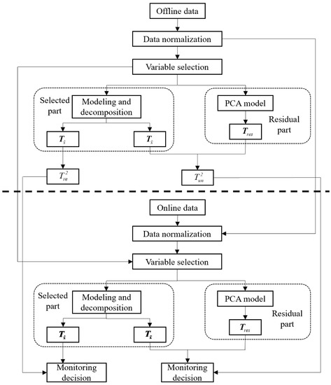
Figure 1. Schematic diagram of the proposed mutual information partial least squares (MI-PLS) approach.

4. Case Study

We used two case studies to test the proposed MI-PLS. The first is a numerical example and the second uses the TE process. In these experiments, PCR and T-PLS—two of the most commonly used methods in quality relevant and irrelevant fault detection—are used to provide a comparison among methods.

4.1. Numerical Example

We used this numerical example to test the effectiveness of the MI-PLS algorithm. Performance evaluation uses two indicators, namely, false alarm rate (FAR) and fault detection rate (FDR). FAR is the detection of faulty samples that are not related to quality, $Y$, whereas FDR indicates the detection of faulty samples relevant to quality $Y$. The FDR and FAR can be calculated as follows

$$FDR=\frac{N_d}{N_{fs}}\times 100\%$$

(25)

$$FAR=\frac{N_a}{N_{fs}}\times 100\%$$

(26)

where $N_{fs}$ represents the number of faulty samples, $N_a$ is the number of false alarms, and $N_d$ is the number of alarms.

From an industrial process perspective, a quality monitoring algorithm should be able to achieve the following

(1)

With regard to quality-irrelevant faults, a low false-alarm rate in quality relevant monitoring statistics, and high fault-detection rate in quality-irrelevant monitoring statistics;

(2)

For quality-relevant faults, a high fault-detection rate in quality relevant monitoring statistics, but no specific requirement in relation to quality-irrelevant monitoring statistics.

To determine whether the fault affects the quality variable $y$, a novel $Q$ statistic is proposed to directly monitor the output $y$ residual, which can be obtained as follows

$$Q_y={\Vert y-\widehat{\mathit{y}}\Vert }^2\sim g{\chi }_{\alpha ,h}^2$$

(27)

It is worth noting that $Q_y$ is only used for quality-related and quality-unrelated fault classification and not for process monitoring.

The numerical example is constructed as follows

$$\begin{array}{cc}{x}_1\sim N\left(1,{0.1}^2\right),& x_2\sim N\left(1,{0.1}^2\right)\end{array}$$

(28)

$$x_3=\sin \left(x_1\right)+m_1$$

(29)

$$x_4=x_1^2-3x_1+4+m_2$$

(30)

$$x_5=x_2^2+\cos \left(x_2^2\right)+1+m_3$$

(31)

$$y=x_3^2+x_3{x}_4+x_1+e$$

(32)

where $m_j\sim N\left(1,{0.001}^2\right)\left(j=1,2,3\right)$ and $e\sim N\left(1,{0.005}^2\right)$. When the fault occurs in $x_1$, the product quality, $y$, will be directly influenced. While the fault is added in $x_2$, it will not exert an effect on the product quality.

• Fault No.1: $x_2=x_2^{\ast }+x_f$, $x_f$ quality-irrelevant;
• Fault No.2: $x_2=x_2^{\ast }+\left(Nt-100\right)x_f$, $x_f$ quality-irrelevant;
• Fault No.3: $x_1=x_1^{\ast }+x_f$, $x_f$ quality-relevant;
• Fault No.4: $x_1=x_1^{\ast }+\left(Nt-100\right)x_f$, $x_f$ quality-relevant.

The selection of numbers can be based on the monitoring problem targeted by article. Here, the training sample $Nt$ is set as $Nt=200$. The test sample number is set as 200, in which the first 100 samples are normal data, and the other 100 samples are fault data. The models of MI-PLS and PCR were constructed from the training samples. In this work, we first select the key process variables. Figure 2 shows the mutual information between input variables and the output (quality) variable. Therefore, the first, third, and fourth process variables were chosen as the key process variables, as shown in Figure 2. Fault 1 was selected as quality-unrelated and Fault 3 as quality-related; they were chosen to demonstrate the performance of MI-PLS, T-PLS, and PCR.

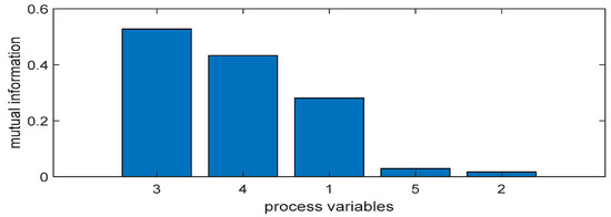
Figure 2. Mutual information between the quality variable and process variables.

• Case study on Fault 1: The fault $x_f$ is added to $x_2$

  $$x_2=x_2^{\ast }+x_f$$

  (33)

As shown in Figure 3, when Fault 1 occurred, the output $y$ was not affected; the changing trend of the quality variable in this state was unchanged, meaning Fault 1 was not related to quality.

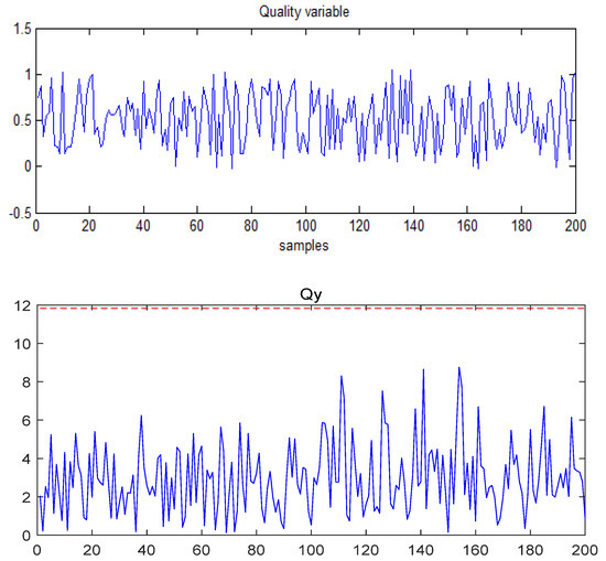
Figure 3. The quality variable $y$ and the $Q_y$ statistic for Fault 1.

Figure 4, Figure 5 and Figure 6 show the detection results of T-PLS, PCR, and the proposed MI-PLS, respectively. As shown in Figure 4, the $T_{un}^2$ part exceeded the control limit, which means that the quality-unrelated fault was successfully detected. However, $T_{re}^2$ exceeded the control limit as well, while in this case the fluctuations and changes in process variables should be regarded as normal disturbances or normal adjustments and responses of the process itself to external disturbances. The expectation for false alarms should be reduced, and there is no need to issue an alarm for such a fault.

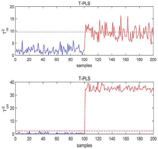
Figure 4. The monitoring results of T-PLS under Fault 1 conditions.

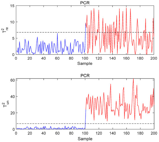
Figure 5. The monitoring results of PCR under Fault 1 conditions.

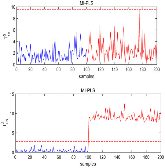
Figure 6. The monitoring results of MI-PLS under Fault 1 conditions.

The same situation can be observed in Figure 5. When the quality-unrelated fault occurs, the quality-related monitoring statistic gives an alarm because the FAR in T-PLS and PCR is so high, meaning that these methods cannot distinguish whether $y$ is affected or not under this fault. Therefore, T-PLS and PCR do not provide correct results, forcing the process into unnecessary stops and reconditioning.

In Figure 6, $T_{un}^2$ exceeds the control limit, but the quality-related part $T_{re}^2$ does not; this is the best result, as unnecessary alarms are avoided. Compared with the PCR and T-PLS methods, the proposed method has better performance.

Figure 4 and Figure 5 show that a large number of quality-related statistics in the PCR and T-PLS methods exceed the control limit, which means they can effectively monitor the fluctuations in the process data but cannot identify whether these “abnormalities” will affect the quality. Thus, it can be concluded that the MI-PLS method gives satisfactory detection results with regard to faults not related to quality.

2.

Case study on Fault 3: The fault $x_f$ is added to $x_1$

$$x_1=x_1^{\ast }+x_f$$

(34)

Figure 7 shows that the output, $y$, changes when Fault 3 occurs. The quality variable was affected to a certain extent, producing abnormal fluctuations, and has deviated from the original operating state, which means that Fault 3 is quality-related. Figure 8, Figure 9 and Figure 10 demonstrate the monitoring results for this quality-related fault using the T-PLS, PCR, and MI-PLS methods, respectively.

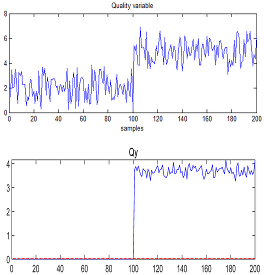
Figure 7. The quality variable and $Q_y$ statistic of $y$ under Fault 3 conditions.

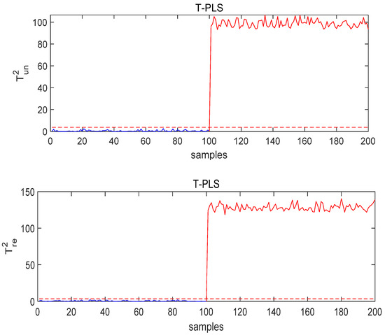
Figure 8. The monitoring results of T-PLS under Fault 3 conditions.

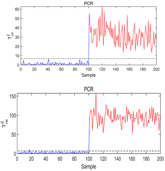
Figure 9. The monitoring results of PCR under Fault 3 conditions.

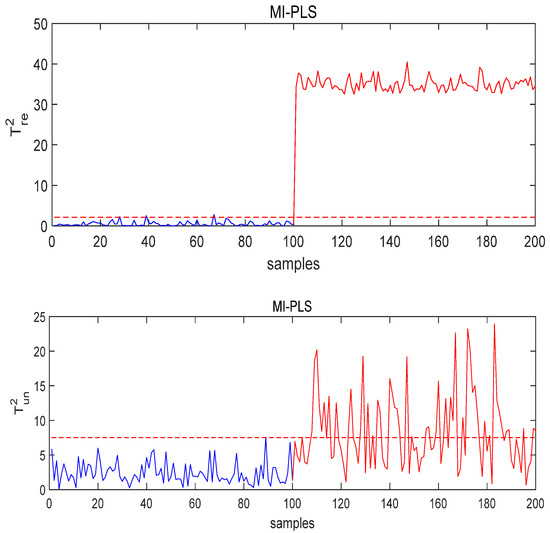
Figure 10. The monitoring results of MI-PLS under Fault 3 conditions.

Figure 8 and Figure 9 show the monitoring results under quality-related fault using the T-PLS algorithm and PCR, respectively. It can be seen from the results that although the fault is detected, both quality-related and quality-unrelated monitoring indices exceeded the threshold. By contrast, the MI-PLS algorithm proposed in this paper successfully detected the quality-related fault and the quality-unrelated indicator $T_{un}^2$ did not seriously exceed the threshold, as can be seen in Figure 10.

The false alarm rate (FAR) and fault detection rate (FDR) for TPLS, PCR, and MI-PLS are shown in Table 1, Table 2 and Table 3. For faults related to quality, the false alarm rate (FAR) should be as low as possible. The statistical indicators should not exceed the threshold in the case of a fault not related to quality.

Table 1. False alarm rate (FAR) for faults not related to quality using quality-related statistical indicators.

Fault No.	PCR ${\mathit{T}}_{\mathit{r}\mathit{e}}^2$	T-PLS ${\mathit{T}}_{\mathit{r}\mathit{e}}^2$	MI-PLS ${\mathit{T}}_{\mathit{r}\mathit{e}}^2$
1	40%	55%	0%
2	48%	46%	2%

Table 2. Fault detection rate (FDR) for faults not related to quality using quality-unrelated statistical indicators (%).

Fault No.	PCR ${\mathit{T}}_{\mathit{u}\mathit{n}}^2$	T-PLS ${\mathit{T}}_{\mathit{u}\mathit{n}}^2$	MI-PLS ${\mathit{T}}_{\mathit{u}\mathit{n}}^2$
1	100%	100%	100%
2	98%	100%	100%

Table 3. Fault detection rate (FDR) for quality-related faults using quality-related statistical indicators.

Fault No.	PCR ${\mathit{T}}_{\mathit{r}\mathit{e}}^2$	T-PLS ${\mathit{T}}_{\mathit{r}\mathit{e}}^2$	MI-PLS ${\mathit{T}}_{\mathit{r}\mathit{e}}^2$
3	99%	100%	100%
4	82.5%	96%	100%

For both quality-related faults and faults unrelated to quality, the proposed MI-PLS approach achieved the best overall result. However, in order to closely follow the monitoring performance of this method and verify that it can monitor the fault conditions of quality variables in real time, we carried out the two simulations using the same high configuration computer and recorded running times of 4.13 and 3.26 s for T-PLS and MI-PLS, respectively. MI-PLS has a lower computational load requirement than T-PLS.

4.2. Tennessee Eastman Process Simulation

The Tennessee Eastman process (TEP) was originally a real chemical process built by Eastman Chemical Company. Later, Downs et al. [25] developed the chemical test experimental platform based on the actual reaction process, which has been successfully used to test and evaluate the performance of process control strategies and various monitoring algorithms. After years of research and application, it has become a standard test platform in the field of quality monitoring. The flowchart for the process is shown in Figure 11 [25].

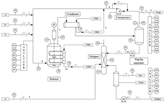
Figure 11. Schematic of the Tennessee Eastman (TE) process.

The TE process simulator contains five main units: the compressor, reactor, stripper, condenser, and separator. The input reactants include five components—A, B, C, D, E—and the quality variables G and H. In this industrial process, all 53 process variables are divided into two parts: 41 measured variables and 12 manipulated variables. In this experiment, the output variables are XMEAS 35 and 36, which are the measurement values of product components H and G. The process variable $X$ matrix contains two sections: 22 measured variables (XMEAS 1–22) and 11 manipulated variables (XMV 1–11). These input variables are listed in Table 4.

Table 4. The description of process variables in the $X$ matrix.

Variable No.	Variable Name
XMV 1	D feed flow
XMV 2	E feed flow
XMV 3	A feed flow
XMV 4	A and C feed flow
XMV 5	Compressor recycle valve
XMV 6	Purge valve
XMV 7	Separator pot liquid flow
XMV 8	Stripper liquid product flow
XMV 9	Stripper steam valve
XMV 10	Reactor cooling water flow
XMV 11	Condenser cooling water flow
XMEAS 1	A feed
XMEAS 2	D feed
XMEAS 3	E feed
XMEAS 4	A and C feed
XMEAS 5	Recycle flow
XMEAS 6	Reactor feed rate
XMEAS 7	Reactor pressure
XMEAS 8	Reactor level
XMEAS 9	Reactor temperature
XMEAS 10	Purge rate
XMEAS 11	Product separator temperature
XMEAS 12	Product separator level
XMEAS 13	Product separator pressure
XMEAS 14	Product separator underflow
XMEAS 15	Stripper level
XMEAS 16	Stripper pressure
XMEAS 17	Stripper underflow
XMEAS 18	Stripper temperature
XMEAS 19	Stripper steam flow
XMEAS 20	Compressor work
XMEAS 21	Reactor cooling water outlet temperature
XMEAS 22	Separator cooling water outlet temperature

The sampling interval for measurement was set at 3 min. Then, Simulink codes were used to produce fifteen datasets. One dataset was produced under normal operation, and the other datasets corresponded to fourteen different faults. These faults are listed in Table 5.

Table 5. Description of fourteen fault types used in this study.

Fault No.	Process Variable	Type
IDV 1	A/C feed ratio, B composition constant	Step
IDV 2	B composition, A/C ratio constant	Step
IDV 3	D feed temperature	Step
IDV 4	Reactor cooling water inlet temperature	Step
IDV 5	Condenser cooling water inlet temperature	Step
IDV 6	A feed loss	Step
IDV 7	C header pressure loss-reduced availability	Step
IDV 8	A, B, C feed composition	Random variation
IDV 9	D feed temperature	Random variation
IDV 10	C feed temperature	Random variation
IDV 11	Reactor cooling water inlet temperature	Random variation
IDV 12	Condenser cooling water inlet temperature	Random variation
IDV 13	Reaction kinetics	Slow drift
IDV 14	Reactor cooling water valve	Sticking
IDV 15	Condenser cooling water valve	Sticking
IDV 16	Unknown	Unknown
IDV 17	Unknown	Unknown
IDV 18	Unknown	Unknown
IDV 19	Unknown	Unknown
IDV 20	Unknown	Unknown
IDV 21	The valve of stream 4 set in a constant position	Constant Position

According to the prior knowledge of these faults, there were ten quality-related faults (IDV 1, 2, 5–8, 12, 13, 18, and 21) and eleven faults unrelated to quality (IDV 3, 4, 9–11, 14, 15, 16, 17, 19 and 20). The prediction result is a suitable way to illustrate the model’s accuracy. In this experiment, to verify the predictive ability of MI-PLS, the quality variable XMEAS (35) was selected as the true value. For fair comparison, 16 latent variables for the two methods were selected. The confidence level was 99% when computing the limit of each monitoring index.

Figure 12 shows the predicted and true values using the MI-PLS algorithm under normal (fault free) conditions. The prediction accuracy of MI-PLS is very high, for example, comparing the mean and STD between the predicted series and the actual output series, the means are 17.301 and 16.912, respectively, and STD are 5.91 and 5.72, respectively. Afterwards, the MI-PLS algorithm was tested with quality-related Fault 8, and Fault 14, which was not related to quality.

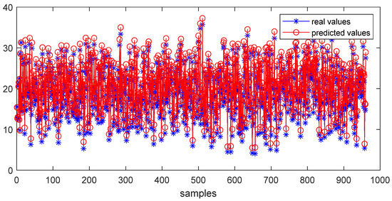
Figure 12. The prediction result of MI-PLS under fault-free conditions.

3.

Case study of Fault 14

Fault 14 consists of a sticking fault on the reactor cooling water valve. Figure 13 shows that the output variable has not changed. It shows almost no change before and after the fault occurs, and always remains within the normal range. Thus, Fault 14 is not related to quality.

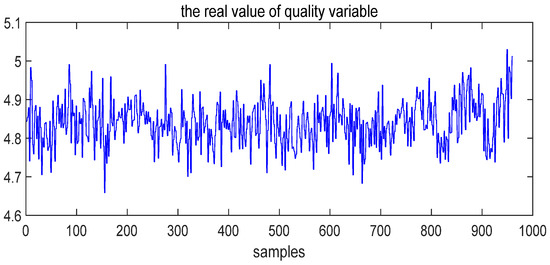
Figure 13. The real value of the quality variable under Fault 14 conditions.

Figure 14, Figure 15 and Figure 16 show the monitoring results for Fault 14 using T-PLS, PCR, and MI-PLS, respectively. As shown in Figure 14 and Figure 15, although T-PLS and PCR can detect this fault successfully, the quality-related monitoring statistics exceed the control limit, which is not in line with the actual situation. By contrast, the quality-related monitoring statistic of MI-PLS does not exceed the threshold, as seen in Figure 16, which reflects the true situation. The quality variable maintains a normal status, so no alarm should occur here. Thus, for this fault condition, it is logical that the statistic relevant to quality is below the threshold.

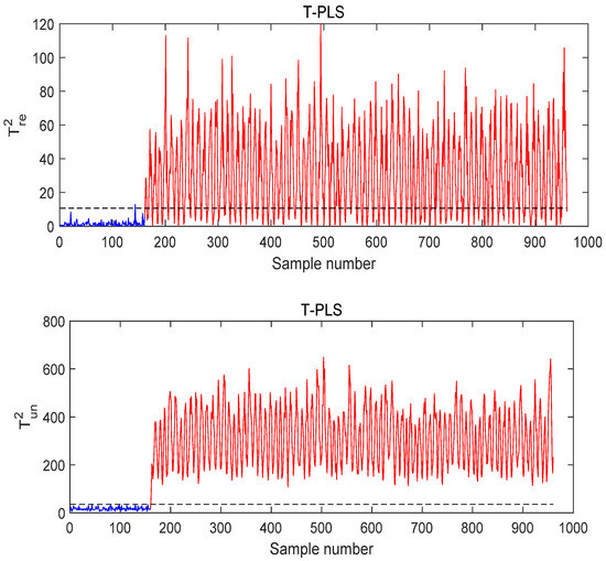
Figure 14. The monitoring result of MI-PLS under Fault 14 conditions.

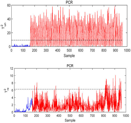
Figure 15. The monitoring result of PCR under Fault 14 conditions.

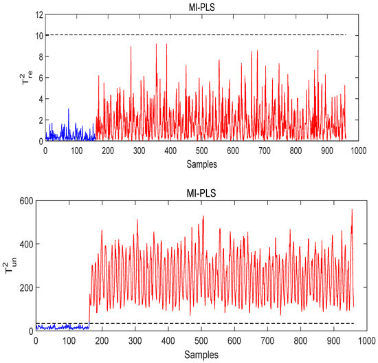
Figure 16. The monitoring result of MI-PLS under Fault 14 conditions.

From these results, it can be concluded that the advantage of the method proposed in this paper is in achieving the lowest false alarm rates in the case of faults unrelated to quality. Due to the effective quality variable selection method we used in this algorithm, the false alarm rate (FAR) of MI-PLS is close to 0%. Using the PCR and T-PLS methods, the false alarm rate (FAR) is higher, e.g., in T-PLS, it reached 62.5%, which leads to needless stops and reconditioning.

4.

Case Study of Fault 8

Fault 8 consists of a random variation in the feed composition. From Figure 17, it can be seen that the quality variable was affected after the fault occurred; this means the fault is quality-related. The monitoring results of T-PLS, PCR, and M-PLS under Fault 8 are shown in Figure 18, Figure 19 and Figure 20.

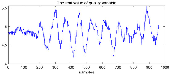
Figure 17. The real value of the quality variable under fault 8.

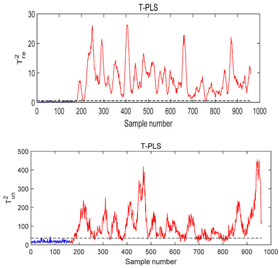
Figure 18. The monitoring result of T-PLS under Fault 8 conditions.

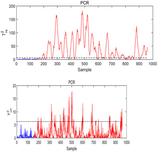
Figure 19. The monitoring result of PCR under Fault 8 conditions.

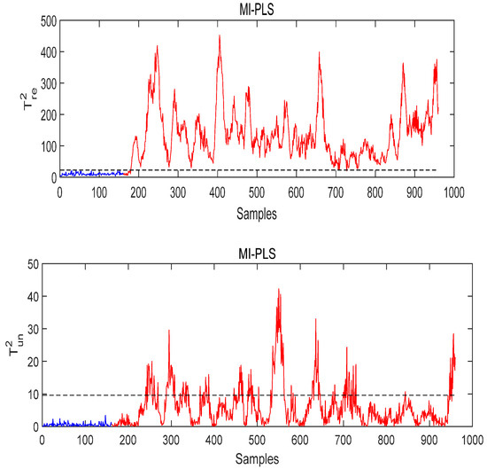
Figure 20. The monitoring result of MI-PLS under Fault 8 conditions.

Figure 18 and Figure 19 are the monitoring results using T-PLS and PCR, respectively. As can be seen, both the T-PLS and PCR algorithms lead to a low fault detection rate (FDR). Using MI-PLS, the monitoring statistics exceed the control limit after the fault occurs and stays above the control limit, as shown in Figure 20. Besides, the quality-unrelated monitoring statistics in both the T-PLS and PCR exceed the threshold, while in MI-PLS, it does not seriously exceed it. The fault detection rate (FDR) in MI-PLS reaches 99%, while for PCR and T-PLS the FDR is 82.75% and 97.5, respectively. Therefore, MI-PLS achieved the best results in detecting Fault 8.

From these results, it can be concluded that the proposed MI-PLS outperforms the other two methods in quality-related fault detection. The variable selection method we used in the proposed MI-PLS has a better variable filtering and variable selection ability, which means that if we use better variable selection methods with traditional methods, such as PCR, PLS or ICR, we may obtain better monitoring results.

Finally, the fault detection rates (FDRs) of quality-related faults of the proposed method and DPCA are listed in Table 6; the proposed approach keeps a high FDR in most of the quality-related faults.

Table 6. Fault detection rate (FDR) of MI-PLS, PCR and T-PLS for faults related to quality in the Tennessee Eastman (TE) process.

Fault Number	PCR	T-PLS	MI-PLS
IDV 1	93.50%	89.35%	98.25%
IDV 2	67.65%	85.40%	96.25%
IDV 5	24.95%	95.20%	100%
IDV 6	97.50%	99.70%	99.40%
IDV 7	91.15%	90.30%	90.65%
IDV 8	82.75%	97.50%	99.00%
IDV 10	36.50%	26%	82.5%
IDV 12	97.50%	98.25%	98.25%
IDV 13	82.50%	93.20%	92.65%

Table 7 shows the false alarm rate (FAR) for faults unrelated to quality using the proposed MI-PLS, PCR and T-PLS methods. Our results show that the proposed MI-PLS algorithm has a lower FAR for most of the faults that were not related to quality.

Table 7. False alarm rate (FAR) for MI-PLS, PCR, and T-PLS with faults unrelated to quality in the TE process.

Fault Number	PCR	T-PLS	MI-PLS
3	9.75%	2.35%	0.75%
4	2.37%	8.18%	0.91%
9	1.25%	1.51%	2.90%
11	23.50%	7.01%	4.64%
14	60.74%	62.50%	0.00%
15	2.05%	2.50%	1.75%

5. Conclusions

In this article, a novel PLS based on the mutual information variable selection method was proposed. This method first utilizes mutual information (MI) to divide process variables into selected and residual parts, and then uses PLS to model the selected part and further decomposes this into quality-related and quality-unrelated parts, subsequently constructing monitoring statistics. With regard to the quality residual part, the proposed method does not ignore the residual, but performs PCA to obtain its score matrix and combines it with the quality-unrelated component of the selected part. It finally builds the total quality-unrelated statistical indicator. In this paper, a numerical example and the TE process were presented to test the proposed method and compare it with T-PLS and PCR. Numerical simulation experiments verify that the proposed MI-PLS model has a high degree of fit and can obtain more accurate prediction results. Through the experimental comparison of the numerical simulation and TE benchmark platform, it is concluded that the proposed MI-PLS method has an improved detection of fault conditions and can effectively distinguish whether a fault affects product quality in real time, reducing the rate of missed alarms and false alarms. The detection results obtained here are more in line with the actual situation, verifying the effectiveness of MI-PLS in quality-related and quality-unrelated fault detection.

References

- Chiang, L.H.; Russell, E.L.; Braatz, R.D. Fault Detection and Diagnosis in Industrial Systems; Springer Science & Business Media: Berlin/Heidelberg, Germany, 2000. [Google Scholar]
- Joe Qin, S. Statistical process monitoring: Basics and beyond. J. Chemom. J. Chemom. Soc. 2003, 17, 480–502. [Google Scholar] [CrossRef]
- Tao, Y.; Shi, H.; Song, B.; Tan, S. Parallel quality-related dynamic principal component regression method for chemical process monitoring. J. Process Control 2019, 73, 33–45. [Google Scholar] [CrossRef]
- Wang, G.; Jiao, J. Quality-related fault detection and diagnosis based on total principal component regression model. IEEE Access 2018, 6, 10341–10347. [Google Scholar] [CrossRef]
- Tao, Y.; Shi, H.; Song, B.; Tan, S. A novel dynamic weight principal component analysis method and hierarchical monitoring strategy for process fault detection and diagnosis. IEEE Trans. Ind. Electron. 2019, 67, 7994–8004. [Google Scholar] [CrossRef]
- Chen, L.; Liu, Q.; Wang, L.; Zhao, J.; Wang, W. Data-driven prediction on performance indicators in process industry: A survey. Acta Autom. Sin. 2017, 43, 944–954. [Google Scholar]
- Ge, Z. Review on data-driven modeling and monitoring for plant-wide industrial processes. Chemom. Intell. Lab. Syst. 2017, 171, 16–25. [Google Scholar] [CrossRef]
- Ding, S.X. Data-driven design of monitoring and diagnosis systems for dynamic processes: A review of subspace technique based schemes and some recent results. J. Process Control 2014, 24, 431–449. [Google Scholar] [CrossRef]
- Asorey-Cacheda, R.; Garcia-Sanchez, A.-J.; García-Sánchez, F.; García-Haro, J. A survey on non-linear optimization problems in wireless sensor networks. J. Netw. Comput. Appl. 2017, 82, 1–20. [Google Scholar] [CrossRef]
- Jiang, Q.; Yan, X. Quality-driven kernel projection to latent structure model for nonlinear process monitoring. IEEE Access 2019, 7, 74450–74458. [Google Scholar] [CrossRef]
- Yan, S.; Yan, X. Quality-driven autoencoder for nonlinear quality-and process-related fault detection based on least square regularization and enhanced statistic. Ind. Eng. Chem. Res. 2020, 59, 12136–12143. [Google Scholar] [CrossRef]
- Song, B.; Shi, H.; Tan, S.; Tao, Y. Multi-Subspace orthogonal canonical correlation analysis for quality-related plant wide process monitoring. IEEE Trans. Ind. Inform. 2020. [Google Scholar] [CrossRef]
- Sun, C.; Hou, J. An Improved Principal Component Regression for Quality-Related Process Monitoring of Industrial Control Systems. IEEE Access 2017, 5, 21723–21730. [Google Scholar] [CrossRef]
- Yin, S.; Ding, S.X.; Xie, X.; Luo, H. A Review on Basic Data-Driven Approaches for Industrial Process Monitoring. IEEE Trans. Ind. Electron. 2014, 61, 6418–6428. [Google Scholar] [CrossRef]
- Gang, L.; Qin, S.J.; Zhou, D. Geometric properties of partial least squares for process monitoring. Automatica 2010, 46, 204–210. [Google Scholar]
- Yin, S.; Wang, G.; Gao, H. Data-Driven Process Monitoring Based on Modified Orthogonal Projections to Latent Structures. IEEE Trans. Control Syst. Technol. 2016, 24, 1480–1487. [Google Scholar] [CrossRef]
- Ding, S.; Yin, S.; Peng, K.; Hao, H. A Novel Scheme for Key Performance Indicator Prediction and Diagnosis With Application to an Industrial Hot Strip Mill. IEEE Trans. Ind. Inform. 2013, 9, 2239–2247. [Google Scholar] [CrossRef]
- Ju, H.; Yin, S.; Gao, H.; Kaynak, O. A data-based KPI prediction approach for wastewater treatment processes. In Proceedings of the International Conference on Man & Machine Interfacing, Bhubaneswar, India, 17–19 December 2015. [Google Scholar]
- Yu, J. Multiway Gaussian Mixture Model Based Adaptive Kernel Partial Least Squares Regression Method for Soft Sensor Estimation and Reliable Quality Prediction of Nonlinear Multiphase Batch Processes. Ind. Eng. Chem. Res. 2012, 51, 13227–13237. [Google Scholar] [CrossRef]
- Jiang, Q.; Yan, X.; Yi, H.; Gao, F. Data-driven batch-end quality modeling and monitoring based on optimized sparse partial least squares. IEEE Trans. Ind. Electron. 2019, 67, 4098–4107. [Google Scholar] [CrossRef]
- Si, Y.; Wang, Y.; Zhou, D. Key-performance-indicator-related process monitoring based on improved kernel partial least squares. IEEE Trans. Ind. Electron. 2020, 68, 2626–2636. [Google Scholar] [CrossRef]
- Fan, S.-K.S.; Chang, Y.-J. Multiple-input multiple-output double exponentially weighted moving average controller using partial least squares. J. Process Control 2010, 20, 734–742. [Google Scholar] [CrossRef]
- Fan, S.-K.S.; Chang, Y.-J. An integrated advanced process control framework using run-to-run control, virtual metrology and fault detection. J. Process Control 2013, 23, 933–942. [Google Scholar] [CrossRef]
- Zhou, D.; Li, G.; Qin, S.J. Total projection to latent structures for process monitoring. AIChE J. 2010, 56, 168–178. [Google Scholar] [CrossRef]
- Downs, J.J.; Vogel, E.F. A plant-wide industrial process control problem. Comput. Chem. Eng. 1993, 17, 245–255. [Google Scholar] [CrossRef]
Publisher’s Note: MDPI stays neutral with regard to jurisdictional claims in published maps and institutional affiliations. |
© 2021 by the authors. Licensee MDPI, Basel, Switzerland. This article is an open access article distributed under the terms and conditions of the Creative Commons Attribution (CC BY) license (http://creativecommons.org/licenses/by/4.0/).