A Novel Mutual Information and Partial Least Squares Approach for Quality-Related and Quality-Unrelated Fault Detection

Abstract
:1. Introduction
2. Related Work
| Algorithm 1. The Description of NIPALS Algorithm, Nonlinear Iterative Partial Least Squares (NIPALS) Algorithm Description |
| Let , start. (1) Take any column in and record as . (2) Calculate the regression of each column in on , and get the regression matrix as . (3) Normalize and calculate the score vector for as . (4) Calculate the regression of each column in on , and get the load matrix of as . (5) Compute the new score vector for as . (6) If converges, go to step (7), otherwise return to step (2). (7) Calculate the load matrix of as . (8) Calculate the residual matrices for and as and , respectively. (9) Replace and with and , respectively, and let return to step (1); repeat the calculation until latent variables are extracted, that is, stop iteration at . |
3. Quality-Related and Quality-Unrelated Fault Detection Based on MI-PLS
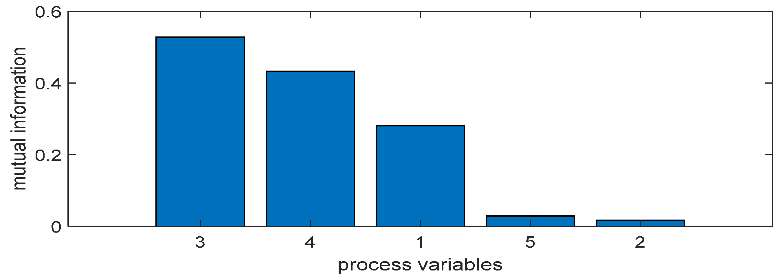
3.1. A Novel Quality Variables Selection Based on Mutual Information
3.2. The Proposed MI-PLS
- quality-related fault.
- no quality-related fault.
- quality-related or unrelated fault.
- no quality-unrelated fault.
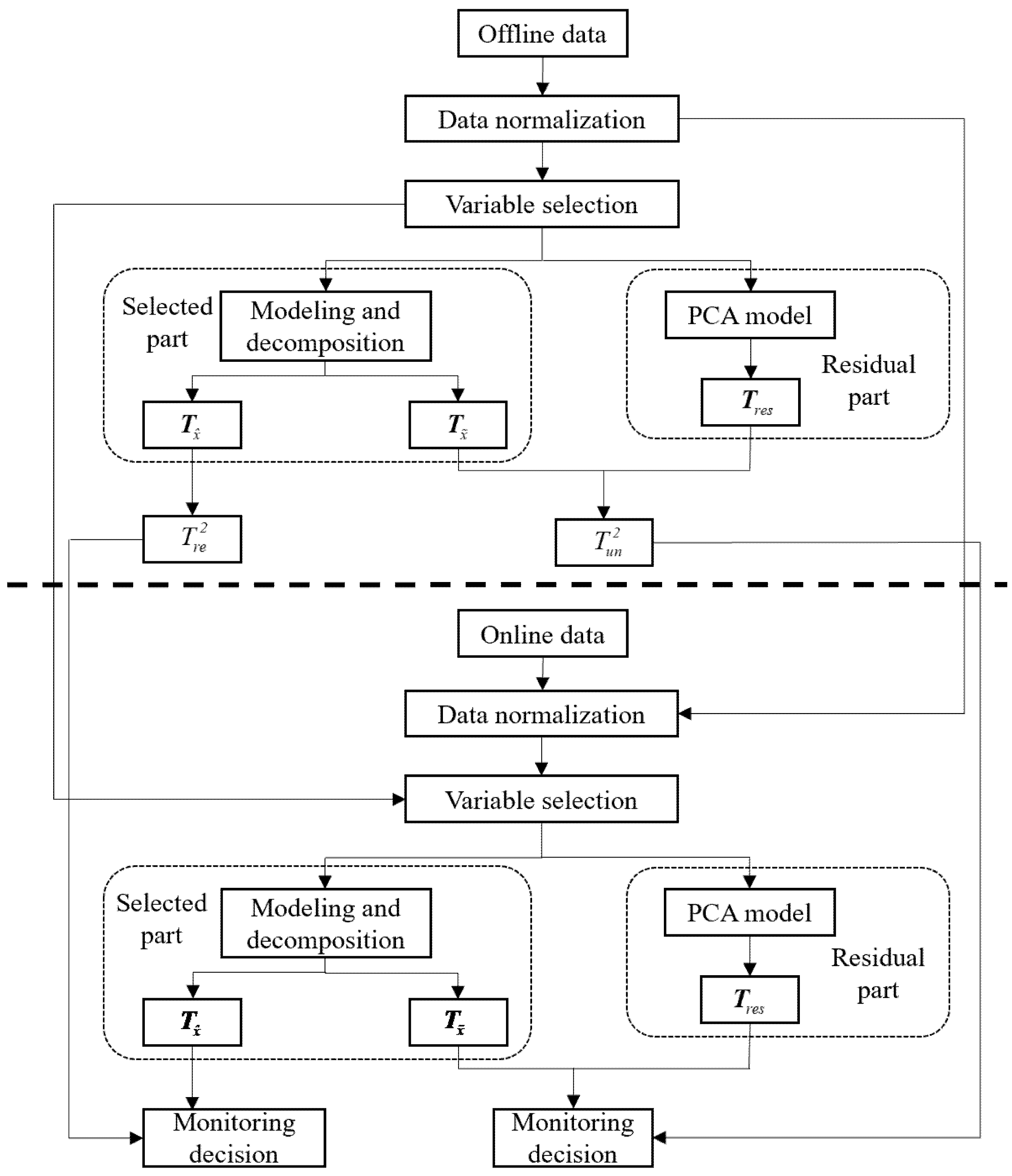
- Construct the offline process variable and quality variable matrices and ;
- Apply the proposed MI-based filtering method on the process variable matrix, , and quality variable matrix, , as summarized in Section 3.2. The filtered process variable matrix is denoted as . The loading and weight matrices are represented as and , respectively;
- Calculate the regression coefficient by performing standard PLS onto the filtered process data, , and quality data, , using the NIPALS in Algorithm 1;
- Perform SVD on to obtain and by (13);
- For each online test sample , correct it by ;
- Perform PCA on and combine with ;
- Calculate statistics and by (22) and (24), where is and is ;
- Calculate thresholds and by kernel density estimation (KDE);
- Diagnosis logic:
- quality-related fault has occurred;
- no quality-related fault has occurred;
- quality-related or unrelated fault has occurred;
- no fault unrelated to quality has occurred.
- MI-PLS requires few model latent variables; therefore, MI-PLS has a low computational load;
- MI-PLS utilizes the MI-based filtering method to remove variables that are irrelevant to quality before applying PLS. After this, it decomposes the selected part into quality-related and quality-unrelated subspaces in the postprocessing process; therefore, MI-PLS is more robust than other traditional methods;
- MI-PLS does not discard the residual, ; it participates in modeling and combines with unrelated parts from to ensure no information is lost.
4. Case Study
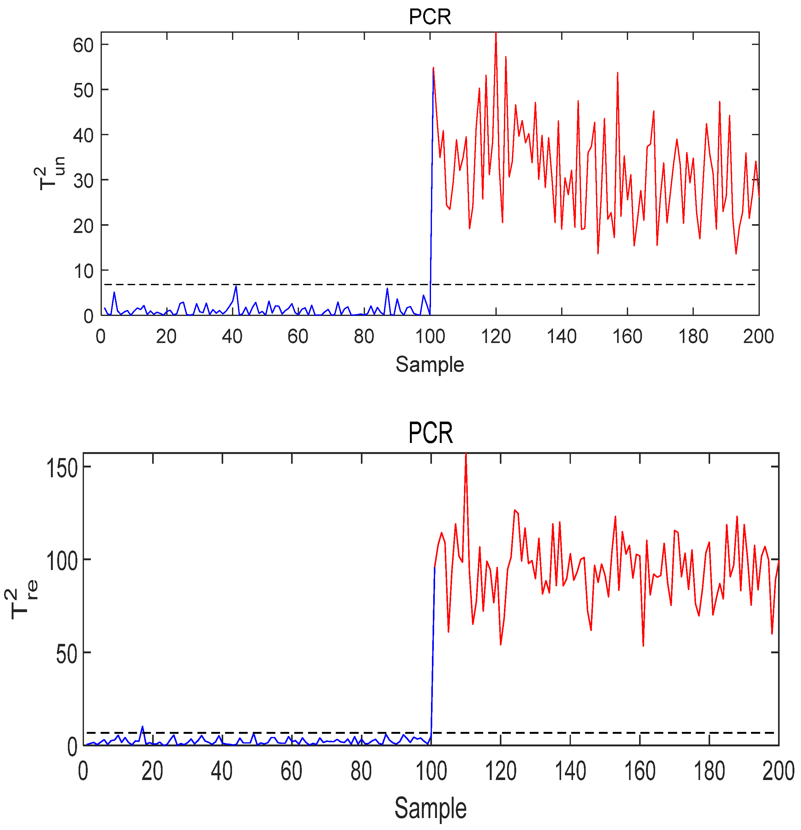
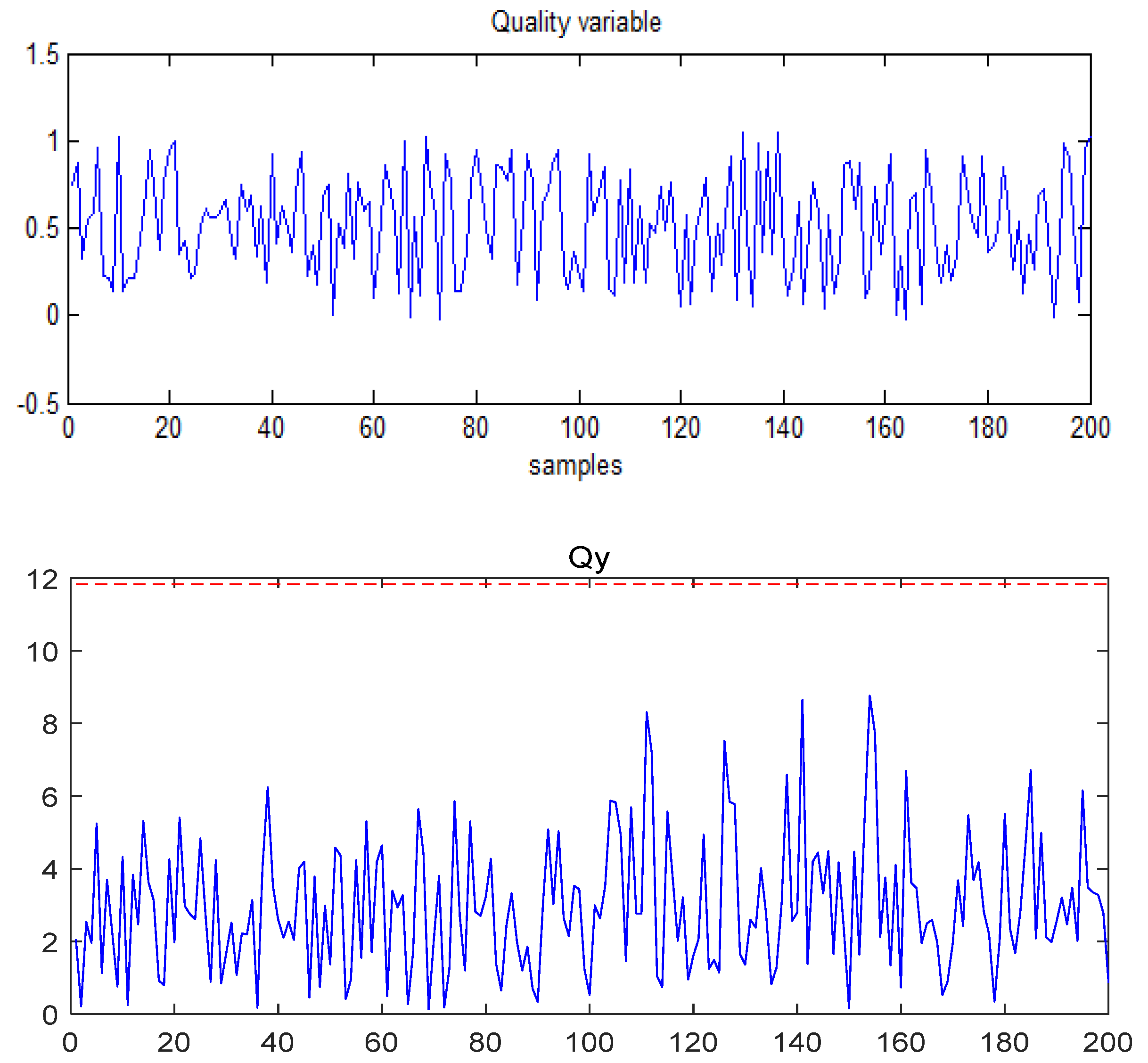
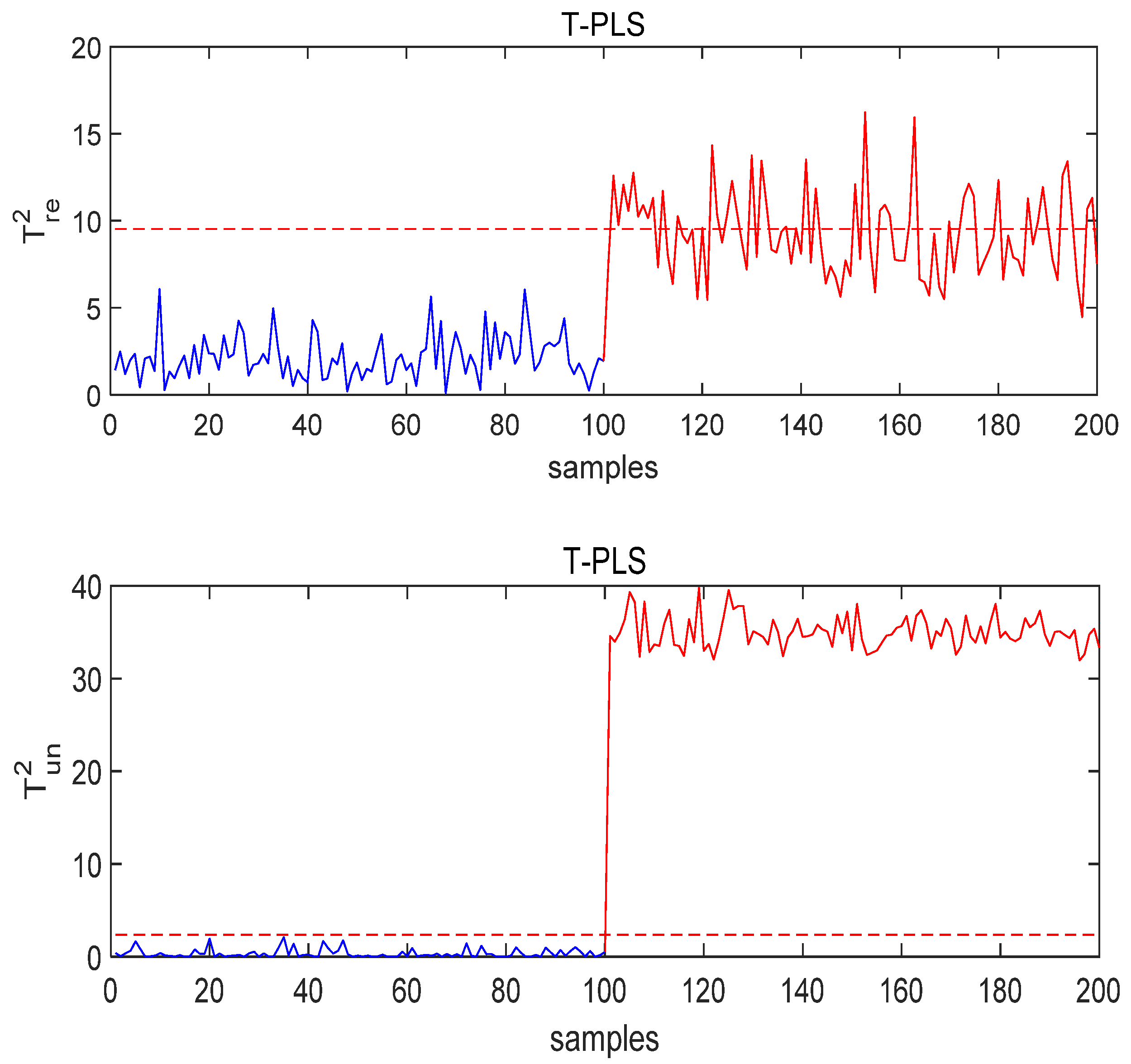
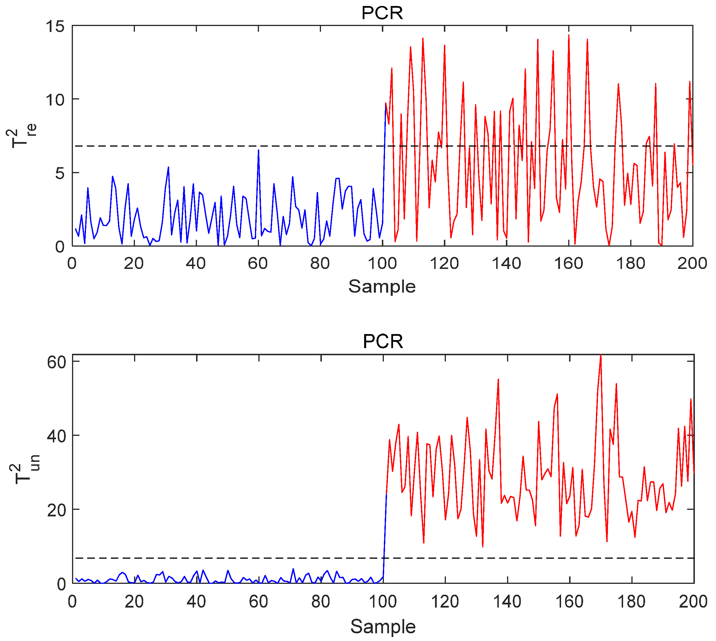
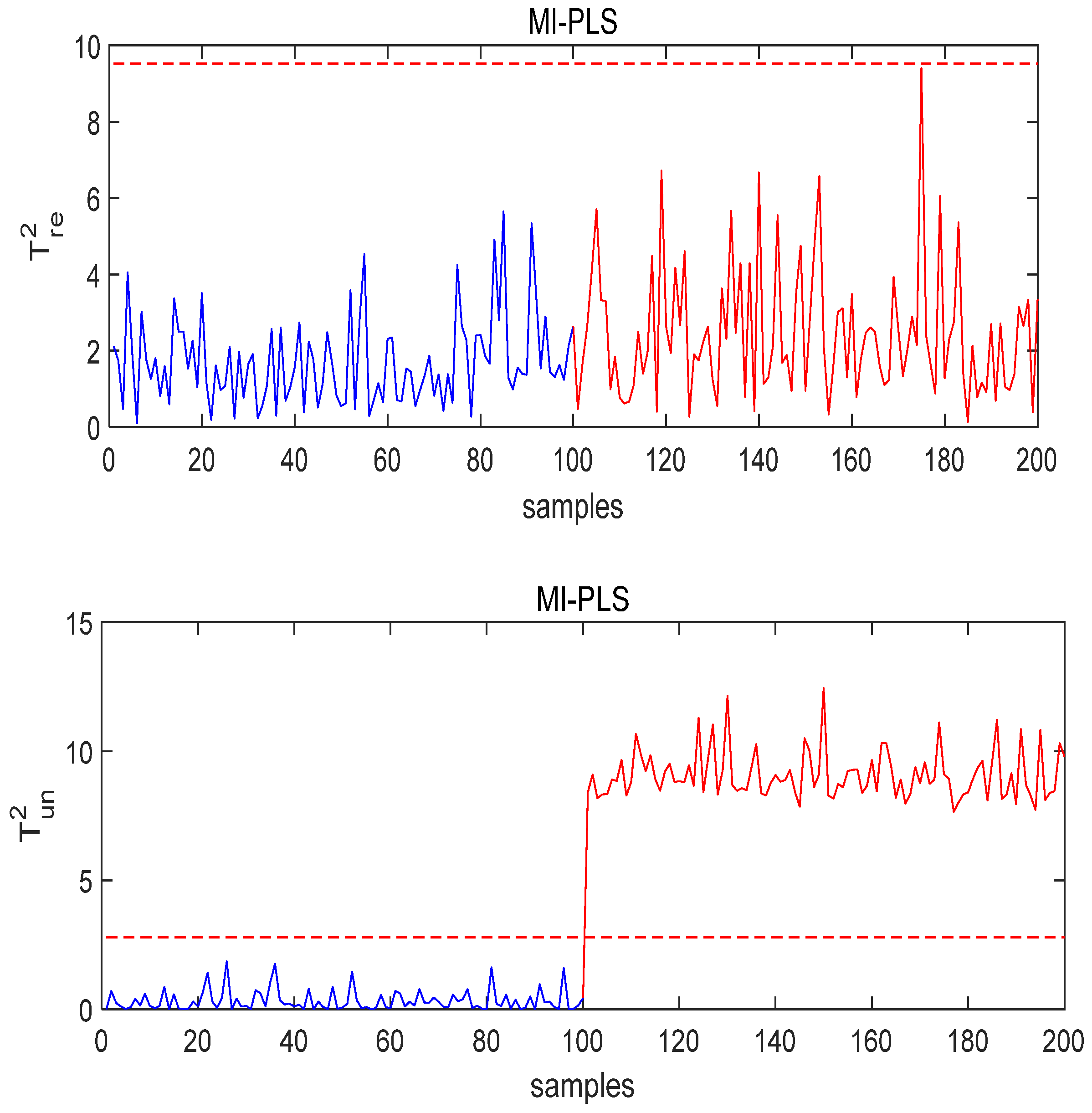
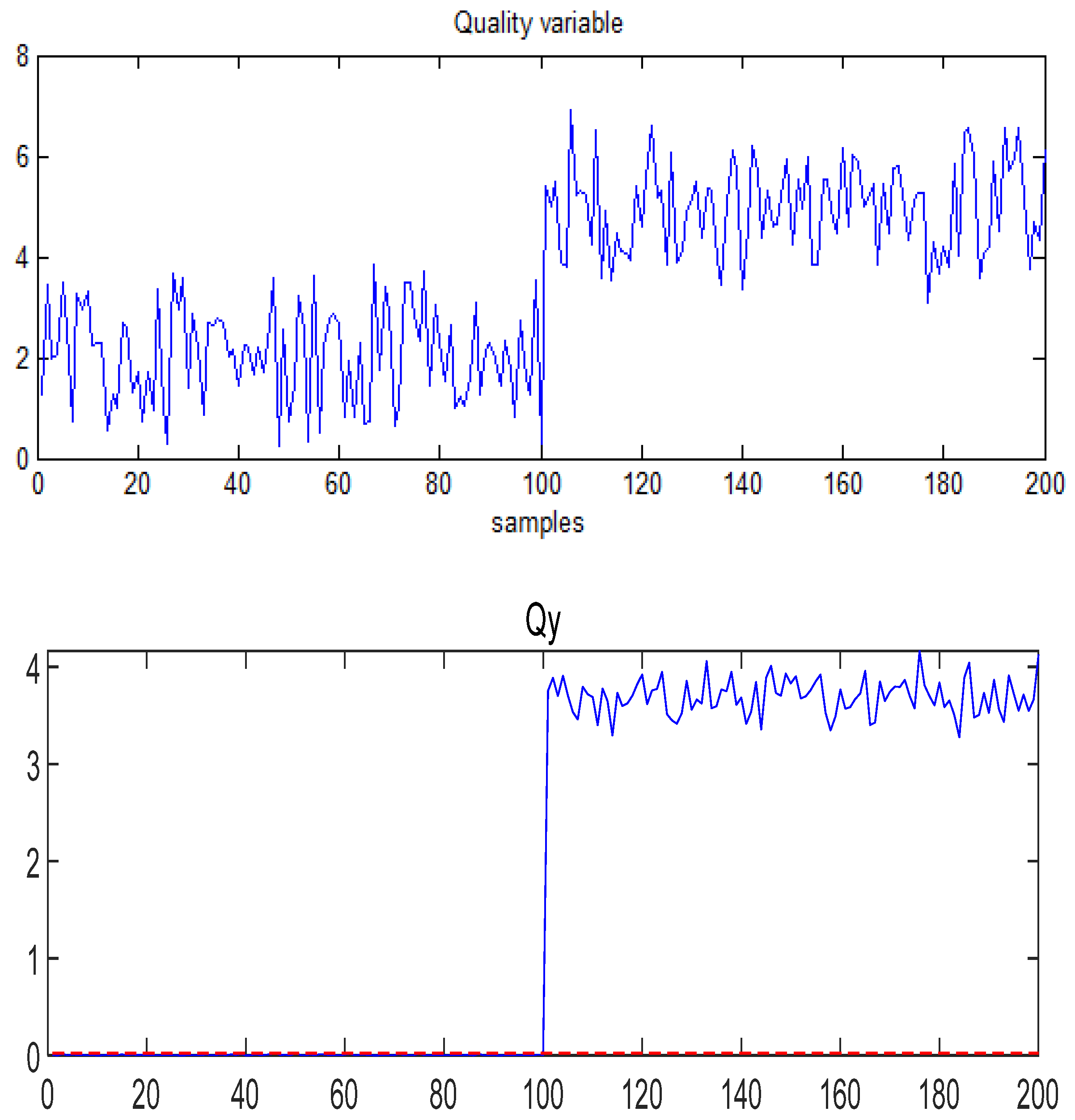
4.1. Numerical Example
- (1)
- With regard to quality-irrelevant faults, a low false-alarm rate in quality relevant monitoring statistics, and high fault-detection rate in quality-irrelevant monitoring statistics;
- (2)
- For quality-relevant faults, a high fault-detection rate in quality relevant monitoring statistics, but no specific requirement in relation to quality-irrelevant monitoring statistics.
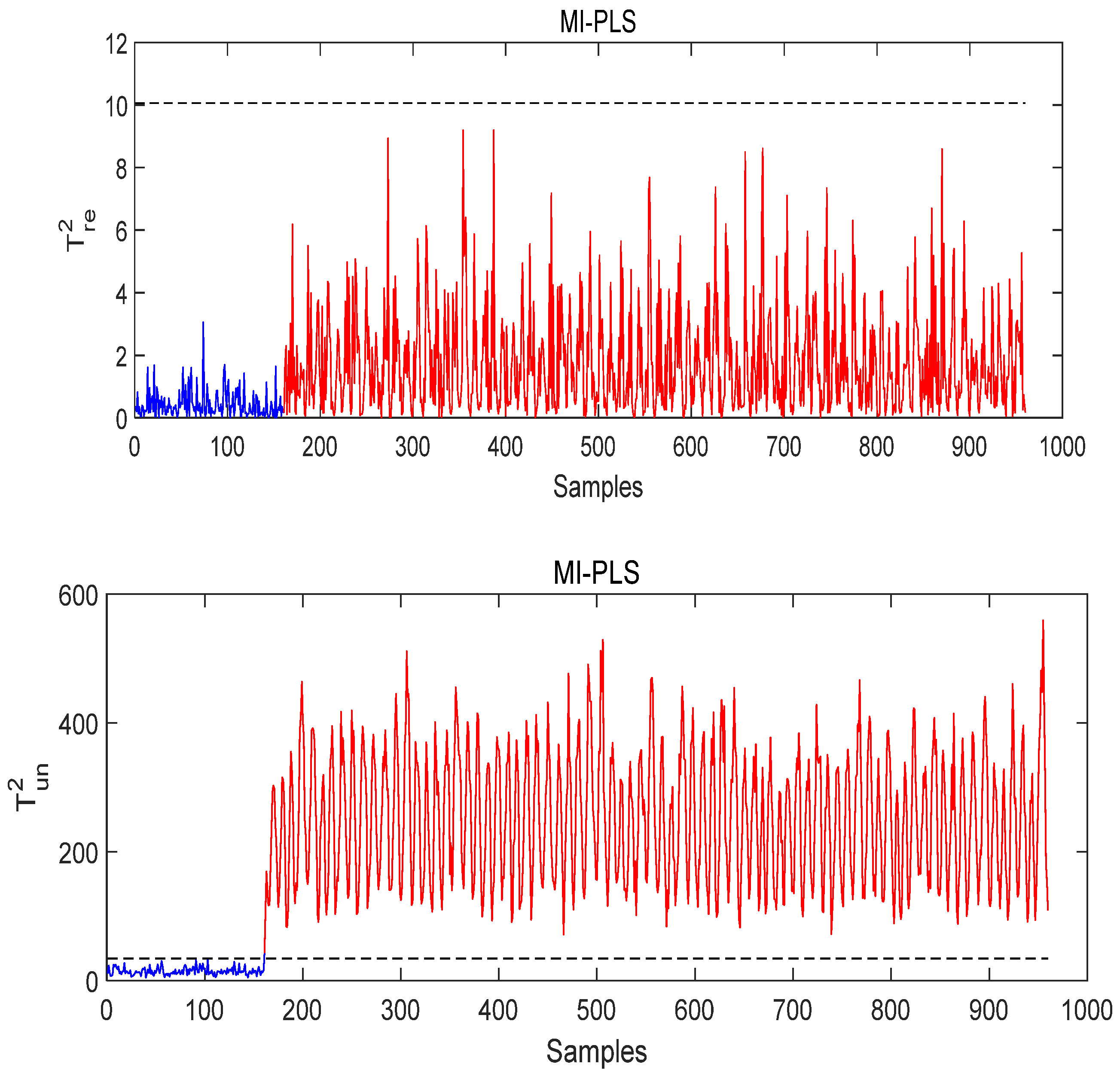
- Fault No.1: , quality-irrelevant;
- Fault No.2: , quality-irrelevant;
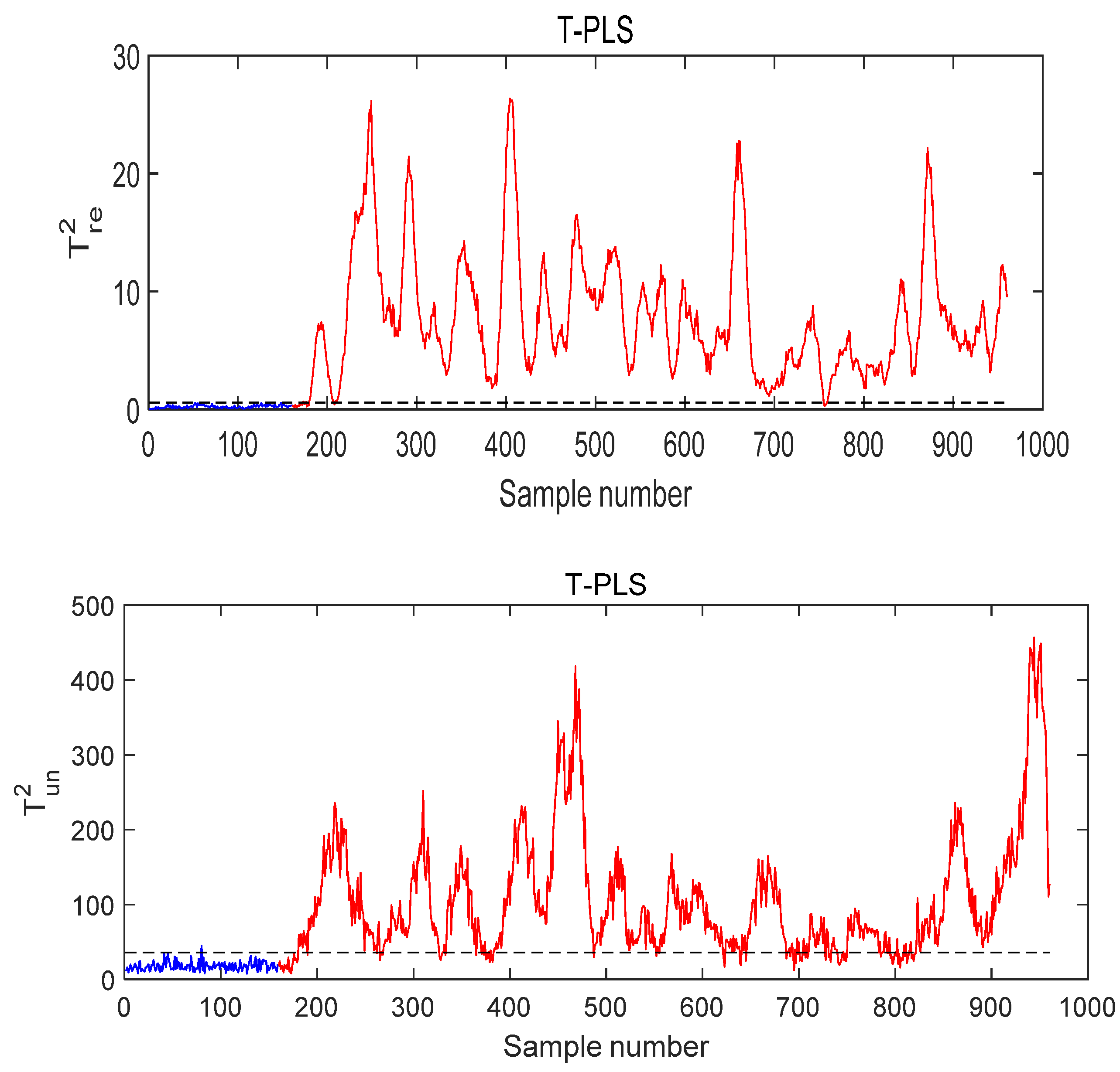
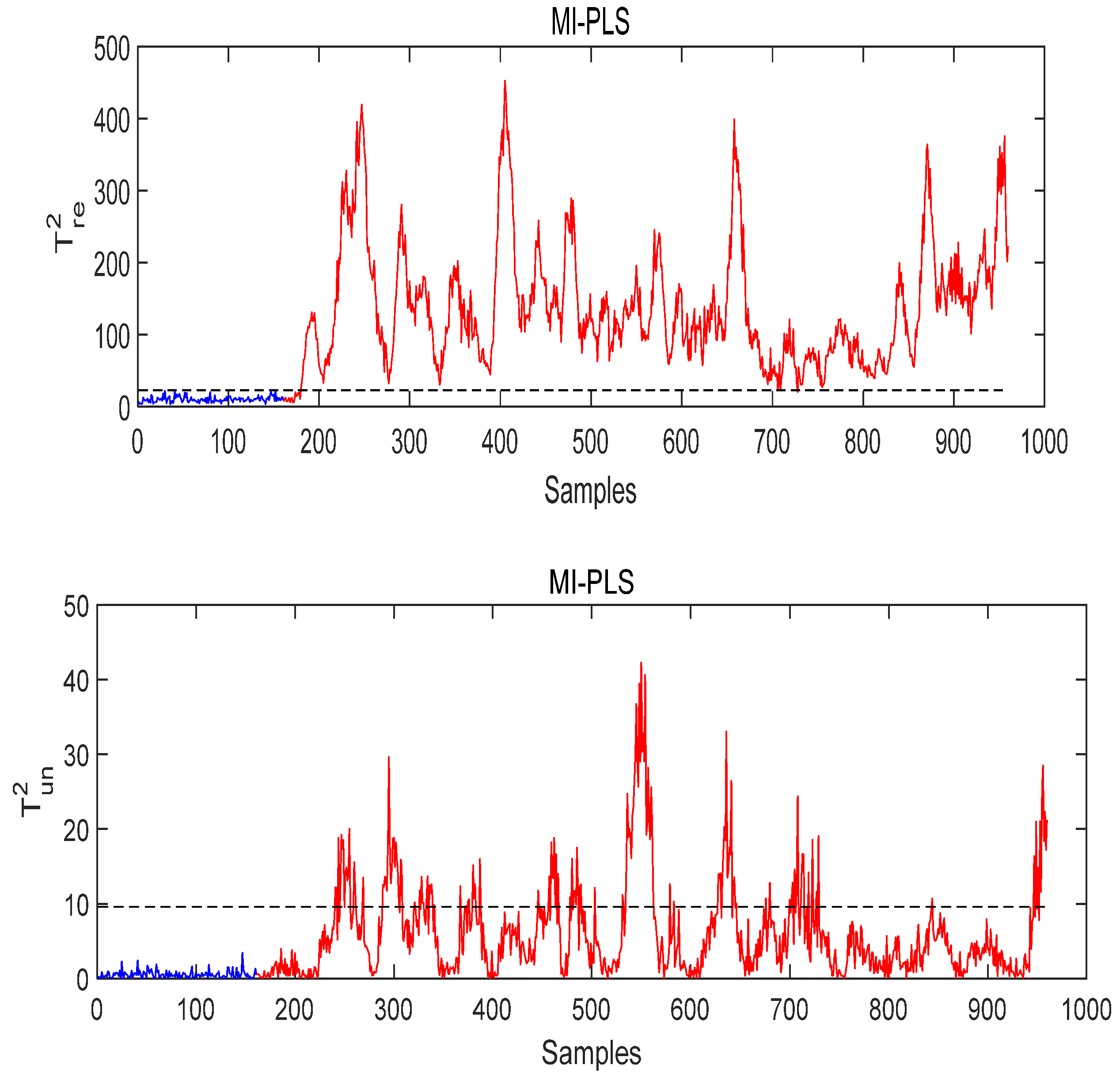
- Fault No.3: , quality-relevant;
- Fault No.4: , quality-relevant.
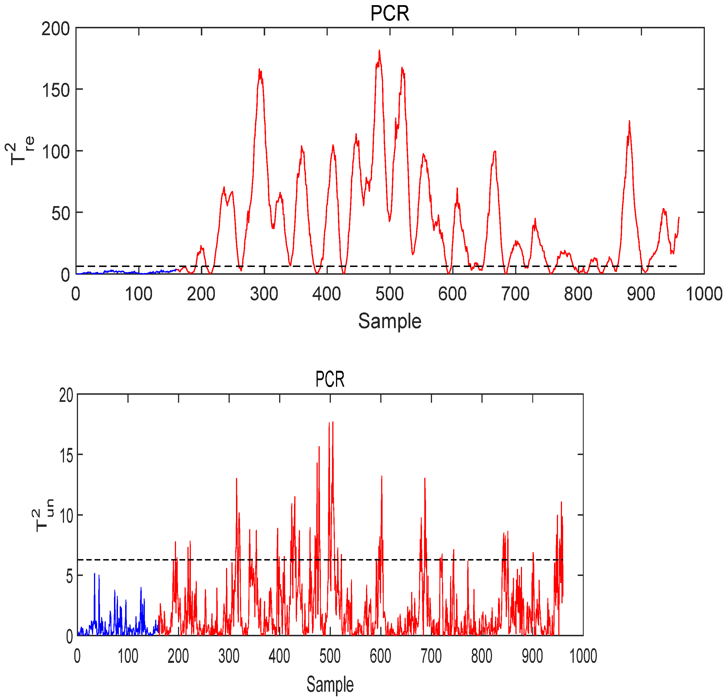
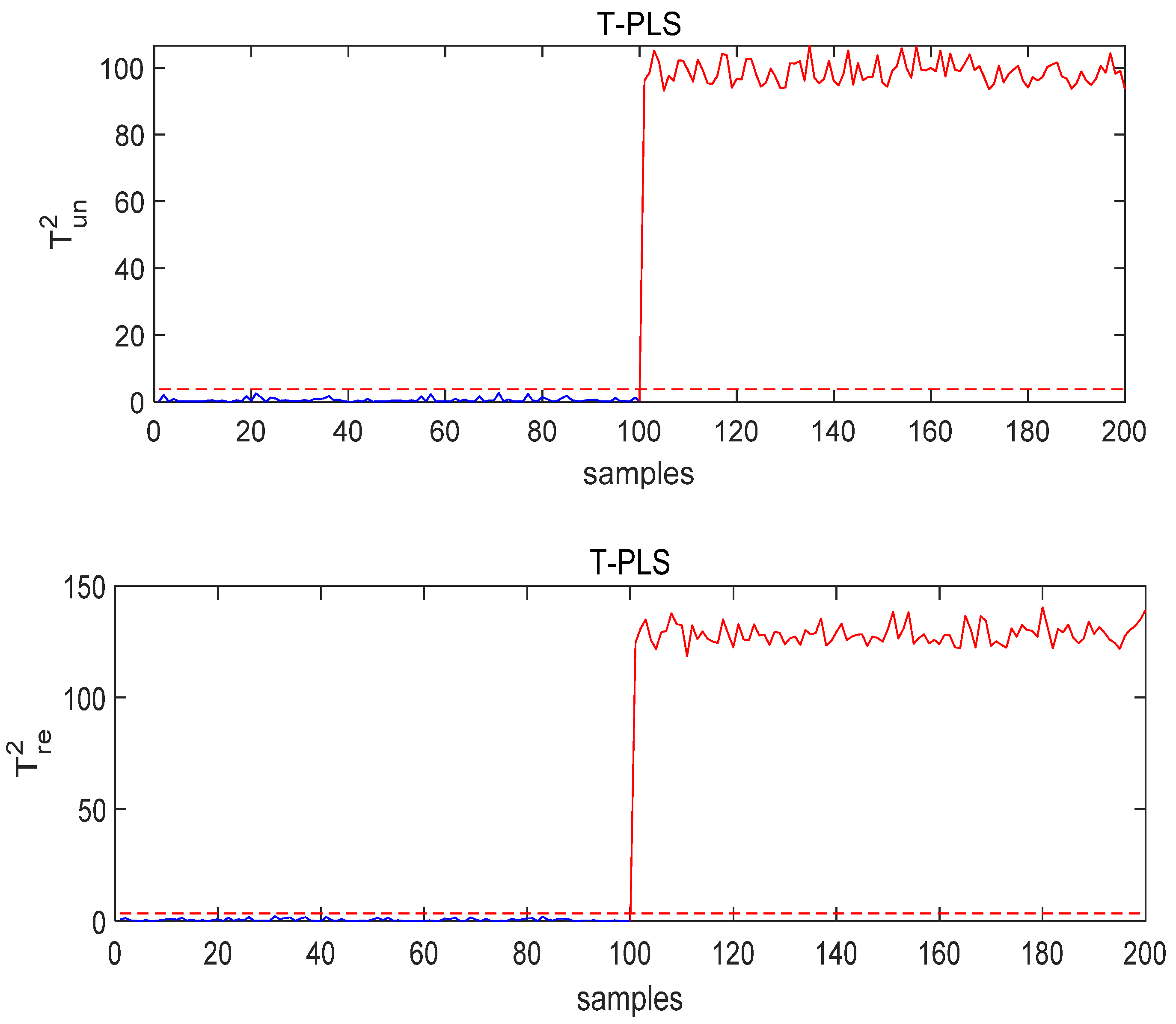
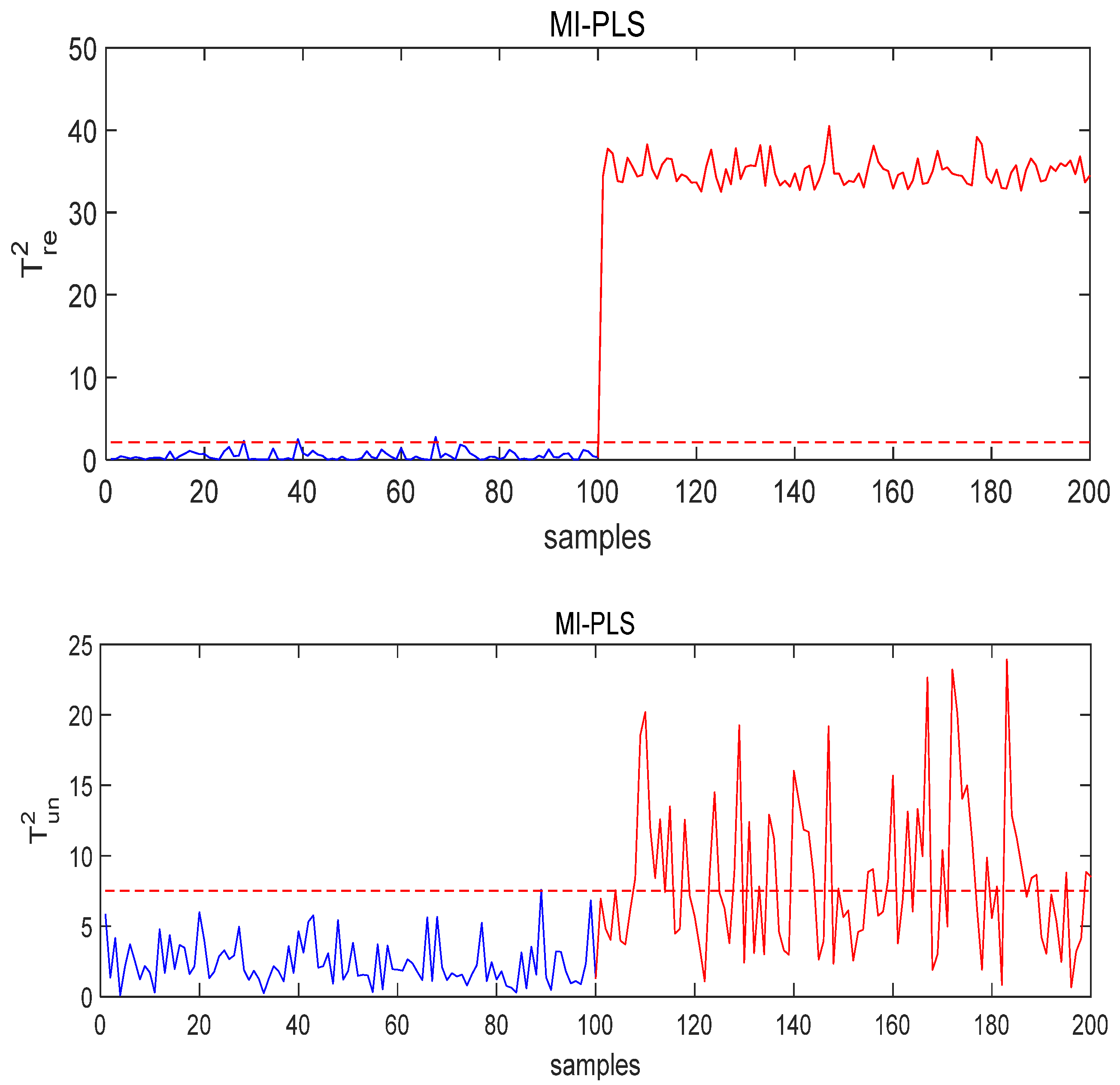
- Case study on Fault 1: The fault is added to
- 2.
- Case study on Fault 3: The fault is added to
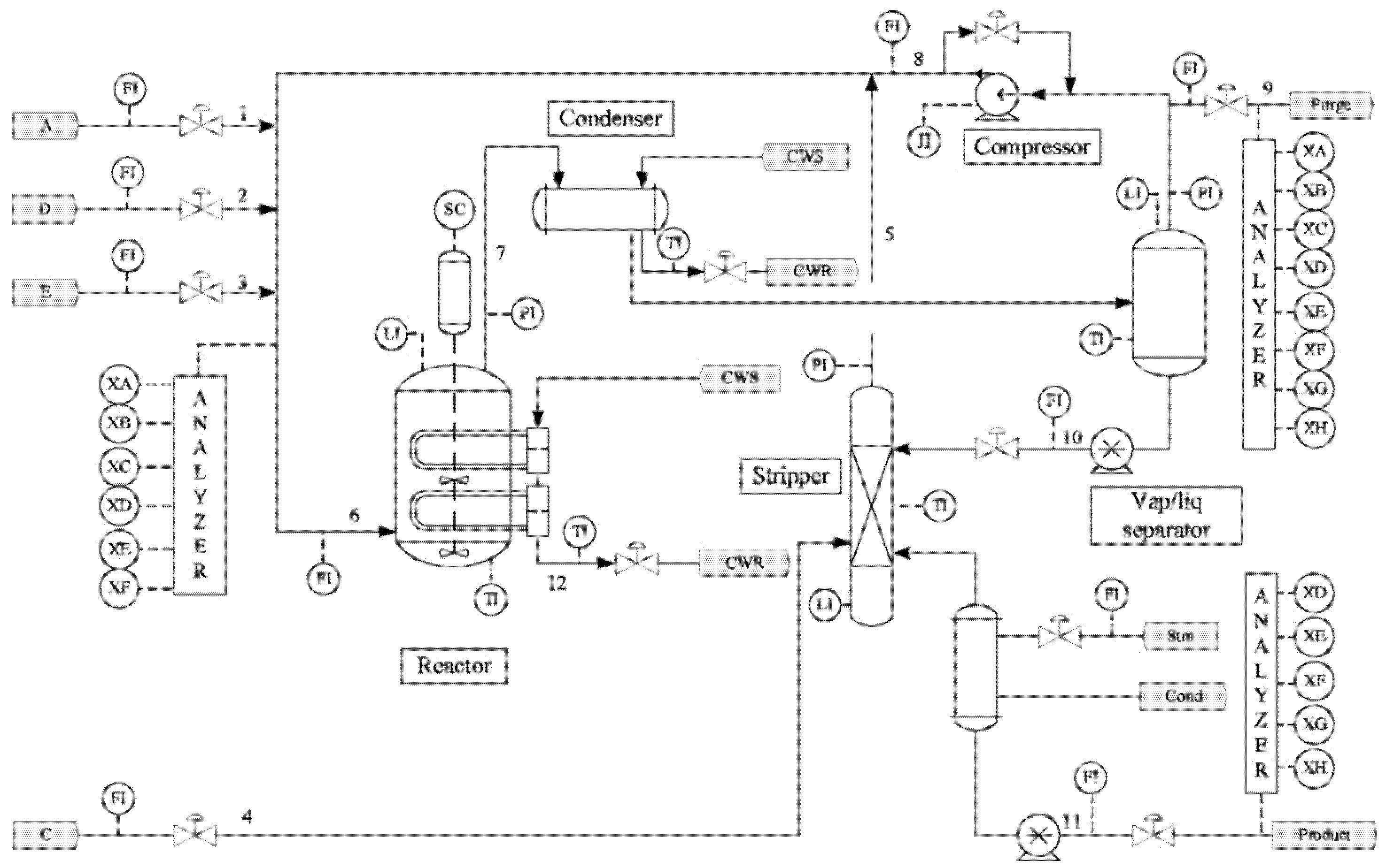
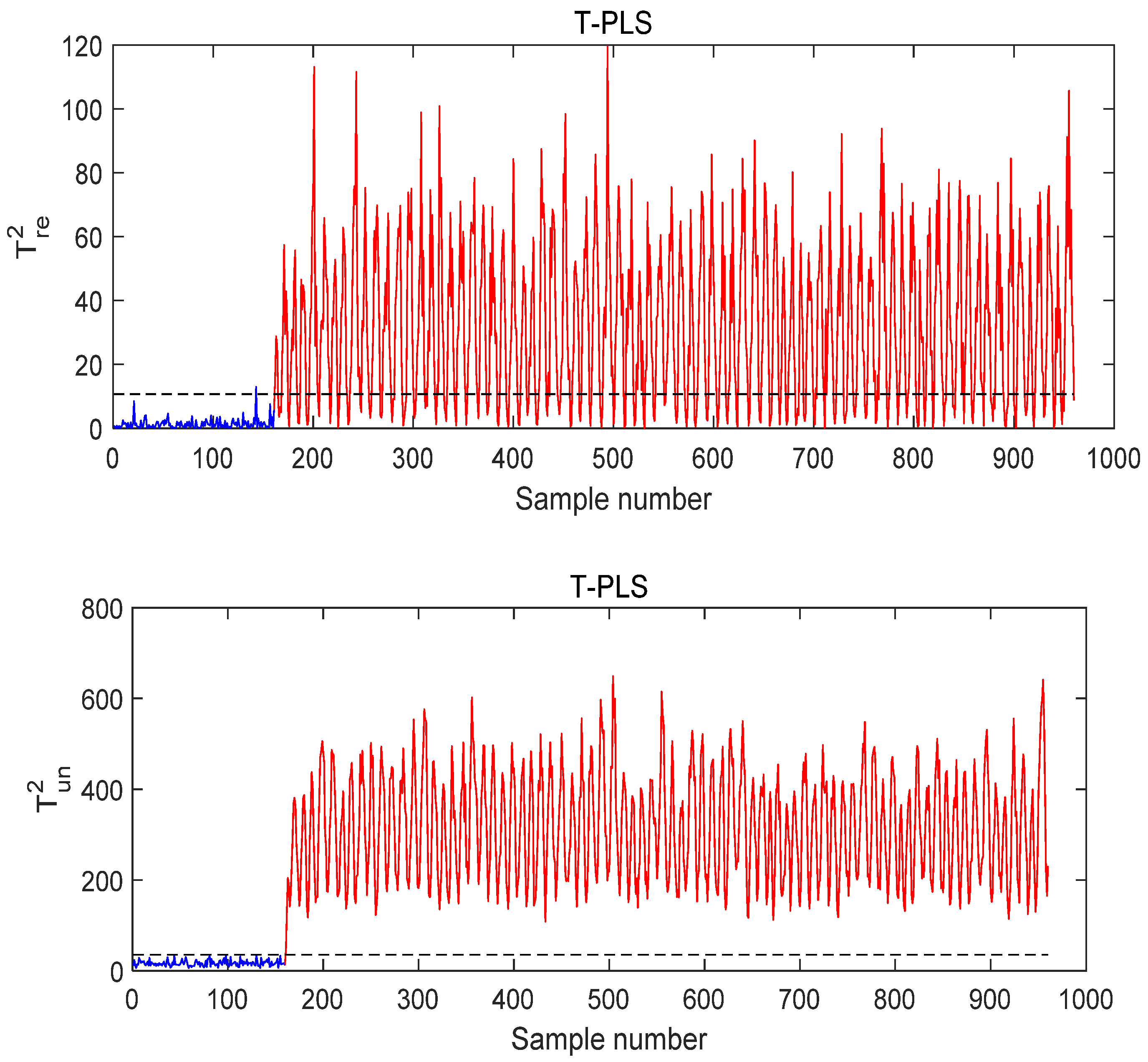
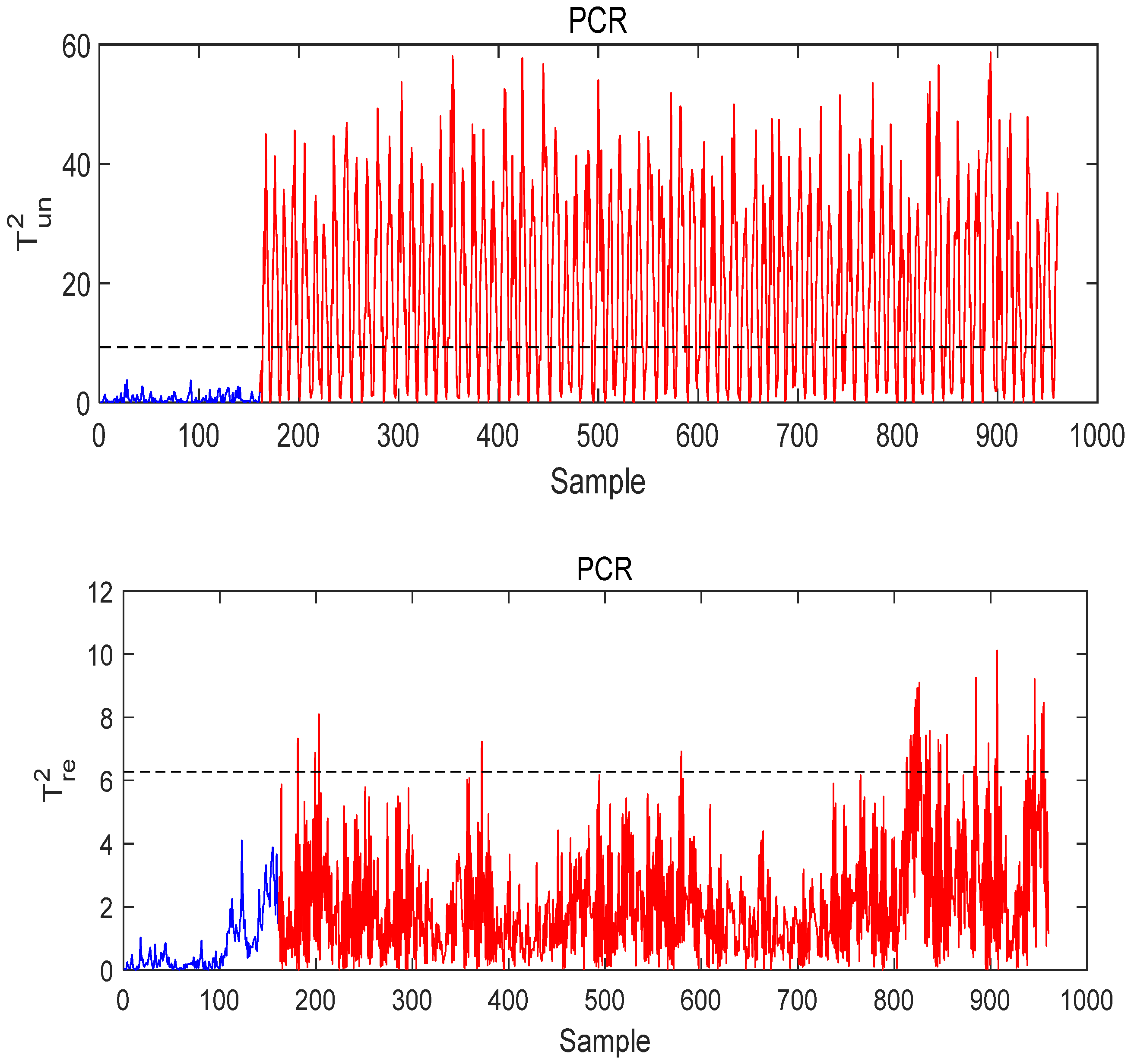
4.2. Tennessee Eastman Process Simulation
- 3.
- Case study of Fault 14
- 4.
- Case Study of Fault 8
5. Conclusions
Author Contributions
Funding
Institutional Review Board Statement
Informed Consent Statement
Data Availability Statement
Conflicts of Interest
References
- Chiang, L.H.; Russell, E.L.; Braatz, R.D. Fault Detection and Diagnosis in Industrial Systems; Springer Science & Business Media: Berlin/Heidelberg, Germany, 2000. [Google Scholar]
- Joe Qin, S. Statistical process monitoring: Basics and beyond. J. Chemom. J. Chemom. Soc. 2003, 17, 480–502. [Google Scholar] [CrossRef]
- Tao, Y.; Shi, H.; Song, B.; Tan, S. Parallel quality-related dynamic principal component regression method for chemical process monitoring. J. Process Control 2019, 73, 33–45. [Google Scholar] [CrossRef]
- Wang, G.; Jiao, J. Quality-related fault detection and diagnosis based on total principal component regression model. IEEE Access 2018, 6, 10341–10347. [Google Scholar] [CrossRef]
- Tao, Y.; Shi, H.; Song, B.; Tan, S. A novel dynamic weight principal component analysis method and hierarchical monitoring strategy for process fault detection and diagnosis. IEEE Trans. Ind. Electron. 2019, 67, 7994–8004. [Google Scholar] [CrossRef]
- Chen, L.; Liu, Q.; Wang, L.; Zhao, J.; Wang, W. Data-driven prediction on performance indicators in process industry: A survey. Acta Autom. Sin. 2017, 43, 944–954. [Google Scholar]
- Ge, Z. Review on data-driven modeling and monitoring for plant-wide industrial processes. Chemom. Intell. Lab. Syst. 2017, 171, 16–25. [Google Scholar] [CrossRef]
- Ding, S.X. Data-driven design of monitoring and diagnosis systems for dynamic processes: A review of subspace technique based schemes and some recent results. J. Process Control 2014, 24, 431–449. [Google Scholar] [CrossRef]
- Asorey-Cacheda, R.; Garcia-Sanchez, A.-J.; García-Sánchez, F.; García-Haro, J. A survey on non-linear optimization problems in wireless sensor networks. J. Netw. Comput. Appl. 2017, 82, 1–20. [Google Scholar] [CrossRef]
- Jiang, Q.; Yan, X. Quality-driven kernel projection to latent structure model for nonlinear process monitoring. IEEE Access 2019, 7, 74450–74458. [Google Scholar] [CrossRef]
- Yan, S.; Yan, X. Quality-driven autoencoder for nonlinear quality-and process-related fault detection based on least square regularization and enhanced statistic. Ind. Eng. Chem. Res. 2020, 59, 12136–12143. [Google Scholar] [CrossRef]
- Song, B.; Shi, H.; Tan, S.; Tao, Y. Multi-Subspace orthogonal canonical correlation analysis for quality-related plant wide process monitoring. IEEE Trans. Ind. Inform. 2020. [Google Scholar] [CrossRef]
- Sun, C.; Hou, J. An Improved Principal Component Regression for Quality-Related Process Monitoring of Industrial Control Systems. IEEE Access 2017, 5, 21723–21730. [Google Scholar] [CrossRef]
- Yin, S.; Ding, S.X.; Xie, X.; Luo, H. A Review on Basic Data-Driven Approaches for Industrial Process Monitoring. IEEE Trans. Ind. Electron. 2014, 61, 6418–6428. [Google Scholar] [CrossRef]
- Gang, L.; Qin, S.J.; Zhou, D. Geometric properties of partial least squares for process monitoring. Automatica 2010, 46, 204–210. [Google Scholar]
- Yin, S.; Wang, G.; Gao, H. Data-Driven Process Monitoring Based on Modified Orthogonal Projections to Latent Structures. IEEE Trans. Control Syst. Technol. 2016, 24, 1480–1487. [Google Scholar] [CrossRef]
- Ding, S.; Yin, S.; Peng, K.; Hao, H. A Novel Scheme for Key Performance Indicator Prediction and Diagnosis With Application to an Industrial Hot Strip Mill. IEEE Trans. Ind. Inform. 2013, 9, 2239–2247. [Google Scholar] [CrossRef]
- Ju, H.; Yin, S.; Gao, H.; Kaynak, O. A data-based KPI prediction approach for wastewater treatment processes. In Proceedings of the International Conference on Man & Machine Interfacing, Bhubaneswar, India, 17–19 December 2015. [Google Scholar]
- Yu, J. Multiway Gaussian Mixture Model Based Adaptive Kernel Partial Least Squares Regression Method for Soft Sensor Estimation and Reliable Quality Prediction of Nonlinear Multiphase Batch Processes. Ind. Eng. Chem. Res. 2012, 51, 13227–13237. [Google Scholar] [CrossRef]
- Jiang, Q.; Yan, X.; Yi, H.; Gao, F. Data-driven batch-end quality modeling and monitoring based on optimized sparse partial least squares. IEEE Trans. Ind. Electron. 2019, 67, 4098–4107. [Google Scholar] [CrossRef]
- Si, Y.; Wang, Y.; Zhou, D. Key-performance-indicator-related process monitoring based on improved kernel partial least squares. IEEE Trans. Ind. Electron. 2020, 68, 2626–2636. [Google Scholar] [CrossRef]
- Fan, S.-K.S.; Chang, Y.-J. Multiple-input multiple-output double exponentially weighted moving average controller using partial least squares. J. Process Control 2010, 20, 734–742. [Google Scholar] [CrossRef]
- Fan, S.-K.S.; Chang, Y.-J. An integrated advanced process control framework using run-to-run control, virtual metrology and fault detection. J. Process Control 2013, 23, 933–942. [Google Scholar] [CrossRef]
- Zhou, D.; Li, G.; Qin, S.J. Total projection to latent structures for process monitoring. AIChE J. 2010, 56, 168–178. [Google Scholar] [CrossRef]
- Downs, J.J.; Vogel, E.F. A plant-wide industrial process control problem. Comput. Chem. Eng. 1993, 17, 245–255. [Google Scholar] [CrossRef]


| Fault No. | PCR | T-PLS | MI-PLS |
|---|---|---|---|
| 1 | 40% | 55% | 0% |
| 2 | 48% | 46% | 2% |
| Fault No. | PCR | T-PLS | MI-PLS |
|---|---|---|---|
| 1 | 100% | 100% | 100% |
| 2 | 98% | 100% | 100% |
| Fault No. | PCR | T-PLS | MI-PLS |
|---|---|---|---|
| 3 | 99% | 100% | 100% |
| 4 | 82.5% | 96% | 100% |
| Variable No. | Variable Name |
|---|---|
| XMV 1 | D feed flow |
| XMV 2 | E feed flow |
| XMV 3 | A feed flow |
| XMV 4 | A and C feed flow |
| XMV 5 | Compressor recycle valve |
| XMV 6 | Purge valve |
| XMV 7 | Separator pot liquid flow |
| XMV 8 | Stripper liquid product flow |
| XMV 9 | Stripper steam valve |
| XMV 10 | Reactor cooling water flow |
| XMV 11 | Condenser cooling water flow |
| XMEAS 1 | A feed |
| XMEAS 2 | D feed |
| XMEAS 3 | E feed |
| XMEAS 4 | A and C feed |
| XMEAS 5 | Recycle flow |
| XMEAS 6 | Reactor feed rate |
| XMEAS 7 | Reactor pressure |
| XMEAS 8 | Reactor level |
| XMEAS 9 | Reactor temperature |
| XMEAS 10 | Purge rate |
| XMEAS 11 | Product separator temperature |
| XMEAS 12 | Product separator level |
| XMEAS 13 | Product separator pressure |
| XMEAS 14 | Product separator underflow |
| XMEAS 15 | Stripper level |
| XMEAS 16 | Stripper pressure |
| XMEAS 17 | Stripper underflow |
| XMEAS 18 | Stripper temperature |
| XMEAS 19 | Stripper steam flow |
| XMEAS 20 | Compressor work |
| XMEAS 21 | Reactor cooling water outlet temperature |
| XMEAS 22 | Separator cooling water outlet temperature |
| Fault No. | Process Variable | Type |
|---|---|---|
| IDV 1 | A/C feed ratio, B composition constant | Step |
| IDV 2 | B composition, A/C ratio constant | Step |
| IDV 3 | D feed temperature | Step |
| IDV 4 | Reactor cooling water inlet temperature | Step |
| IDV 5 | Condenser cooling water inlet temperature | Step |
| IDV 6 | A feed loss | Step |
| IDV 7 | C header pressure loss-reduced availability | Step |
| IDV 8 | A, B, C feed composition | Random variation |
| IDV 9 | D feed temperature | Random variation |
| IDV 10 | C feed temperature | Random variation |
| IDV 11 | Reactor cooling water inlet temperature | Random variation |
| IDV 12 | Condenser cooling water inlet temperature | Random variation |
| IDV 13 | Reaction kinetics | Slow drift |
| IDV 14 | Reactor cooling water valve | Sticking |
| IDV 15 | Condenser cooling water valve | Sticking |
| IDV 16 | Unknown | Unknown |
| IDV 17 | Unknown | Unknown |
| IDV 18 | Unknown | Unknown |
| IDV 19 | Unknown | Unknown |
| IDV 20 | Unknown | Unknown |
| IDV 21 | The valve of stream 4 set in a constant position | Constant Position |
| Fault Number | PCR | T-PLS | MI-PLS |
|---|---|---|---|
| IDV 1 | 93.50% | 89.35% | 98.25% |
| IDV 2 | 67.65% | 85.40% | 96.25% |
| IDV 5 | 24.95% | 95.20% | 100% |
| IDV 6 | 97.50% | 99.70% | 99.40% |
| IDV 7 | 91.15% | 90.30% | 90.65% |
| IDV 8 | 82.75% | 97.50% | 99.00% |
| IDV 10 | 36.50% | 26% | 82.5% |
| IDV 12 | 97.50% | 98.25% | 98.25% |
| IDV 13 | 82.50% | 93.20% | 92.65% |
| Fault Number | PCR | T-PLS | MI-PLS |
|---|---|---|---|
| 3 | 9.75% | 2.35% | 0.75% |
| 4 | 2.37% | 8.18% | 0.91% |
| 9 | 1.25% | 1.51% | 2.90% |
| 11 | 23.50% | 7.01% | 4.64% |
| 14 | 60.74% | 62.50% | 0.00% |
| 15 | 2.05% | 2.50% | 1.75% |
Publisher’s Note: MDPI stays neutral with regard to jurisdictional claims in published maps and institutional affiliations. |
© 2021 by the authors. Licensee MDPI, Basel, Switzerland. This article is an open access article distributed under the terms and conditions of the Creative Commons Attribution (CC BY) license (http://creativecommons.org/licenses/by/4.0/).
Share and Cite
Aljunaid, M.; Tao, Y.; Shi, H. A Novel Mutual Information and Partial Least Squares Approach for Quality-Related and Quality-Unrelated Fault Detection. Processes 2021, 9, 166. https://doi.org/10.3390/pr9010166
Aljunaid M, Tao Y, Shi H. A Novel Mutual Information and Partial Least Squares Approach for Quality-Related and Quality-Unrelated Fault Detection. Processes. 2021; 9(1):166. https://doi.org/10.3390/pr9010166
Chicago/Turabian StyleAljunaid, Majed, Yang Tao, and Hongbo Shi. 2021. "A Novel Mutual Information and Partial Least Squares Approach for Quality-Related and Quality-Unrelated Fault Detection" Processes 9, no. 1: 166. https://doi.org/10.3390/pr9010166
APA StyleAljunaid, M., Tao, Y., & Shi, H. (2021). A Novel Mutual Information and Partial Least Squares Approach for Quality-Related and Quality-Unrelated Fault Detection. Processes, 9(1), 166. https://doi.org/10.3390/pr9010166