Abstract
Grinding is widely used in mechanical manufacturing to obtain both precision and part requirements. In order to achieve carbon efficiency improvement and save costs, carbon emission and processing cost models of the grinding process are established in this study. In the modeling process, a speed-change-based adjustment function was introduced to dynamically derive the change of the target model. The carbon emission model was derived from the grinding force using regression. Considering the constraints of machine tool equipment performance and processing quality requirements, the grinding wheel’s linear velocity, cutting feed rate, and the rotation speed of the workpiece were selected as the optimization variables, and the improved NSGA-II algorithm was applied to solve the optimization model. Finally, fuzzy matter element analysis was used to evaluate the most optimal processing plan.
1. Introduction
In the production and processing of an enterprise, the grinding process induces a small amount of cutting, and the post-processing surface roughness of the parts are very low and is mainly used for precision and ultra-precision machining of parts. The high-speed rotation of the grinding wheel and the long processing time can lead to large carbon emissions from the machine tool, and this can be accompanied by a high processing cost and greater use of cutting fluid in the process. According to the analysis of the energy consumption of the grinding process [1,2,3] and the mathematical model of CNC (computer numerical control machine tools) [4,5,6,7,8,9], a grinding parameter optimization model based on carbon emissions and cutting costs is established.
Many scholars have carried out research on the optimization of the manufacturing process or system, and discussion on the connotation of energy efficiency of manufacturing systems [10,11,12,13,14,15,16]. Cai et al. [17,18] proposed a new concept of entitled, lean, energy-saving, emission reduction and fine energy consumption allowance. Greinacher S. et al. [19] focused on the identification of a cost-optimized combination of lean and green strategies with regard to green targets. Cai et al. [20] measured the eco-environment loss caused by industrial solid waste. Researchers have studied the model of green CNC machining. Feng Ma et al. [21] established the multi-objective, laser-sintering forming process optimization model, with minimum energy consumption and material cost. Jiang et al. [22] proposed a method to predict the remanufacturing cost based on dates. Lin et al. [23] proposed a method to directly quantify carbon emissions during the entire turning process and established a low-carbon, efficient turning model. Yan et al. [24] built a model to improve the thermal efficiency of the arc welding process, reducing energy consumption as a result. Bustillo et al. [25] took into account the optimization of the process by requiring calibration of the main input parameters in relation to the desired output values.
Grinding forces are key parameters in the grinding modeling process; however, most studies were based on the analysis of grinding motion and individual abrasive forces. Shen et al. [26] analyzed the characteristics of the non-circular grinding movement of special-shaped parts and established an empirical model of grinding force during the processing of special-shaped parts. Li et al. [27] considered the microscopic interaction between abrasive particles and workpieces at different processing stages and proposed a detailed cutting force model. Zhang et al. [28] proposed that the aggregate force was derived through the synthesis of each single-grain force, based on material-removal and plastic-stacking mechanisms.
For the analysis of the results of green manufacturing, many scholars have proposed many assessment and decision-making methods of energy efficiency [29,30,31,32,33,34]. Cai et al. [35] proposed energy performance certification to manage energy consumption and improve energy performance. Jia et al. [36] developed an energy consumption evaluation method for the activities related to machine tools and operators. Green manufacturing processing steps can also be evaluated by the general principles of fuzzy matter evaluation [37], and carbon emissions from it can be evaluated by aggregating the unit process to form a combined model [38].
In a comprehensive analysis of the above research, although the optimization of the machining process is discussed, the influence of the optimization variables on the dynamic changes of the multi-objective model is rarely considered. In order to improve the accuracy of the model, the dynamic modeling method needs to be studied. During the actual processing, the use of a single abrasive force to establish a theoretical model would cause errors, and few researchers dynamically fit the model at each stage of the process through experimental data. In the analysis of the results, each target of the multi-objective optimization model is incompatible. So, using the theory of fuzzy matter-element to evaluate Pareto front-end could improve the efficiency of evaluating incompatible problems in reality. Methods to improve the accuracy of the models and the results require further research.
2. Establishment of a Multi-Objective Optimization Model for the Grinding Process
2.1. Optimization Variable
Cutting speed vc, feed rate f, and depth of cut ap are three important variables in the machining process. For the outer circle cutting of the grinding process, the main motion is the rotary motion of the grinding wheel. The cutting speed is the linear speed vs of the outer circle of the grinding wheel. The feed rate and the depth of cut are determined by the cutting feed rate vr of the grinding wheel, and the rotation speed of the workpiece is vw. The optimization variable is
2.2. Carbon Emission Model in the Grinding Process
The operation process of the CNC grinding machine is generally divided into start-up, standby, no-load, cutting, and retracting stages. The energy-consuming components of each stage are relatively fixed. Therefore, the power jump corresponding to each stage is relatively stable. The carbon emission during the grinding process is mainly composed of non-cutting and cutting. Non-cutting parts include carbon emissions from auxiliary systems such as standby, air cut, and cooling. The cutting part is mainly the overall carbon emissions of the machine tool during the material removal process. With the start-stop process of the CNC grinding machine as the aim, the energy consumption characteristics of each component are individually analyzed, and an energy-based carbon emission model is established.
With energy consumption as the basic input and greenhouse gas (GHG) as the output, the corresponding carbon emissions in this process are converted through the carbon emission coefficient of various energies [39]. is the carbon emission coefficient of the energy type (e.g., fuel, electricity). δ is the environmental impact, such as the time of production and the area where the workshop is located. μ is the influence of the auxiliary process, such as the cooling of the processing environment, etc. The carbon emissions’ factor W can be defined as
According to the study of Li et al. [40], the relationship between cutting speed and carbon emissions should follow the curve shown in Figure 1. When the cutting speed is increased in Area 1, the cutting power is also increased, but as processing time decreases, the energy consumption reduced by the time reduction is greater than the energy consumption increased by the increase of the spindle load, that is, the carbon emission is reduced. In Area 3, when the cutting speed is increasing and the power is increased, the energy consumption of the spindle load is greater than the energy consumption reduced by the time reduction, so the carbon emissions increase. There is an optimum cutting speed in Area 2 that minimizes carbon emissions.
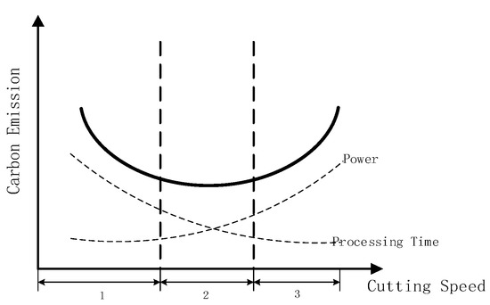
Figure 1.
Cutting speed-carbon emission curve
When the grinding machine power is turned on, the lighting system, operation panel, machine tool frequency converter, servo driver, and other components are turned on. The time is short and the power fluctuation is large, so the start-up energy consumption is ignored. The standby power of the machine P1 consists of the power of the auxiliary system, the motor and the servo power. The time for standby preparation and input of the program before processing is t1. When the Z-axis starts to rotate, the spindle’s no-load rotation power is . No-load standby power is , and no-load standby time is ts. Then the energy consumption Es after the machine is turned on can be expressed as
The empty cutting energy consumption of the cylindrical grinding machine includes the movement of the X-axis of the head frame and the movement of the Z-axis of the grinding wheel. The X-axis rotation and the Z-axis movement power are respectively , . Therefore, the energy consumption of air cut can be expressed as
In order to ensure the surface roughness of the parts and avoid the quality problems such as grinding burns, the flow rate and consumption of the cutting fluid change with different grinding wheel linear speeds and table feed speeds, and the wear amount of the grinding wheel also changes, resulting in dynamic changes of the model. For the change of the linear speed of the grinding wheel and the feed rate of the table, the adjustment function is defined as
where , , are the adjustment factors, is the cooling adjustment factor, and is the grinding wheel wear adjustment function. The energy consumption of the auxiliary system includes the energy consumption generated during the cutting time by the power of the filtration and cooling system , and the energy consumption generated during the standby time of the machine tool in the process of loading and unloading parts, so the auxiliary energy consumption of each part processing can be expressed as
Non-cutting process carbon emissions can be expressed as
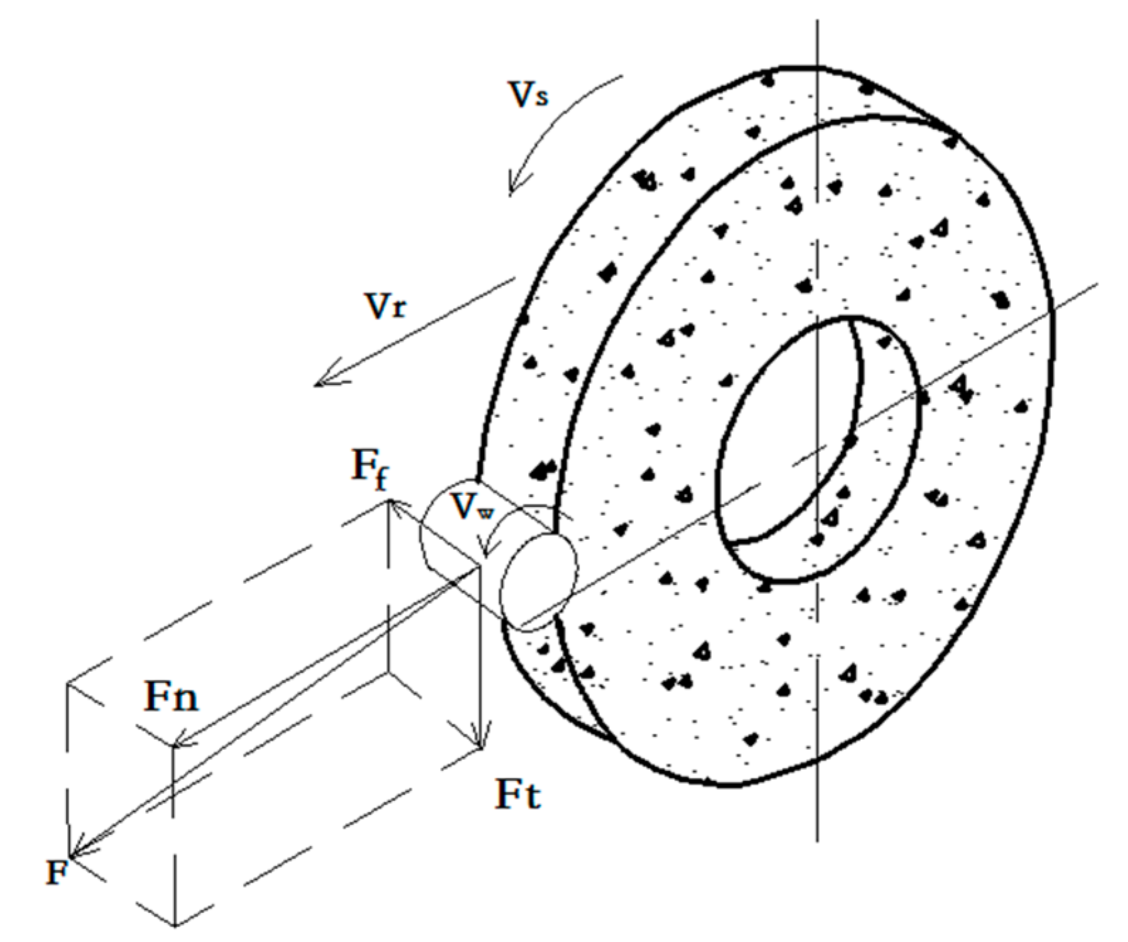
As shown in Figure 2, the grinding force of the grinding wheel is divided into the normal grinding force Fn and the tangential grinding force Ft. The machining power of the grinding Pm is mainly determined by the tangential grinding force and the linear velocity.
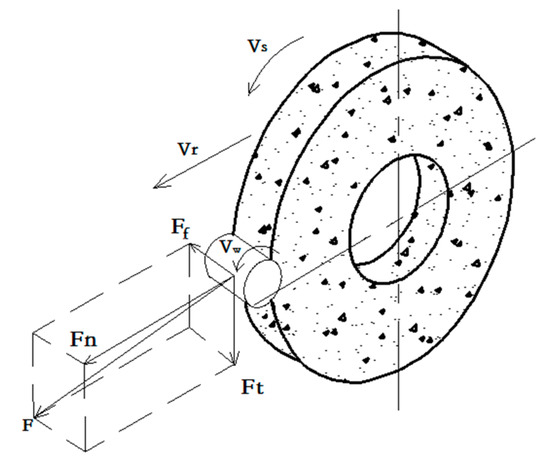
Figure 2.
Grinding wheel force analysis
The speed of the wheel is recorded as follows:
where d0 is the diameter of the grinding wheel, and n0 is the grinding wheel speed.
The tangential grinding force is an important parameter for power calculation. The index in the empirical formula is calculated by experimental data to obtain the actual tangential force of this kind of grinding wheel. The mathematical formula of the cylindrical grinding force is , and is an experimental variable based on different processing environments. The experimental value of the grinding force of the grinding wheel is taken as the natural logarithm, and the regression equation is shown as follows:
The data of grinding consumption obtained in the experiment were coded, the large value is +1, the small value is −1, and the four coefficients b0, b1, b2, and b3, of the regression equation are calculated according to the data of the grinding force. In the grinding, is the i-th grinding variable, is the grinding wheel linear speed , is the grinding wheel cutting feed amount , is the workpiece rotation speed, and is the j-th experimental value of the i-th grinding amount. Then find the three values in the regression equation:
Assuming that ,, then . Substitute it for in the regression equation.
Substitute b0, b1, b2, and b3 with their values in Equation (14) to calculate the Ft, and the actual tangential force is determined according to different depths of cut, wheel speeds, and table feed speeds. The processing energy consumption model takes the form of integral, and the power from 0 to tm is integrated to obtain the energy consumption value. The Em expression of grinding energy consumption is
Then total carbon emissions from the grinding process are
2.3. Cost Model in the Grinding Process
The processing cost of a single part increases with the increase of processing time. The grinding cost is mainly divided into two aspects: processing cost and loss cost. With the part affected by the optimization variable taken into consideration, the grinding process cost model is established. The processing cost includes standby, empty cutting, energy consumption cost of cutting operation, the labor cost during processing time and the use cost of auxiliary equipment, and thus the processing cost expression for each process is shown as follows:
where Cm is the grinding cost (yuan), Me is the electricity cost (yuan/s), and Mas is the labor cost and the use cost of auxiliary equipment (yuan/s); tair is the empty cut time (s); ap is the depth of cut (m) at which the grinding load is generated and it can be known based on processing requirements; the number of processing batches is Q.
Loss costs include wheel loss and cutting fluid consumption, and multiple wheel dressings are required during machining of the part until the wheel is reduced to the minimum diameter. The cost of the grinding wheel Closs is
where Ma is the grinding wheel cost (yuan/mm3); is the wheel width; r is the workpiece radius; G is the grinding ratio.
The consumption of cutting fluid consists of the portion of the machined surface that rises in temperature and evaporates into the air, the portion taken away by the chip, and the portion deposited on the surface of the part. Cutting fluid consumption cost Club (yuan) is
where Ml is the unit cost of cutting fluid consumption (yuan/L); llub is the cutting fluid flow rate (L/s).
The total cost of grinding is
2.4. Constraint and Optimization Model
With the grinding speed constrained, the grinding wheel speed vs must meet the following requirement:
where nmin and nmax represent the minimum and maximum speeds of the CNC grinding machine spindle, respectively.
The tangential feed amount vr of the grinding wheel needs to be within the range of the maximum and minimum values of the spindle feed of the machine tool, that is
The workpiece rotation speed vw needs to be within the range of the maximum and minimum values of the workpiece speed of the CNC grinding machine, that is
With the cutting force constrained, the grinding wheel’s tangential force needs to be less than the maximum cutting force to protect the grinding wheel and the surface quality of the part, namely
Power constraint, the calculated power needs to be less than the maximum power of the CNC grinding machine, namely
The surface quality of the machine is constrained. The surface roughness value needs to be greater than the minimum machining roughness value of the machine tool. It is also an important condition for restraining the linear speed vs of the grinding wheel and the feed rate vw of the table. According to the Ono theory [41], the surface roughness expression of the external grinding is
where is the cutting edge spacing considered by volume density; is half of the cutting edge angle; is the wheel diameter.
In summary, the low-carbon and low-cost parameter multi-objective optimization model in the grinding process is
3. Parameter Optimization Based on Improved NSGA-II Algorithm
3.1. Improved NSGA-II Algorithm
To solve the multi-objective optimization problems, the weighted summation method is used to assign weights to each target value, and the multi-objective problem is simplified to a single-objective problem. However, there is no standard for the assignment of target weights, and the objective functions usually have different dimensions. If the weight value cannot be determined between the carbon emissions and the cost cash, such as in this paper, it will have a greater impact on the calculation results. The algorithm used by a multi-objective function in the MATLAB program is an improved multi-objective optimization algorithm based on the non-dominated sorting genetic algorithm (NSGA-II) with an elite strategy, which can effectively solve the multi-objective optimization problem.
The characteristics of the genetic algorithm include determining the dominance and non-inferiority of the individual, and comparing and judging the better target individual. Based on the dominating judgment order value, the individuals in the population are assigned to different front-ends according to the size, and the higher the front, the stronger the dominance. The crowding distance is used to calculate the distance between a certain body in a front-end and other individuals in the front-end, and to characterize the degree of crowding between individuals—the greater the distance, the better the diversity of the population. The improved algorithm introduces the optimal front-end individual coefficients unique to the gamultiobj function, defines the proportion of individuals in the optimal front-end in the population, and also directly determines the number of individuals retained during the pruning process.
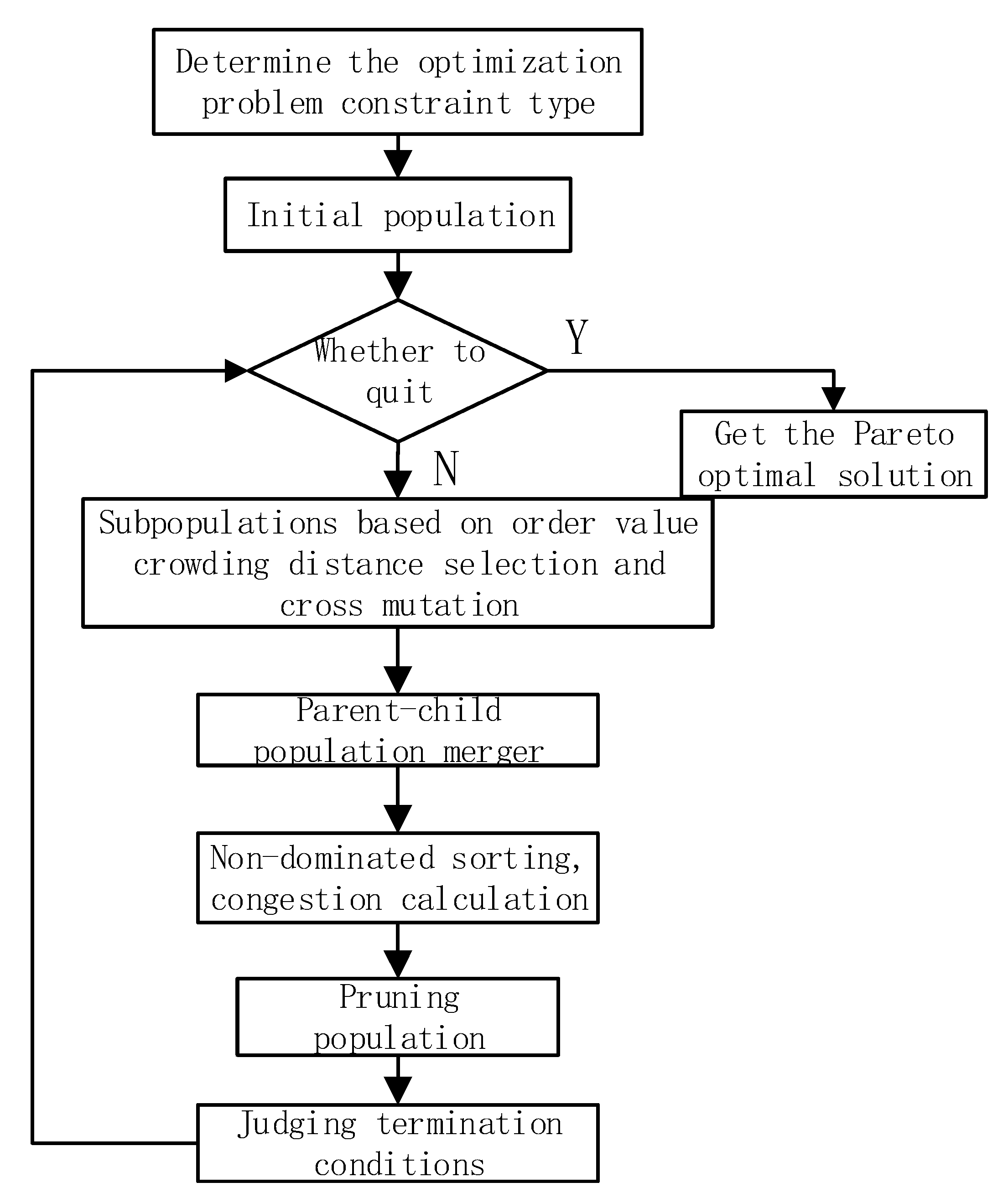
The algorithm flow is to first determine the constraint type of the optimization problem, generate the initial population, and judge whether the algorithm can be exited. And if it exits, get the Pareto optimal solution. If not, the population will evolve into the next generation. In the process of evolution, the gamultiobj function only uses the tournament selection method based on the order value and the crowded distance. The selected individual is assigned to several front-ends to generate the parent population. The parent population crosses, and the mutation produces the children. The gamultiobj function allows the elite to automatically retain, and the scaling function is no longer needed. The parent and the child are merged, and the individuals in the population are sorted by the non-dominated sorting function so that all the merged individuals are assigned to different front-ends. Then the crowded distance is used to calculate the distance between each body in a front-end and its neighbors. According to the optimal front-end individual coefficient, individuals equal to the size of the population are pruned in the population twice as large as the parent–child mergence to obtain a new parent population, and it is judged whether the iteration is terminated or whether the algorithm can be exited. The algorithm flow is shown in Figure 3.
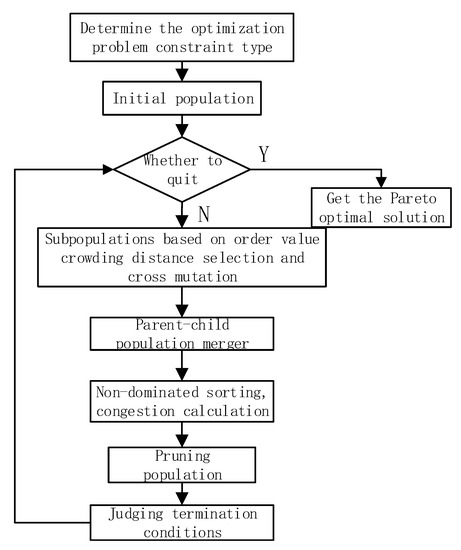
Figure 3.
Algorithm flow chart.
3.2. Optimization Target Solving
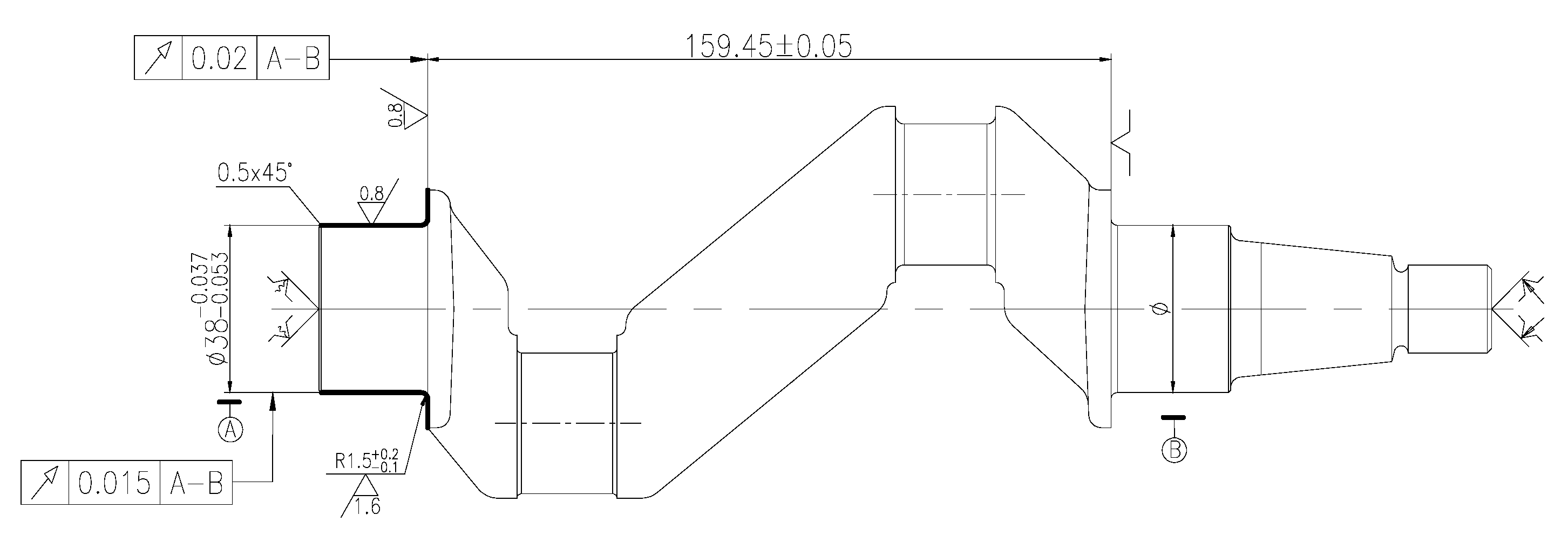
The air compressor crankshaft blank of 45# steel was selected, and the second main journal of the crankshaft is finely ground by a face cylindrical grinding machine, M-181. The diameter of the main journal is φ 37.96–37.944, the root radius is R 1.4–1.7, the outer diameter of the main shaft is 0.015, and the roughness of the outer circle is Ra 0.8. The process drawing is shown in Figure 4, and the actual processing is shown in Figure 5. The grinding machine uses a 100# resin-bonded diamond grinding wheel to grind the outer end surface of the shaft parts, and the grinding precision and smoothness are high; the longitudinal movement of the grinding wheel frame is driven by the gear oil pump, and the movement is stable to ensure the uniform feeding speed of the grinding wheel; double-paired high-precision rolling bearings can make high rotation accuracy and rigidity. The relevant parameters of the machine tool are shown in Table 1.
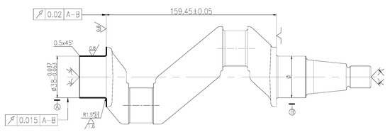
Figure 4.
Fine-grinding the second main journal of the crankshaft.

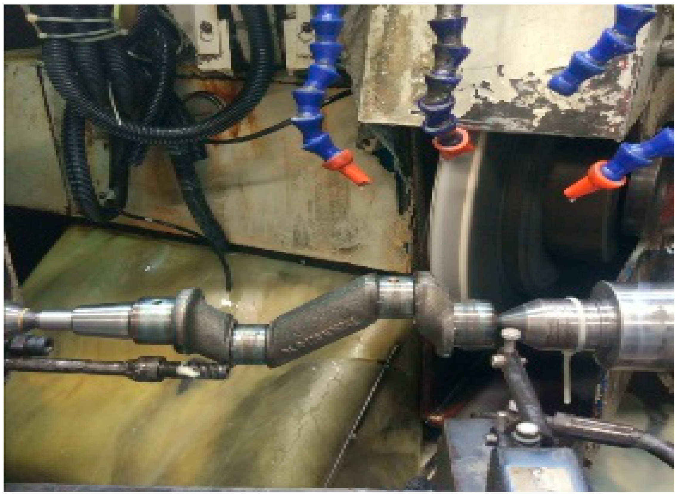
Figure 5.
Actual machining of the crankshaft.

Table 1.
CNC cylindrical grinding machine parameters.
Control the grinding machine standby, air cutting, and other stages of operation. At each stage, use the three-phase four-wire wiring method to lap the power recorder and collect the power value of each stage of the machine tool. At the same time, the current-monitoring equipment is used to monitor the data reliability of the power meter. Finally, when the second main journal of the crankshaft is ground, a top force-measuring instrument is installed to detect and collect the grinding force at different cutting speeds in real-time. The experiment for the grinding force is carried out to obtain the parameters in Table 2, and the parameters are introduced into the model of the second part. The specific experimental instruments are shown in Figure 6 and Figure 7, and the corresponding parameter values are shown in Table 3.
Table 2.
Grinding force experiment.
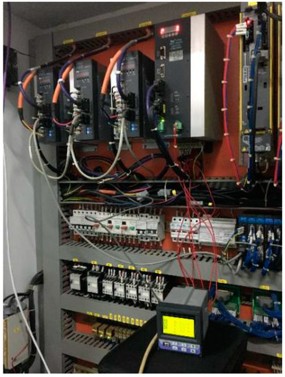
Figure 6.
Grinding machine power recorder.
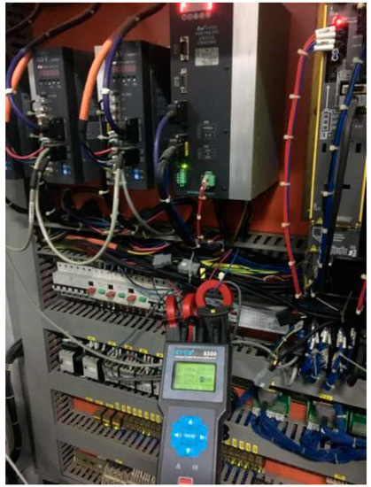
Figure 7.
Grinding machine current monitor.
Table 3.
Grinding parameters.
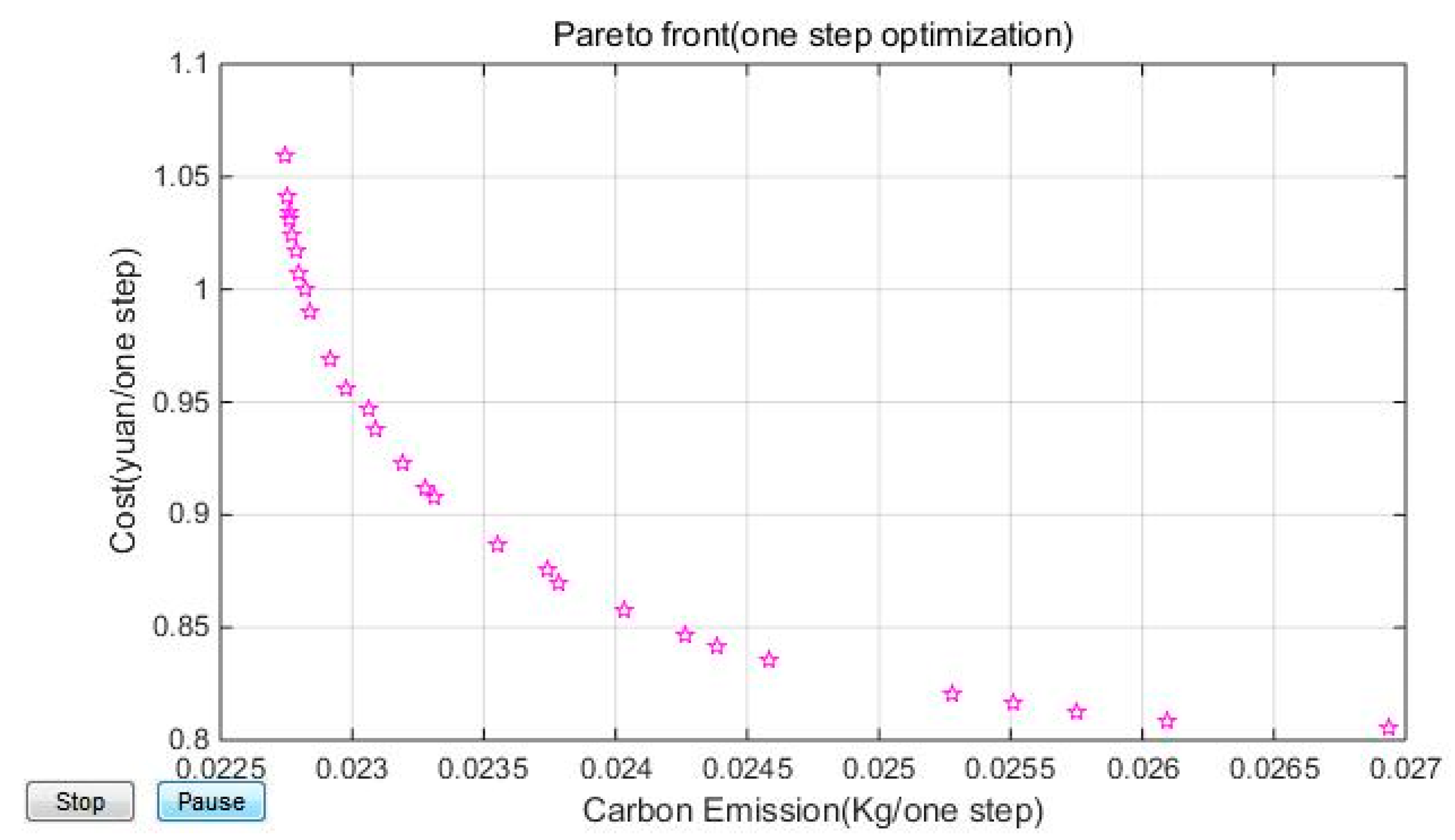
Set the optimal front-end individual coefficient to 0.3, the population size to 100, the maximum evolutionary algebra to 300, the stop algebra to 300, and the fitness function deviation to 0.001 to calculate the results. Since the initial population of the algorithm is randomly generated, the operation results obtained each time are different. The Pareto front-end values obtained from the result of a certain operation is shown in Figure 8. Table 4 shows the specific parameters of the 30 optimal front individuals, each row representing an individual speed of the grinding wheel outer circle, the cutting feed rate, the rotational speed of the workpiece, the individual’s carbon emissions, and costs.
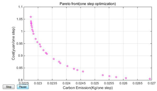
Figure 8.
First front-end individual distribution map.
Table 4.
Pareto front-end values obtained from a certain operation.
3.3. Fuzzy Matter Element-Based Decision-Making
Multi-objective decision-making schemes include use things, features, and fuzzy magnitudes to quantitatively analyze and calculate things. Assume that the thing is the plan , and the feature is the evaluation index (for the purposes of this paper, the evaluation index is the wheel speed, the table feed speed, the carbon emission, and the cost), and the fuzzy value gives the value of , thereby constituting the matter element. For the optimization model of this paper, take the smaller and better decision, and the metric is determined by the correlation coefficient .
According to the scheme, the characteristics and the correlation coefficient, it can construct the complex fuzzy matter element of the dimension correlation coefficient of a thing.
Rw is the weighted composite element for each decision-making indicator, and the weight of the i-th evaluation indicator for each scenario is .
The weighted average centralized processing is used to construct the correlation fuzzy matter element, namely
The minimum value is obtained by sorting the degree of association, and the optimal solution is K21. The results in the single target case are obtained and compared, as shown in Table 5.
Table 5.
Comparison of optimization results.
The best variable for the second main spindle refining of the crankshaft with low carbon and low cost is the grinding wheel linear velocity of 24.235 m/s, the spindle feed speed is 0.00016 m/s, the workpiece rotation speed is 14.0428 m/s, and the carbon emission is 0.0252 kg/piece. The processing cost is 0.825 yuan/piece. With low carbon as the goal, the grinding wheel’s linear speed is high, the processing time is short, but the grinding wheel wear and cutting fluid usage are significant and the cost is high; With low cost as the target, the low linear speed of the grinding wheel reduces the amount of wear and the amount of cutting fluid, but the processing time is long and the carbon emission is high.
4. Conclusions
This paper systematically analyzes the energy consumption characteristics and parts-manufacturing costs of various stages of machine tools in grinding. An optimization model for the external grinding parameters with the minimum carbon emission and the optimal cost as the multi-objective is established. The use of auxiliary tools and the division of the whole process are considered in the modeling process. Considering the dynamic change of cutting fluid and the service life of the grinding wheel, an adjustment function is introduced based on the linear speed of the grinding wheel and the feed rate of the working table. The optimized grinding parameters are calculated by using the NSGA-II algorithm, and these parameters are evaluated through the fuzzy matter-element decision method. The machining process is fitted in a single grinding depth during the modeling process, but during the actual production, one part often requires multiple-time grinding. According to different grinding depth and surface roughness values, applying them in the multi-objective optimization dynamic model can realize step-by-step optimization in machining and be referred to for the selection of grinding process parameters.
Author Contributions
Conceptualisation, M.H. and Q.G.; Investigation and experiment, Y.S., S.T. and Y.W.; Visualisation, writing—review and editing, Y.S., M.H. and Q.G. All authors have read and agreed to the published version of the manuscript.
Funding
This research received no external funding.
Acknowledgments
The work described in this paper was supported by the 58th postdoctoral science foundation program of China (Grant No. 2015M581301), the National Natural Science Foundation of China (Grant No. 51775392 and 51675388), the Educational Commission of Hubei Province (Grant No. B2018069), the National Science Foundation of Hubei province (Grant No. 2019CFB384), and the Key Laboratory of Automotive Power Train and Electronics (Grant No. ZDK1201802). These financial contributions are gratefully acknowledged.
Conflicts of Interest
The authors declare no conflict of interest.
References
- Priarone, P.C. Quality-conscious optimization of energy consumption in a grinding process applying sustainability indicators. Int. J. Adv. Manuf. Technol. 2016, 86, 2107–2117. [Google Scholar]
- Arriandiaga, A.; Portillo, E.; Sánchez, J. A new approach for dynamic modelling of energy consumption in the grinding process using recurrent neural networks. J. Neural Comput. Appl. 2016, 27, 1577–1592. [Google Scholar]
- Salonitis, K. Energy efficiency assessment of grinding strategy. Int. J. Energy Sect. Manag. 2015, 9, 20–37. [Google Scholar] [CrossRef]
- Jiang, P.; Li, G.L.; Liu, P.X.; Jiang, L.; Li, X.Z. Energy consumption model and energy efficiency evaluation for CNC continuous generating grinding machine tools. Int. J. Sustain. Eng. 2017, 10, 226–232. [Google Scholar] [CrossRef]
- Lv, J.; Peng, T.; Tang, R. Energy Modeling and a Method for Reducing Energy Loss Due to Cutting Load During Machining Operations. J. Proc. Inst. Mech. Eng. Part B J. Eng. Manuf. 2019, 233, 699–710. [Google Scholar] [CrossRef]
- Calleja, A.; Bo, P.; González, H.; Bartoň, M.; de López Lacalle, L.N. Highly-accurate 5-axis flank CNC machining with conical tools. Int. J. Adv. Manuf. Technol. 2018, 97, 1605–1615. [Google Scholar]
- Draganescu, F.; Gheorghe, M.; Doicin, C. Models of Machine Tool Efficiency and Specific Consumed Energy. J. Mater. Process. Technol. 2003, 141, 9–15. [Google Scholar] [CrossRef]
- Aramcharoen, A.; Mativenga, P.T. Critical factors in energy demand modelling for CNC milling and impact of toolpath strategy. J. Clean. Prod. 2014, 78, 63–74. [Google Scholar] [CrossRef]
- Gutowski, T.; Dahmus, J.; Thiriez, A. Electrical energy requirements for manufacturing processes. In 13th CIRP International Conference on Life Cycle Engineering; CIRP International Leuven: Leuven, Belgium, 2006. [Google Scholar]
- Liu, F.; Wang, Q.; Liu, G. Content Architecture and Future Trends of Energy Efficiency Research on Machining Systems. J. Mech. Eng. 2013, 49, 87. [Google Scholar] [CrossRef]
- Shin, S.J.; Woo, J.; Rachuri, S. Energy efficiency of milling machining: Component modeling and online optimization of cutting parameters. J. Clean. Prod. 2017, 161, 12–29. [Google Scholar] [CrossRef]
- Liu, F.; Liu, P.J.; Li, C.B.; Tuo, J.B.; Cai, W. The Statue and Difficult Problems of Research on Energy Efficiency of Manufacturing Systems. J. Mech. Eng. 2017, 53, 1–11. [Google Scholar] [CrossRef]
- Park, C.-W.; Kwon, K.-S.; Kim, W.-B.; Min, B.-K.; Park, S.-J.; Sung, I.-H.; Yoon, Y.-S.; Lee, K.-S.; Lee, J.-H.; Seok, J. Energy consumption reduction technology in manufacturing—A selective review of policies, standards, and research. Int. J. Precis. Eng. Manuf. 2009, 10, 151–173. [Google Scholar] [CrossRef]
- Trianni, A.; Cagno, E.; Farné, S. Barriers drivers and decision making process for indus-trial energy efficiency: A broad study among manufacturing small and medium-sized enterprises. J. Appl. Energy 2016, 162, 1537–1551. [Google Scholar] [CrossRef]
- Abdelaziz, E.A.; Saidur, R.; Mekhilef, S. A review on energy saving strategies in industrial sector. J. Renew. Sustain. Energy Rev. 2011, 15, 150–168. [Google Scholar] [CrossRef]
- Dietmair, A.; Alexander, V. A Generic Energy Consumption Model for Decision Making and Energy Efficiency Optimisation in Manufacturing. Int. J. Sustain. Eng. 2009, 2, 123–133. [Google Scholar] [CrossRef]
- Cai, W.; Liu, C.; Zhang, C.; Ma, M.; Rao, W.; Li, W.; He, K.; Gao, M. Developing the ecological compensation criterion of industrial solid waste based on emergy for sustainable development. J. Energy 2018, 157, 940–948. [Google Scholar] [CrossRef]
- Cai, W.; Liu, F.; Zhou, X.; Xie, J. Fine energy consumption allowance of workpieces in the mechanical manufacturing industry. J. Energy 2016, 114, 623–633. [Google Scholar] [CrossRef]
- Greinacher, S.; Lanza, G. Optimisation of lean and green strategy deployment in manufacturing systems. J. Appl. Mech. Mater. 2015, 794, 748–785. [Google Scholar] [CrossRef]
- Cai, W.; Liu, C.; Lai, K.-H.; Li, L.; Cunha, J.; Hu, L. Energy performance certification in mechanical manufacturing industry: A review and analysis. J. Energy Convers. Manag. 2019, 186, 415–432. [Google Scholar] [CrossRef]
- Ma, F.; Zhang, H.; Hon, K.; Gong, Q.S. An optimization approach of selective laser sintering considering energy consumption and material cost. J. Clean. Prod. 2018, 199, 529–537. [Google Scholar] [CrossRef]
- Jiang, Z.; Ding, Z.; Liu, Y.; Wang, Y.; Hu, X.; Yang, Y. A data-driven based decomposition–integration method for remanufacturing cost prediction of end-of-life products. Robot. J. Comput. Integr. Manuf. 2020, 61, 101838. [Google Scholar] [CrossRef]
- Lin, W.; Yu, D.; Wang, S.; Zhang, C.; Zhang, S.; Tian, H.; Luo, M.; Liu, S. Multi-objective teaching–learning-based optimization algorithm for reducing carbon emissions and operation time in turning operations. J. Eng. Optim. 2015, 47, 994–1007. [Google Scholar] [CrossRef]
- Wei, Y.; Hua, Z.; Zhi-gang, J.; Hon, K.K.B. A new multi-source and dynamic energy modeling method for machine tools. Int. J. Adv. Manuf. Technol. 2018, 95, 4485–4495. [Google Scholar] [CrossRef]
- Bustillo, A.; Urbikain, G.; Perez, J.M.; Pereira, O.M.; Lopez de Lacalle, L.N. Smart optimization of a friction-drilling process based on boosting ensembles. J. Manuf. Syst. 2018, 48, 108–121. [Google Scholar] [CrossRef]
- Shen, N.Y.; Wang, W.D.; Li, J.; Cao, Y.L.; Wang, Y. Modelling and Analysis of Grinding Energy Consumption in Non-circular Grinding Process. J. Mech. Eng. 2017, 53, 208–216. [Google Scholar] [CrossRef]
- Li, H.N.; Yu, T.B.; Wang, Z.X.; Zhu, L.D.; Wang, W.S. Detailed modeling of cutting forces in grinding process considering variable stages of grain-workpiece micro interactions. Int. J. Mech. Sci. 2016, 126, 319–339. [Google Scholar] [CrossRef]
- Zhang, Y.B.; Li, C.H.; Ji, H.J. Analysis of grinding mechanics and improved predictive force model based on material-removal and plastic-stacking mechanisms. Int. J. Mach. Tools Manuf. 2017, 122, 67–83. [Google Scholar] [CrossRef]
- Liu, P.J.; Junbo, T.; Liu, F.; Li, C.B.; Zhang, X.C. A Novel Method for Energy Efficiency Evaluation to Support Efficient Machine Tool Selection. J. Clean. Prod. 2018, 191, 57–66. [Google Scholar] [CrossRef]
- Paetzold, J.; Kolouch, M.; Wittstock, V.; Putz, M. Methodology for process-independent energetic assessment of machine tools. J. Procedia Manuf. 2017, 8, 254–261. [Google Scholar] [CrossRef]
- Jiang, Z.; Ding, Z.; Zhang, H.; Cai, W.; Liu, Y. Data-driven ecological performance evaluation for remanufacturing process. J. Energy Convers. Manag. 2019, 198, 111844. [Google Scholar] [CrossRef]
- Ding, Z.; Jiang, Z.; Zhang, H.; Cai, W.; Liu, Y. An integrated decision-making method for selecting machine tool guideways considering remanufacturability. Int. J. Comput. Integr. Manuf. 2018, 1–12. [Google Scholar] [CrossRef]
- Schudeleit, T.; Züst, S.; Wegener, K. Methods for evaluation of energy efficiency of machine tools. J. Energy 2015, 93, 1964–1970. [Google Scholar] [CrossRef]
- Ma, F.; Zhang, H.; Gong, Q.S.; Hong, K.K.B. A Novel Energy Evaluation Approach of Machining Processes Based on Data Analysis. J. Energy Sources Part A Recovery Util. Environ. Eff. 2019, 1–15. [Google Scholar] [CrossRef]
- Cai, W.; Lai, K.; Liu, C.; Wei, F.F.; Ma, M.D.; Jia, S.; Jiang, Z.G.; Lv, L. Promoting sustainability of manufacturing industry through the lean energy-saving and emission-reduction strategy. J. Sci. Total Environ. 2019, 665, 23–32. [Google Scholar] [CrossRef]
- Jia, S.; Yuan, Q.; Cai, W.; Li, M.; Li, Z. Energy modeling method of machine-operator system for sustainable machining. J. Energy Convers. Manag. 2018, 172, 265–276. [Google Scholar] [CrossRef]
- Liu, Z.; Wang, S.; Wan, J.; Liu, G. Green Product Assessment Method Based on Fuzzy-Matter Element. J. China Mech. Eng. 2007, 18, 166–170. [Google Scholar]
- Wang, Y.; Zhang, H.; Zhang, Z.; Wang, J. Development of an Evaluating Method for Carbon Emissions of Manufacturing Process Plans. J. Discret. Dyn. Nat. Soc. 2015, 2015. [Google Scholar] [CrossRef]
- Zhang, L.; Ma, J.; Fu, Y.G. Carbon Emission Analysis for Product Assembly Process. J. Mech. Eng. 2016, 52, 151–160. [Google Scholar] [CrossRef]
- Li, C.; Cui, L.; Liu, F.; Li, L. Multi-objective NC Machining Parameters Optimization Model for High Efficiency and Low Carbon. J. Mech. Eng. 2013, 49, 87–96. [Google Scholar] [CrossRef]
- Zhuang, S.X. Grinding Technology; Mechanical Industry Press: Beijing, China, 2007; pp. 53–55. [Google Scholar]


© 2019 by the authors. Licensee MDPI, Basel, Switzerland. This article is an open access article distributed under the terms and conditions of the Creative Commons Attribution (CC BY) license (http://creativecommons.org/licenses/by/4.0/).