Abstract
The performance of cross-flow ultrafiltration is greatly influenced by permeate flux behavior, which depends on many factors, including solution properties, membrane characteristics, and operating conditions. Currently, most research focuses on improving membrane performance, both in terms of permeability and selectivity. Only a few studies have paid attention to how the membrane module is configured and operated. In this study, the geometric design and operating conditions of a membrane module are considered as multivariable optimization variables. The objective function is the annual cost. The cost consists of a capital investment depending on the plant scale and an operating expense associated with energy consumption. In the optimization problem, the channel dimensions (width × length × height), and operating conditions (the inlet pressure and recirculation flow rate) were considered as decision variables. The operating configuration of the membrane plant is assumed to be feed and bleed mode, and a model including the pressure drop is introduced. The model is used to simulate the membrane plant and calculate the membrane area and energy usage, which are directly related to the total cost. The genetic algorithm is used for the optimization. The effect of individual parameters on the total cost is discussed.
1. Introduction
The performance of cross-flow ultrafiltration is greatly influenced by the behavior of permeate flux. The flux declination depends on many factors, including solution properties, membrane characteristics, and operating conditions. Currently, most research has focused on improving membrane performance in terms of permeability and selectivity [1,2]. Only a few studies have paid attention to how the membrane module is configured and operated [3].
The selection of a specific membrane module geometry for a specific application is affected by several factors: the fabrication method, energy consumption, and the possibility of fouling [4]. Manufacturers usually suggest the geometric design of the membrane module from the fabrication aspect [4]. There is little evidence that energy efficiency is primarily considered in their approach. Presently, with an increase in energy costs and a decrease in membrane price, energy efficiency should be given greater emphasis in the design of membrane module geometry. Therefore, a module design methodology which includes energy consideration is necessary.
In addition, the determination of operating conditions is normally derived from experience, obtained from the handbook or by recommendation from the membrane manufacturer. However, the performance of the membrane system, which is governed by the permeate flux equation, varies considerably between different situations and applications. In this manner, a general methodology for the design and operation scheme should be studied for any specific application.
In our earlier work [5], a simple combined model, which simultaneously considers pore blockage and cake filtration, was proposed and proved its potential for estimation of flux decline in cross-flow ultrafiltration of protein solution. In our other study [6], the steady-state permeate flux was predicted and correlated to operating conditions from the model. The methodology can be generalized for any particular process to determine the steady state operation equations of the membrane for protein separation. From the operation equation, an optimal design for any certain application can be obtained. This design is dependent on various factors, such as plant capacity, desired recovery, and the energy cost at the specific location. The optimal design will give additional information for supporting the assessment of existing membrane modules and the fabrication and operation decisions of the new membrane system.
However, there are few studies on the optimization of membrane processes and cost estimation. For example, in the study of Wiley, Fell, and Fane [4], membrane module design for brackish water desalination was optimized. However, the configuration is single-pass operation, and the cost only included the membrane cost and energy cost. In the study of Sethi and Wiesner [7], a cost model for the removal of natural organic matter was developed, but the optimization was not conducted. In membrane technology, the feed and bleed configuration, which merges the batch and the single-pass operations, is widely used for continuous full-scale operation [8,9]. In our previous study [10], a simulation and optimization model of a feed and bleed membrane system was investigated. The model was solved by a simple discretization method, and some discontinuous points of the objective function appeared. Moreover, the fixed cost was assumed independently of the system size. Therefore, in this study, the optimization of a membrane module for protein ultrafiltration is considered, in which the geometric design and operating conditions are variables. A system of ordinary differential equations is developed and numerically solved to improve the accuracy of the model. The objective function is the annual cost. The cost consists of various types of capital investments depending on the plant scale and an operating expense associated with energy consumption. The core facilities of the membrane plant are classified into pumps, valves and pipes, instruments and controls, vessels and frames, and miscellaneous. The cost of each category is individually correlated to plant scale, specifically the membrane area. A model incorporating the pressure loss is introduced to simulate the membrane plant and calculate the membrane area and energy usage, which are directly related to the total cost. In the optimization problem, the channel dimensions (width × length × height) and operating conditions (the inlet pressure and recirculation flow rate) were considered as decision variables.
Among various optimization techniques, evolutionary algorithms which are a broad class of population-based metaheuristic optimization techniques inspired by the evolution of species in nature, have been effectively utilized in different fields to solve numerous optimization problems [11]. Evolutionary algorithms, including the genetic algorithm, have some advantages such as being derivative-free and having durable robustness, flexibility, and the ability to discover the global optimum. Therefore, the genetic algorithm is used in this study to find the most cost-effective design and operation of the membrane module.
2. Process Configuration and Model Calculation
In this section, the configuration of the plant operation is introduced. The system of ordinary differential equations for modeling the membrane plant is developed. The results from the simulation are essential for the estimation of the membrane area and energy usage, which are two significant factors affecting the total cost of the plant.
2.1. Membrane Plant Configuration
The operational configuration assumed in developing the model for simulation of membrane plant is presented in this section. The plant’s operation is supposed to be a continuous feed and bleed mode, as shown schematically in Figure 1. A summary of the notations is presented in Table 1. There are two important pumps in this configuration: the feed pump supplies the appropriate transmembrane pressure, while the recirculation pump supports the required cross-flow rate through the modules. At startup, the feed pump is used to fill the recirculation/module loop, and then the recirculation pump is started. After the system is stabilized, a small fraction of the flow is continually withdrawn as concentrate at a flow rate (R).
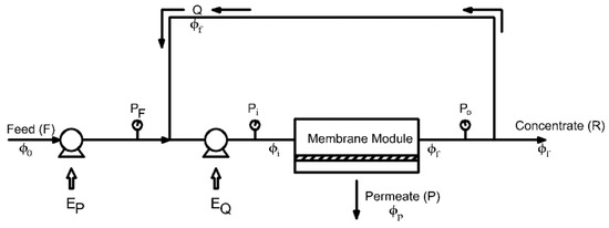
Figure 1.
Schematic configuration of feed-and-bleed mode membrane system.

Table 1.
Summary of system configuration notations.
2.2. Modeling of Membrane Modules
In ultrafiltration, the pressure is also a significant factor affecting the flux behavior; therefore, the friction loss should be taken into consideration. The model proposed in this study is the improvement of our previous work [10]. In [10], rather than using incremental length step, the channel is subdivided into a number of segments by the protein concentration from the inlet (ϕi) to the outlet (ϕf). The concentration of the protein solution is expressed as a volume fraction. For each control volume, the transport properties, the permeate flux equation in [6], and friction loss formulae are applied. Then, the length of each increment and the pressure of the next segment can be obtained by mass balance. However, the results show that there are some discontinuous points due to discretization. Therefore, in this study, the chain rule of differentiation [12] is applied and a system of ordinary differential equations was developed. The derivatives are taken with respect to the concentration instead of the length. The mathematical form is discussed in detail as follows.
The overall mass balance and component material balance give:
Material balance around the mixing junction of the feed and recirculation stream provides:
In Karasu’s study [13], the author reconstituted various solutions with different protein concentrations from the whey protein concentrated powder (ALACENTM, acquired from NZMP Ltd.) and measured their rheological properties. Therefore, the correlation equations from [13] can be used to estimate the properties of protein solution in the simulation.
The correlation equation for the viscosity of protein solution is:
in which μm, ϕm are the viscosity and concentration of the mixture (solution), respectively.
The density of protein solution (ρm) can be approximated from the density of water (1000 kg/m3) and the density of dry protein powder (1360 kg/m3)
The permeate flux through the membrane is (obtained from [6])
in which P is the transmembrane pressure, u is the cross-flow velocity, and dh is the hydraulic diameter of the flow channel.
From the shear-induced diffusion or surface transport model, the permeate flux depends linearly on the membrane shear rate [14]. The increase of module height will decrease the shear rate at the membrane surface. In the experiment of this study, the height of the module channel remained constant. Therefore, in order to extend the application of the permeate flux equation to other systems which has different module heights, the correction factor dh0/dh should be introduced as follows.
where dh0 is the value of hydraulic diameter of the membrane module used in the study [5].
The equation for permeate flux can be rewritten as:
or in terms of shear rate at the membrane surface , where h is the channel height:
The flow rate and cross-flow velocity at the entrance of the membrane module
where w × h is the cross-sectional area of the flow channel, w is the width, and h is the height of the membrane module.
The flow rate and velocity change along the length of the membrane module are determined by the mass balance with the assumption that there is no protein in the permeation, as:
After applying the product rule and then rearranging, we obtain
The mass balance for the element control volume along the length of the membrane:
Incorporating with Equation (13), the differential equation for the length can be obtained:
The pressure loss is calculated by the Darcy–Weisbach equation in differential form as follows
in which f is the friction factor
- for laminar flow in a rectangular channel (Re < 2000) [15].
- for turbulent flow (Re > 2000) (smooth pipes, Blasius correlation [16]).
Incorporating with Equation (16), the differential equation for the pressure can be obtained:
Finally, the system of ordinary equations for the membrane module system was developed as follows.
In the interval [ϕi, ϕf] and the initial condition
The system of the ordinary equations can be solved by the Runge–Kutta 4th order method [17]. The solution is the flow rate, the length, and the pressure at the final concentration. After the total length was determined, the membrane area was obtained:
The total energy generated by the pumps:
In this equation,
- EP, EQ are the power supplied by the feed pump and recirculation pump, respectively
- PF, Pi, Po are the pressure at the outlet of the feed pump, at the inlet and outlet of the membrane module, respectively
- ΔPdrop is the pressure drop in the membrane module
For desirable feed flow rate, recirculation flow rate, and initial and final concentration, the total membrane area and energy usage are calculated from the simulation model with the governing equation of permeate flux. The total membrane area and energy usage are the important factors in the estimation of the total cost of the filtration plant, and the correlation to the total cost is discussed in the next section.
2.3. Cost Estimation
2.3.1. Operating Cost
The operating cost takes into account the energy expense of the pumps and the cost of membrane replacement. The annual energy expense of the pumps is calculated as
Epumps is the power supplied of the two pumps, feed pump and recirculation pump, and is evaluated by Equation (22). The assumption used in the calculation of annual energy expense is 8000 h/year operation (24 h/day and 333 days/year). η is the efficiency of the pumps, which is set to be 0.7. Energy cost is the electricity price as $/kWh, and is supposed to be 0.08, which is the price for the industrial sector in the United States [18].
The membrane replacement cost is calculated as
where Cmembrane [$/m2/year] is the membrane replacement cost calculated per year and cmembrane [$] is the membrane price per unit area. is the amortization factor, which presents the time value of money [19] and is calculated as a function of interest rate i and the membrane life.
The membrane price is usually about 200 $/m2 [9], and membrane life is 12–18 months. Therefore, the membrane replacement cost per year is roughly estimated as 200 $/m2/year for the interest of I = 8%.
2.3.2. Capital Cost
It is empirically observed that all capital cost components, such as construction cost, pump cost, and equipment cost, are correlated with the plant capacity, size of the main equipment, or other design parameters, in the power-law form [20]:
Instead of directly relating the capital cost of the membrane to capacity, Sethi and Wiesner [7] proposed an approach for predicting capital costs of membrane processes. In this approach, the capital cost is divided into several major categories and the capital cost for each category is developed to improve the accuracy. Membrane system costs generally consist of the costs of pumps and other manufactured equipment. The correlation of each category to the plant capacity is discussed in detail as follows.
Pump Capital Cost
The capital cost for pumps can be estimated using the power-law relation as shown in Equation (25), where the relevant size parameter is the power of the pump:
The cost correlation for general-purpose-single and two-stage-single-suction centrifugal pumps discussed in Perry, et al. [21] was used in this study to calculate the pump capital cost. This relation is as follows:
in which
- I: a cost index ratio for updating the cost to the recent year
- f1: an adjust factor for pump construction material
- f2: an adjust factor for suction pressure range
- L: a factor used to incorporate labor costs
- Q: flow capacity of the pump [m3/h]
- P: pressure outlet of the pump [kPa]
The cost index, I in Equation (27), can be referred to as the chemical engineering (CE) index and obtained from “Chemical Engineering” magazine. The values of CE index of several years were also tabulated in [22]. The cost index I calculated in this study is 2.4 to update the pump cost.
Usually, 40% of the cost is required for labor to install manufactured equipment [23], thus L = 1.4. The factors f1 and f2 can be found in [21]. For the application in food industries, the material was set to stainless steel, indicating that f1 = 1.5. Because the operating pressure of most UF and MF applications are below 10 bar (1 MPa), f2 = 1.0 was used in this study.
In the system configuration used in this study, the size factor (Q × P in Equation (27)) of the two pumps (feed pump and recirculation pump) is calculated as
Capital Cost of Other Equipment
In membrane applications, the membrane area required is the most significant factor which determines the size of the plant [24]. Therefore, the membrane area should be the size parameter used in power-law correlation expression for the estimation of the capital cost of various components.
Sethi [25] segregated nonmembrane equipment and facilities, excluding the pumps which have already been evaluated in Pump Capital Cost, into four main categories: (1) pipes and valves; (2) instruments and controls; (3) tanks and frames; and (4) miscellaneous. The author investigated different sources of data and proposed the calibrated cost correlation for various membrane system components as the following equations:
- Pipes and valves
- Instruments and controls
- Tanks and frames
- Miscellaneous
Annual Capital Cost
The annual capital cost will be obtained from the capital cost based on the amortization factor, as
For the plant design year of 20 years and the interest rate 8%, the amortization factor will be about 0.1.
3. Formulizations of the Problem
3.1. Fix Parameters and Design Variables
The optimization problem is the geometric design and operating condition of the membrane system. The operation is under steady-state conditions. In the design problem, some variables should meet the requirement of the process. These are inlet variables and usually are feed flow F, inlet concentration ϕ0, and outlet concentration ϕf. The protein is assumed to be entirely rejected by the membrane (ϕp = 0).
The decision variables investigated in the optimization problem were: channel geometry (width × length × height), the inlet pressure (Pi), and recirculation flow rate (Q).
3.2. Objective Function
The objective function consists of both capital cost and operating cost expressed per year:
The capital cost includes the cost of membranes, pumps, pipes, and valves, instruments and controls, tanks and frames, miscellaneous (buildings, storage, etc…).
The operating cost includes membrane replacements and pumping energy cost.
3.3. Constraints
The pressure drop should ensure that the pressure at the outlet point will be positive. This constraint is easily set by defining that the objective function is infinity if the outlet pressure is negative.
The bounded constraint also affects the optimization results. Based on typical available data, the physically meaningful ranges, the manufacturing problem, operating properties, etc., the decision variables are usually bounded on a finite range:
where x is the vector of decision variables x = (Pi, Q, w, h), subscript l and u indicate the lower and upper bound.
The system parameters and variables are summarized in Table 2.
Table 2.
System parameters and variables.
3.4. Optimization by Genetic Algorithm
Genetic algorithms (GA), a class of evolutionary algorithms (EA), are adaptive heuristic search algorithms inspired by the evolutionary ideas of natural selection and genetics. The genetic algorithms start with arbitrarily picked parent chromosomes from the search space, each representing a candidate solution, to form an initial population. The fitness of each individual is indicated by the value of the objective function. The population of individual solutions is repeatedly modified in an analogous way to processes happening in nature, such as selection, reproduction by cross-over, and mutation. Over successive generations, the population evolves, and the optimal solution might be achieved by the principles of “survival of the fittest”. More detailed discussions of the genetic algorithm can be found elsewhere, such as in [26].
In this study, the parameters of GA, population size, crossover probability, mutation probability values, were set to be, 100, 1.0, and 0.30, respectively. The selection was based on roulette wheel selection with elitism, which means that the best individual always survives to the next generation. The number of generations was 500. Due to the minimization of the annual total cost, the fitness function was defined as:
4. Results and Discussion
4.1. Effect of Recirculation Flow Rate on the Total Cost
The relationship between the recirculation flow rate and the annual total cost is shown in Figure 2. Other design variables are held constant, inlet pressure TMP = 500 kPa, module height h = 5 mm, module width w = 1 m.
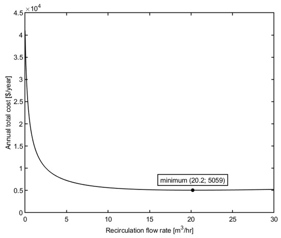
Figure 2.
Effect of recirculation flow rate on the annual total cost of the plant.
As illustrated in the figure, the increase in the recirculation flow rate initially reduces the total cost of the membrane plant. However, further increasing the recirculation flow rate causes the total cost to increase. This might be explained by considering the permeate flux and power consumption. The rise in flow rate leads to an increase in the Reynolds number and the permeate flux, as demonstrated in the Equation (7). Consequently, the required membrane area can be reduced, which results in a decrease in capital investment and membrane replacement cost. Hence, the annual total cost of the plant is minimized. However, from the Equations (17) and (22), it can be obtained that the pressure drop increases rapidly in the turbulent flow regime and faster than the increase in permeate flux (the exponents of the velocity dependency are 1.75 and 1, respectively). The pressure loss is directly related to the power consumption of the pumps or the energy cost. Therefore, as the recirculation flow rate increases, the annual total cost decreases and reaches a minimum value, and then rises again with a further increase in flow rate.
4.2. Effect of Module Inlet Pressure Operation
Figure 3 demonstrates the relation between the operating pressure at the inlet and the annual total cost. Other design variables are held constant, recirculation flow rate Q = 35 m3/h, module height h = 15 mm, module width w = 1 m.
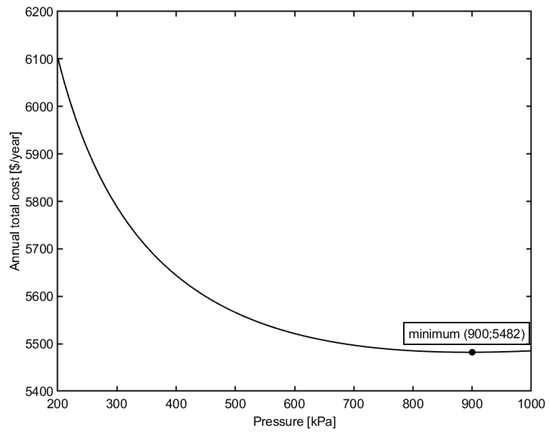
Figure 3.
Effect of inlet pressure on the total cost of the plant.
As illustrated in the figure, the increase in the inlet pressure initially minimizes the annual total cost of the membrane plant. However, a further increase in pressure causes the annual total cost to increase. The explanation is as follows. The permeate flux benefits from the increase in pressure operation with the order of dependence of 0.26, as obtained from Equation (7). Hence, the required membrane area can be reduced, which results in a decrease in the capital investment and membrane replacement cost. Therefore, the annual total cost of the membrane plant is minimized. However, from Equations (22) and (27), it can be obtained that both the power consumption and the initial investment for the pumps rise much faster than the increase of permeate flux (the exponents of the pressure dependency are 1 and 0.4, respectively). Therefore, as the inlet operating pressure increases, the annual total cost decreases and reaches a minimum value, and then rises again with a further increase in operating pressure.
4.3. Effect of Module Height
Figure 4 shows the effect of module height on the total cost. Other design variables are kept constant, inlet pressure TMP = 500 kPa, recirculation flow rate Q = 45 m3/h, module width w = 1 m.
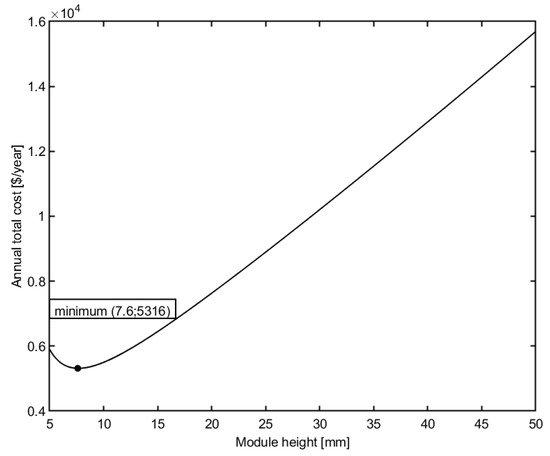
Figure 4.
Effect of module height on the total cost of the plant.
From the figure, it is shown that the decrease in the height of the membrane module will decrease the total cost of the membrane plant. However, a further decrease in module height makes the total cost also increase. The reason is similar to the effect of the recirculation flow rate. The decrease in module height will increase the cross-flow velocity and thus increase the permeate flux. Therefore, the membrane area decreases, which leads to a decrease in the membrane replacement cost. Consequently, the annual total cost of the membrane plant will decrease. However, high velocity affects the pressure loss and hence, energy consumption. Therefore, the annual total cost initially decreases and reaches a minimum value, then rises again with a further decrease in module height.
4.4. Effect of Module Width
Figure 5 shows the effect of module height on the total cost. Other design variables are kept constant, inlet pressure TMP = 500 kPa, recirculation flow rate Q = 35 m3/h, module height h = 10 mm.
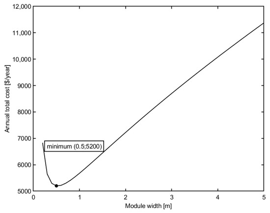
Figure 5.
Effect of module width on the total cost of plant.
Similar to the effect of the recirculation flow rate, it is shown that the decrease in the height of the membrane module will decrease the total cost of the membrane plant. However, a further decrease in module height makes the total cost also increase. The decrease in module width will increase the cross-flow velocity and shear rate, thus increase the permeate flux. Therefore, the membrane area decreases, which leads to a decrease of membrane replacement cost, and the annual total cost of the membrane plant will decrease. However, high velocity affects the pressure loss and hence, energy consumption. Therefore, the annual total cost initially decreases and reaches a minimum value, then rises again with a further decrease in module height.
4.5. Optimum Design
The optimum design of various feed flow rate designs was done in order to illustrate the method. The lower bound for the membrane width is 0.1 m and the lower bound for the module height is 0.5 mm. The results of the design are shown in Table 3.
Table 3.
Optimum design of the membrane module.
From Table 3, it can be obtained that the operating pressure of the optimum design plant is at a high value when the feed flow rate is not so low. When operating at high pressure, the permeate flux increases, resulting a reduction in the membrane area. However, if the operating pressure is too high, it will affect the mechanical stability of the system in addition to the pump cost expression. Therefore, the plant should operate at the maximum allowance of pressure.
Figure 6 shows the total cost per unit flow rate design. The cost per unit flow rate design decreases when the plant size becomes larger. It reflects the economics of scale.
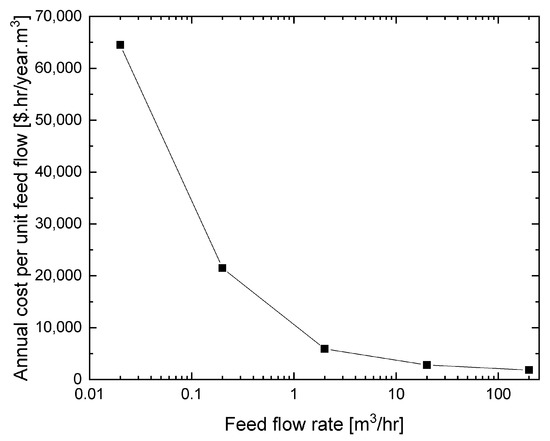
Figure 6.
The behavior of cost per unit flow rate design in optimum condition with plant capacity.
From the results, it can be shown that the membrane plant should be designed as long in channel length but short in channel width to achieve a high cross-flow velocity. The recirculation flow rate is also operated at a moderate value to maintain relatively high cross-flow velocity, but to not consume too much energy for the pump. The channel height should be configured at several millimeters.
From the results it can also be obtained that at different requirements of the process, such as the desired feed flow rate, the membrane plant configuration and operation condition will significantly change. The tendency is difficult to predict. Therefore, the design requirement and permeate flux expression strongly affect the design, selection, and operation strategy in membrane separation processes. There is no general rule, and for a particular system, the permeate flux and the correlation with operating conditions and membrane geometry should be investigated. The design and operating strategy strongly depend on this correlation.
5. Conclusions
In this study, a simulation of a membrane plant was discussed. A system of ordinary differential equations was developed to accurately simulate the membrane module. The system of equations reflects the change of flow properties along the membrane and incorporates the pressure drop. The steady-state permeate flux presented in [6] is assumed as the governing equation for the filtration process. An economic model including the capital cost as well as the operating cost was used to evaluate the performance of the membrane plant. The effect of operating and design parameters, such as recirculation flow rate, inlet pressure, and membrane module geometry, on the economic viewpoint of membrane application was investigated. All the parameters have a critical point which minimizes the annual cost while the other parameters are fixed. The search for an optimum design using genetic algorithm suggests that the system should be operated at high pressure and short channel width. Other parameters should be further investigated so that the cross-flow velocity is maintained at a high value, but does not consume too much energy. It also suggests that the design, selection, and operating strategy strongly depend on the requirement of the process and the permeate flux and its correlation to system parameters. The procedure presented in this study might be extended for the general design of a particular process in which the governing equations are known.
Author Contributions
Conceptualization, T.-A.N.; Methodology, T.-A.N.; Supervision, S.Y.; Writing—original draft, T.-A.N.; Writing—review & editing, S.Y. All authors have read and agreed to the published version of the manuscript.
Funding
This research received no external funding.
Acknowledgments
The authors would like to thank Japan International Cooperation Agency (JICA) and Tokyo Institute of Technology for the kind support during the preparation of the manuscript.
Conflicts of Interest
The authors declare no conflict of interest.
References
- Mores, P.L.; Arias, A.M.; Scenna, N.J.; Caballero, J.A.; Mussati, S.F.; Mussati, M.C. Membrane-Based Processes: Optimization of Hydrogen Separation by Minimization of Power, Membrane Area, and Cost. Processes 2018, 6, 221. [Google Scholar] [CrossRef]
- Ramírez-Santos, Á.A.; Bozorg, M.; Addis, B.; Piccialli, V.; Castel, C.; Favre, E. Optimization of multistage membrane gas separation processes. Example of application to CO2 capture from blast furnace gas. J. Membr. Sci. 2018, 566, 346–366. [Google Scholar] [CrossRef]
- Ohs, B.; Lohaus, J.; Wessling, M. Optimization of membrane based nitrogen removal from natural gas. J. Membr. Sci. 2016, 498, 291–301. [Google Scholar] [CrossRef]
- Wiley, D.E.; Fell, C.J.D.; Fane, A.G. Optimisation of membrane module design for brackish water desalination. Desalination 1985, 52, 249–265. [Google Scholar] [CrossRef]
- Nguyen, T.-A.; Yoshikawa, S.; Karasu, K.; Ookawara, S. A simple combination model for filtrate flux in cross-flow ultrafiltration of protein suspension. J. Membr. Sci. 2012, 403–404, 84–93. [Google Scholar] [CrossRef]
- Nguyen, T.-A.; Yoshikawa, S.; Ookawara, S. Steady State Permeate Flux Estimation in Cross-Flow Ultrafiltration of Protein Solution. Sep. Sci. Technol. 2014, 49, 1469–1478. [Google Scholar] [CrossRef]
- Sethi, S.; Wiesner, M.R. Performance and Cost Modeling of Ultrafiltration. J. Environ. Eng. 1995, 121, 874–883. [Google Scholar] [CrossRef]
- Zeman, L.J.; Zydney, A.L. Microfiltration and Ultrafiltration: Principles and Applications; Taylor & Francis: New York, NY, USA, 1996. [Google Scholar]
- Cheryan, M. Ultrafiltration and Microfiltration Handbook; Taylor & Francis: New York, NY, USA, 1998. [Google Scholar]
- Nguyen, T.-A.; Yoshikawa, S.; Ookawara, S. Effect of operating conditions in membrane module performance. Asean Eng. J. Part B 2015, 4, 4–13. [Google Scholar]
- Sumathi, S.; Hamsapriya, T.; Surekha, P. Evolutionary Intelligence: An Introduction to Theory and Applications with Matlab; Springer: Berlin/Heidelberg, Germany, 2008. [Google Scholar]
- Apostol, T.M. Mathematical Analysis; Addison-Wesley: Boston, MA, USA, 1974. [Google Scholar]
- Karasu, K. A study on permeation phenomena in cross-flow ultrafiltration producing a compressible cake layer. Ph.D. Thesis, Tokyo Institute of Technology, Tokyo, Japan, 2010. [Google Scholar]
- Porter, M.C. Concentration Polarization with Membrane Ultrafiltration. Prod. R&D 1972, 11, 234–248. [Google Scholar] [CrossRef]
- White, F.M. Fluid Mechanics; McGraw Hill: New York, NY, USA, 2011. [Google Scholar]
- Pritchard, P.J. Fox and McDonald’s Introduction to Fluid Mechanics, 8th ed.; John Wiley & Sons: Hoboken, NJ, USA, 2010. [Google Scholar]
- Buzzi-Ferraris, G.; Manenti, F. Differential and Differential-Algebraic Systems for the Chemical Engineer: Solving Numerical Problems; Wiley: Hoboken, NJ, USA, 2015. [Google Scholar]
- U.S. Energy Information Administration. Average Price of Electricity to Ultimate Customers: Total by End-Use Sector. In Electric Power Monthly; Table 5.6.A.; U.S. Department of Energy: Washington, DC, USA, 2019. [Google Scholar]
- Park, C.S. Fundamentals of Engineering Economics: International Edition; Pearson Education Limited: London, UK, 2013. [Google Scholar]
- Guthrie, K.M. Process Plant Estimating, Evaluation, and Control; Craftsman Book Company of America: Carlsbad, CA, USA, 1974. [Google Scholar]
- Perry, R.H.; Chilton, C.H.; Perry, J.H. Chemical Engineers’ Handbook, 5th ed.; McGraw-Hill: New York, NY, USA, 1973. [Google Scholar]
- Green, D.W.; Perry, R.H. Perry’s Chemical Engineers’ Handbook, 8th ed.; McGraw-Hill Education: New York, NY, USA, 2007. [Google Scholar]
- Holland, F.A.; Wilkinson, J.K. Process Economics. In Perry’s Chemical Engineers’ Handbook, 7th ed.; Perry, R.H., Green, D.W., Eds.; McGraw-Hill: New York, NY, USA, 1997. [Google Scholar]
- Mir, L.; Michaels, S.L.; Goel, V.; Kaiser, R. Crossflow Microfiltration: Applications, Design, and Cost. In Membrane Handbook; Ho, W.S.W., Sirkar, K.K., Eds.; Springer: Boston, MA, USA, 1992; pp. 571–594. [Google Scholar]
- Sethi, S. Transient Permeate Flux Analysis, Cost Estimation, and Design Optimization in Crossflow Membrane Filtration. Ph.D. Thesis, Rice University, Houston, TX, USA, 1997. [Google Scholar]
- Haupt, R.L.; Haupt, S.E. Practical Genetic Algorithms; Wiley: Hoboken, NJ, USA, 2004. [Google Scholar]


© 2019 by the authors. Licensee MDPI, Basel, Switzerland. This article is an open access article distributed under the terms and conditions of the Creative Commons Attribution (CC BY) license (http://creativecommons.org/licenses/by/4.0/).