Abstract
Genome-scale models have become indispensable tools for the study of cellular growth. These models have been progressively improving over the past two decades, enabling accurate predictions of metabolic fluxes and key phenotypes under a variety of growth conditions. In this work, an efficient computational method is proposed to incorporate genome-scale models into superstructure optimization settings, introducing them as viable growth models to simulate the cultivation section of biorefinaries. We perform techno-economic and life-cycle analyses of an algal biorefinery with five processing sections to determine optimal processing pathways and technologies. Formulation of this problem results in a mixed-integer nonlinear program, in which the net present value is maximized with respect to mass flowrates and design parameters. We use a genome-scale metabolic model of Chlamydomonas reinhardtii to predict growth rates in the cultivation section. We study algae cultivation in open ponds, in which exchange fluxes of biomass and carbon dioxide are directly determined by the metabolic model. This formulation enables the coupling of flowrates and design parameters, leading to more accurate cultivation productivity estimates with respect to substrate concentration and light intensity.
1. Introduction
Carbon dioxide concentration in the atmosphere has been on the rise in the past few centuries as a result of the excessive use of fossil fuels. Climate change and global warming are two main environmental concerns that are attributed to the increased atmospheric CO. In the past few decades, there has been a growing interest to find renewable fuels and clean energy resources. Extensive investigations have shown that using biomass-derived fuels can be effective in reducing greenhouse-gas emission [1]. In this context, algal biofuels have proven promising renewable energy alternatives because of desirable properties of algae. Algae can grow in harsh environments, seawater, brackish water, or wastewater, reducing the dependence on food feedstocks and freshwater resources [2]. Algae are photosynthetic organisms, consuming CO to produce oil. As a result, algal biorefineries are designed as part of integrated carbon sequestration networks (CSNs).
Achieving selling prices that are comparable to those of petroleum-derived fuels is a major challenge facing large-scale production of algal biofuels. This has motivated several superstructure optimization studies to maximize the profit and improve the efficiency of biorefineries. West et al. [3] analyzed the after-tax rate-of-return, construction cost, and overall economy of four biodiesel production processes with prescribed operating conditions using HYSYS simulations. Heterogeneous-acid catalyst was found to be the only process with a positive net present value (NPV). Using Aspen Plus, Pokoo-Aikins et al. [4] performed a techno-economic analysis (TEA) of a biodiesel production plant with a two-step alkali-transesterification process. Their results indicated that using high-lipid-content (∼50% in weight) algal species and heat integration, a positive return-on-investment is achievable. Davis et al. [5] performed a TEA of an algal biorefinery using Aspen Plus, estimating the lipid-production costs ∼10$/gal and /gal for open ponds and photobioreactors. Through a sensitivity analysis, they showed the significant dependence of production-cost estimates on the lipid content. Of course, these estimates depend a lot on the specific process and material costs. For example, Amer et al. [6] examined five scenarios for the production of biofuels with various products and several cultivation technologies, reporting selling prices in the range ∼13–105 $/gal.
Gebreslassie et al. [7] considered a superstructure of a CSN with five processing sections (cultivation, carbon capture, harvesting and dewatering, lipid extraction, upgrading, and remnant treatment), maximizing NPV and minimizing global-warming potential (GWP) to identify optimal processing pathways. They formulated this optimization problem as a multi-objective mixed-integer nonlinear programming (MINLP) problem and constructed a Pareto curve in an NPV-GWP space. Hydroprocessing was the optimal upgrading technology and filtration was the optimal dewatering technology in the maximum NPV limit, whereas sodium-catalyzed transesterification was the optimal upgrading and floatation was the optimal dewatering technology in the minimum-GWP limit. Gong and You [8] conducted a more comprehensive study of algal biorefineries with 11 processing sections. In addition to those considered by Gebreslassie et al. [7], they also included hydrothermal liquefaction and electricity and steam generation sections. Alkali- and enzymatic-transesterification technologies were identified as the most economical for biodiesel production using the gross profit as the objective function in other superstructure models [9,10].
A fundamental hurdle for economical production of algal oil is the high energy demand of dewatering compared to the energy content of extracted oil [11]. Wet-solvent strategies have been studied as a possible solution; however, they have not been tested at the commercial scale, and efficient solvent recovery remains a crucial challenge [12]. Hydrothermal liquefaction (HTL) is another promising technology that has been studied extensively [13,14,15,16,17,18]. It involves processing biomass at high temperatures in a high-pressure water environment to break down biopolymers and produce biofuels [16]. HTL is less energy intensive then lipid extraction from thermally dried algae because it can process algae slurry with very low solid contents (10–20%). It can also partially convert carbohydrates and proteins into oil [19]. The aqueous byproduct of HTL is usually sent to a catalytic hydrothermal gasification (CHG) unit to recover additional thermal and electrical energy [19].
Several studies have examined the economic and environmental impacts of HTL technologies in biofuel production. Orfield et al. [20] studied the effects of HTL and CHG technologies on the life-cycle analysis (LCA) of an algal biorefinery, showing the significance of CHG units in lowering GWP. Integrating algae cultivation and wastewater treatment has also been shown to have a significant environmental impact [18]. Frank et al. [15] performed a comparative LCA of HTL and lipid-extraction technologies, showing that HTL is more efficient in biomass use and less efficient in nitrogen consumption (no nitrogen recovery from upgrading) then lipid extraction. Ou et al. [21] studied the economy of transportation-fuel production from defatted microalgae using HTL and hydroprocessing technologies and reported a competitive minimum selling price (∼2.6$/gal) to that of petroleum-derived fuels. However, current HTL technologies still need further improvements to be economically viable at the commercial scale [19].
Recent investigations have move towards integrated energy systems and co-production of biofuel and value-added products [22]. Dong et al. [23] performed a TEA of an integrated fermentation and lipid-extraction process for co-production of ethanol and biodiesel. Juneja and Murthy [24] considered the economic and environmental impacts of integrating biodiesel production and wastewater treatment. Hernaandez-Calderoon et al. [25] formulated a superstructure model to solve the allocation problem of finding the optimal distributed algal biorefineries sourcing CO from multiple industrial plants. Gonzalez-Bravo et al. [26] developed a multi-objective superstructure model to identify optimal designs of water–energy–food distribution grids. All these studies demonstrated improved economy with varying degrees of success.
On a broader scale, superstructure optimization has been leveraged for strategic planning and sustainable development of energy infrastructures. It has been used for LCA of hydrocarbon [27] and algal [11] biorefineries to assess the environmental impacts of fuel production. Of note is the LCA of O’Connell et al. [28], where it was shown that the harvesting and dewatering section alone accounts for more than 50% of the total emissions in algal biorefineries. Their results indicate that lipid production from algae yields higher GWP than from several terrestrial plants due to their high water contents. Superstructure optimization has also been applied for TEA of polygeneration and hybrid energy systems [29,30,31].
All previous studies estimated the cultivation productivity using unstructured growth models [32] or solely based on empirical data without considering the photosynthetic-reaction stoichiometry. Therefore, the mass flowrate and composition of the feed and product streams of the cultivation section were regarded as fixed parameters. However, the conversion of substrates and nutrients to products in algae occurs through a complex network of photosynthetic reactions [33] that are highly sensitive to reactor-design parameters and fluctuations in light intensity, nutrient, and substrate concentrations. As a result, realistic metabolic models constructed from precise stoichiometry are required for reliable economic studies of algal biorefineries.
In this paper, we propose a computational framework to implement genome-scale models (GEMs) within superstructure optimization settings for TEA of biorefineries. We perform a TEA and LCA of an algal biorefinery with five processing sections, including cultivation, harvesting and dewatering, lipid extraction, upgrading, and remnant treatment. Formulating the resulting optimization problem as an MINLP, we identify optimal processing pathways by maximizing the NPV. We examine algae cultivation in open raceway ponds, coupling growth rate and superstructure optimization calculations. This is because open ponds are inexpensive, easy to operate, and do not require heavy maintenance; thus, they are more suitable for large-scale production. We account for the effects of the pond surface area, depth, and water loss due to evaporation in the optimization, improving on the superstructure models previously examined in the literature. We use a genome-scale model of Chlamydomonas reinhardtii [33] to predict the growth rate in the cultivation section. Accordingly, the product compositions and reaction rates are decision variables that are simultaneously optimized with other design parameters of the superstructure. We previously demonstrated the computational viability of integrating genome-scale and superstructure models for steady-state optimization of biorefineries [34]. Here, we further extend and improve these techniques, demonstrating the application of our optimization strategy in TEA and LCA of algal biorefineries. We construct continuous parametric solutions for the metabolic model, enhancing the convergence rate of the MINLP solver when handling the integrated genome-scale and superstructure models. This significantly reduces the computation times compared to those we previously observed [34]. We also propose an optimization strategy to handle hourly fluctuations in the growth rate during the day due to light-intensity changes, which can appreciably affect the optimization results.
2. Theory
2.1. Superstructure
Figure 1 shows a reduced superstructure that we adopt from the work of Gebreslassie et al. [7]. It has three alternative dewatering technologies, including centrifugation, filter press, and floatation. We choose supercritical methanol transesterification for the upgrading section among several alternatives that have been studied in the literature. Algae is cultivated in an open pond, which we model as a continuous stirred-tank reactor (CSTR) [35]. Design parameters such as the pond surface area and depth are decision variables in our formulation, and they are explicitly accounted for in the mass-balance equations. Accordingly, the composition of the product-stream (algae slurry) is determined from the growth models and design parameters as part of the solution to the optimization problem.

Figure 1.
Process-flow diagram of an algal biorefinery with five processing sections. Main unit operations are open pond (OP), retention tank (RT), settling tank (SST), conditioning tank (CT), centrifugation technology (CGT), floatation technology (FLT), filter-press technology (FPT), dryer (DRY), lipid extraction (LE), lipid-hexane separation (LHR), biogas upgrading (BGU), anaerobic digester (AAD), combustion (COM), gas turbine (GT), transesterification reactor (RX), distillation column (DIS), and decanter (DC).
The open pond has a flue-gas feed stream with a fixed composition (13.6% CO, 5% O, and 81.4% N on a weight basis) and a dilute algae-slurry product stream with a solid content . Algae slurry is sent to the dewatering section, where it is initially concentrated to in a settling tank, and, then, depending on the dewatering technology choice, it is further concentrated to in a floatation, centrifugation, or filtration unit. To achieve a dry product with a solid content , the remaining water is removed in a thermal dryer.
Using hexane as a solvent, lipids are removed from the dried algae in an extractor. A lipid-hexane recovery unit separates the excess hexane from the lipid-rich stream, recycling it back the lipid extractor. Biogas (mostly methane) and ammonium are produced in the remnant treatment section by digesting the extraction residuals (mostly consisting of proteins and carbohydrates) in an anaerobic digester. Ammonium is necessary nutrient for the growth of algae, which is mixed with a makeup stream of nutrients (ammonium nitrate (AN) and ammonium phosphate (AP)) and fed into the open pond. Pressurized water is used to upgrade the biogas mixture, which is then burnt in a combustor to generate power. Finally, biodiesel and glycerol are produced in the upgrading section by processing the algal oil from the lipid-extraction section in a supercritical methanol transesterification unit.
Following the studies of Gebreslassie et al. [7] and Gong and You [8], optimal processing pathways are determined by maximizing the NPV. This requires an estimation of construction cost, operating cost, and revenue. The total annual project investment cost comprises annual equipment purchase cost , engineering, legal contractor, project contingency, land, and working capital costs, all given as fractions of annual equipment purchase cost
where are the corresponding cost fractions and
Here, the sum is over all pieces of equipment in the superstructure, denotes the purchase cost of equipment i in the year of interest, and is the capital recovery factor given as a function of interest rate and project depreciation time
Using the chemical engineering plant cost index [36], the equipment purchase cost in the year of interest with respect to a reference year is obtained
where and are the purchase cost and feed-mass flowrate in the base case, is the feed-mass flowrate into the equipment i, and is the sizing factor (see Table 1). The annual operating cost comprises the fixed , utility , power , and the operating costs of all the equipment

Table 1.
Parameters used to estimate the purchase cost of all the equipment in the superstructure shown in Figure 1 [7,8,36].
We define the reduced annual operating cost as . Given all the costs and the annual revenue
the is obtained
where the sum in Equation (5) is over all the materials consumed in different sections of the superstructure (i.e., polymer additives for centrifugation and filtration, coagulant, hexane, methanol, ammonium nitrate, and ammonium phosphate) and in Equation (6) over all the products (i.e., biodiesel and glycerol) with the market price per ton, m mass flowrate in ton/day, r discount rate, tax rate, total number of periods in which the plant is in operation, period length in years, and total annual cost.
Using a detailed genome-scale metabolic model for the cultivation section based on the precise stoichiometry of photosynthetic reactions is a key difference between our superstructure and those studied in previous works. Therefore, we only discuss mass-balance equations for the species involved in the cultivation (see Figure 2), and we briefly outline the correlations we used to estimate the energy consumption of major units in the superstructure and their associated costs and parameters. Detailed mass- and energy-balance equations for other units can be found in the works of Gebreslassie et al. [7] and Gong and You [8]. We model the open pond as a rectangular cuboid CSTR to derive mass-balance equations for all the species shown in Figure 2
with the average hours of operation of the cultivation section per day, flow rate of species j in stream i in ton/day, molecular weight of species j, biomass concentration in g/m, A pond surface area in m, h pond depth in m, and production (or consumption) rate of species j in mmol/gDW/h. Here, j runs over all the species involved in the cultivation section, namely X (biomass), HO, O, N, CO, HCO, CH, NH, NO, and PO. For the species involved in photosynthesis, production rates are provided by the metabolic model, as discussed in Section 2.2; the production rates for other species are zero. The metabolic model also determines the composition of various hydrocarbons in the biomass. Accordingly, for , where denotes the mass fraction of diglycerides (dg), triglycerides (tg), proteins (pro), and carbohydrates (car) in the biomass. These mass fractions are given parameters of our model and remain fixed during optimization. The area productivity of the open pond is . An empirical expression for the evaporation rate from free water surface in still air is used to estimate water loss in the pond [37]
where is the relative humidity, the water saturation pressure at ambient temperature, and evaporation rate in ton/day. The maximum tolerable CO emission to the atmosphere from the pond is specified as a fraction of CO flowing into the pond
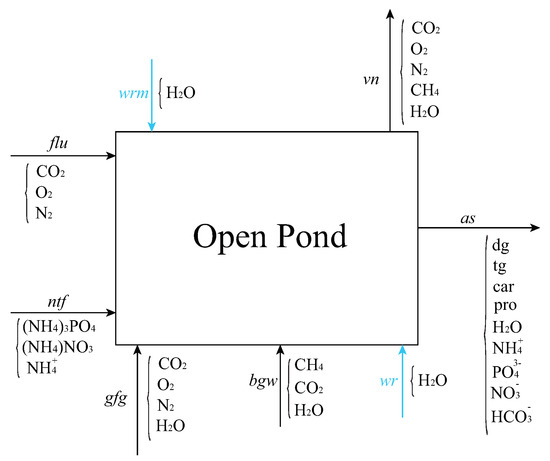
Figure 2.
Flow streams into and out of the open pond in the cultivation section of Figure 1. Inflows include a flue-gas stream from a carbon capture plan (flu), nutrients (ntf), flue gas from gas turbine (gfg), liquid stream from biogas upgrading (bgw), recycled water from dewatering section (wr), and makeup water (wrm). Outflows include a vent (vn) to account for water evaporation and unreacted gas emission into the atmosphere and algae slurry (as), non-aqueous phase of which contains diglycerides (dg), triglycerides (tg), proteins (pro), carbohydrates (car).
To estimate ion concentrations in the pond, we consider the following dissolution and dissociation equilibria
the equilibrium constants of which are summarized in Table 2. Given pH, the equilibrium concentration of all the ions can be obtained as functions of CO composition in the inflow and pressure of flue-gas streams.
We use expressions reported by Gebreslassie et al. [39] and Gong and You [8] to estimate the power and energy consumption of different units in the superstructure. The power consumption of pumps, floatation technology, and FPT are estimated
where
Here, is the index of the stream that the pump k operates on, P the power consumption in kW, the pump efficiency, the pump head in m, the floatation surface area in ft, the recycle percentage, the hydraulic loading in ton/day/ft, the required volume of the filter press in m, and the number of filtration cycles per day (see Table 3). The power (electric) consumption of all other units are estimated by
Table 3.
Parameters used to estimate the power and heat consumption of all the equipment in the superstructure shown in Figure 1.
The heat consumption of all the units in the superstructure is similarly calculated
where is the list of all the inflow streams of the equipment (or section) k, , and . The mass flowrates in these equations are measured in ton/day. Note that the power and heat consumption (see Table 3) of all the units in the remnant treatment, upgrading, and lipid-extraction sections are lumped together into a single variable; the subscripts RTS, UGS, and LES denote the respective processing section in Equations (26) and (27).
We evaluate the environmental impact of the downstream processing in Figure 1 by calculating the GWP according to
where
with , , and the contributions of the direct emission of greenhouse gases (GHG), the indirect emission of GHG due to power consumption, and the indirect emission of GHG due to heat consumption, all measured in hundred-year GWP of equivalent carbon dioxide (CO-eq). Here, is the list of all the GHGs in the superstructure that are released into the environment, the list of the streams through which GHGs are released, and is the mass fraction of species in the stream ; the damage factors associated with GHGs, electric consumption, and power consumption are denoted by , , and , respectively (see Table 4).
Table 4.
Parameters used to assess the global-warming potential of the superstructure shown in Figure 1 [8].
In this paper, we only focus on the environmental impacts of downstream processing. Therefore, we exclude the contribution of the CO in the flu-gas stream that is not sequestered in the cultivation section from GWP calculations. This implies that the unreacted CO in the cultivation section, which is released into the atmosphere, is not considered to be direct emission when calculating the GWP. Moreover, in our superstructure model, the stream vn (see Figure 2) is the only source of direct emission of GHGs. Thus, only reflects the amount of carbon fixation in the pond and the excess methane recycled from the biogas upgrading unit in the remnant treatment section.
2.2. Metabolic Model
We estimate the growth rate and metabolic fluxes in the open pond using a genome-scale model of C. reinhardtii, referred to as iRC1080 [33], which includes 1706 metabolites (175 of which constitute biomass) and 2191 reactions (76 exchange and demand reactions). Four major metabolite groups constitute the biomass in iRC1080: Carbohydrates, proteins, diacylglycerols, and triacylglycerols with weight fractions 56.09%, 14.10%, 7.12%, and 4.28%, respectively. The biomass in iRC1080 has no monoacylglycerols. In general, iRC1080 has higher coverage of genes, reactions, and lipid metabolic contents than previously published models. It explicitly accounts for all metabolites in lipid pathways, allowing for a more precise characterization of the alkyl esters produced in transesterification. Major lipid pathways that are incorporated into iRC1080 are those corresponding to ketoacyl lipids, fatty acyls, glycerolipids, glycerophospholipids, sphingolipids, sterol lipids, and prenol lipids. Autotrophic, heterotrophic, and mixotrophic growth modes are supported in iRC1080, enabling the prediction of light-intensity-dependent quantities. For example, the model can quantify important phenotypes, such as photosynthetic saturation and transitions from a carbon dioxide-producing to carbon dioxide-consuming metabolism (Experimental data used to validate the growth-rate predictions of iRC1080 were acquired from the strain UTEX2243 in the temperature range 23–27 C for a gas supply with 2.5% CO and photon fluxes in the range 42–170 (E/m/s) under 660 nm peak LED light). We only consider the autotrophic mode, assuming that the open pond operates during the photoperiod. The exchange fluxes associated with the consumption or production of X, HO, O, CO, HCO, NH, NO, and PO are determined by maximizing the growth rate in the autotrophic mode subject to stoichiometric constraints and inequalities representing uptake bounds that are estimated using Michaelis-Menten kinetic expressions. The maximum uptake rate of the last six species are
the maximum initial velocities and saturation constants of which are summarized in Table 5. We use Beer-Lambert law [40] to estimate how much photon flux algae can receive as a function of the biomass concentration and pond depth. Accordingly, the depth-averaged photon flux available to algae at a given time t (in hours) of the day is
where
is the scaled average light intensity in the pond with the length of photoperiod in hours, characteristic biomass concentration, Avogadro’s Number, ℏ Planck’s constant, light wave length, c speed of light, and surface light intensity. Here, is the biomass concentration scaled with (We use barred symbols to denote both time-averaged and scaled quantities. Throughout this paper, single-barred variables can either refer to time averaging or scaling. Adequate descriptions are provided to clarify whichever is relevant in the context. Double-barred variables are both time-averaged and scaled) and . The parameters and are taken from Yang [40].
Table 5.
Michaelis-Menten parameters for uptake rates of key species in Figure 2.
Fixing pH and the pressure of flue-gas streams, the maximum uptake rates for O, NH, NO, and PO remain constant, while for CO and HCO, they are parametrized with respect to the equilibrium concentration of CO in the pond. Treating CO equilibrium concentration and averaged photon flux as parameters, the metabolic network of C. reinhardtii can be formulated as a parametric linear program (LP)
where is the vector of reaction rates, , is the stoichiometry matrix, is the index set of reactions with a fixed lower bound, is the index set of reactions with a fixed upper bound, and is the index set of irreversible reactions with p and x the indices of average photon flux and biomass reaction, respectively. This model comprises metabolites and reactions in its non-standard form, where optimal metabolic pathways and reaction rates are determined by maximizing biomass production. Fixed upper and lower bounds in Equation (35) include fixed uptake-rate bounds and a lower bound on the ATP exchange reaction, accounting for ATP maintenance requirements [33].
Equation (35) can be simplified by establishing a range of pH, in which can be linearly expressed in terms of . Noting that , we find provided pH . We reformulate Equation (35) as a parametric LP with respect to using this approximation. Following the multi-parametric programming (MPP) algorithm of Akbari and Barton [44], a region of the parameter space of Equation (35), relevant to the operating conditions of the cultivation section, is partitioned into several critical regions (CRs), in which optimal reaction rates are expressed explicitly as affine functions of :
where is the parameter region of interest and are the respective CRs
with q the number of parameters. Here, , , , and are explicitly calculated offline using the algorithm of Akbari and Barton [44].
2.3. Resolving Transients
In this paper, we are only concerned with the steady-state optimization of algal biorefineries. However, the cultivation section can be hardly regarded as operating at a steady state due to significant hourly variations in growth rates resulting from light-intensity changes. A standard technique for handling these fluctuations in optimization problems is to discretize transient variables in time and assign a decision variable to each time interval representing the value of the corresponding variable at that time. This approach, however, is not tractable for most superstructure optimization problems of practical importance. This is because of the slow convergence rate of global optimization solvers caused by poor-quality convex under estimators arising from highly nonlinear equations (e.g., Equations (33) and (34)).
Alternatively, one can work with daily averaged heat- and mass-balance equations to avoid including hourly fluctuations in the optimization. This technique is especially helpful in techno-economic studies because their goal is to evaluate the economy of industrial plants on a yearly basis. For example, consider a sequential open raceway-pond configuration in Figure 3, where each pond is designed to achieve a daily periodic dynamic. The unsteady mass-balance equation around the kth pond reads
where is a conversion factor to ensure the consistency of concentration and metabolic-flux units, and i an index running over all the species involved in the mass balance. Here, and are the space-time and surface area of the kth pond with Q the volumetric flowrate of the inflow and outflow streams. Solving these unsteady equations provides much more information about instantaneous variations in the concentrations and reaction rates than needed for evaluating the yearly economic performance of biorefineries, and, therefore, unnecessarily complicates the analysis. However, at the superstructure level, one is generally concerned with daily averaged mass flowrates and seeks to relate averaged reaction rates to averaged concentrations , implicitly taking into account hourly fluctuations due to light-intensity changes and metabolic-mode alterations in the averaged quantities. In the present work, we adopt the latter approach and propose two computationally tractable optimization strategies to resolve the transients in open ponds.
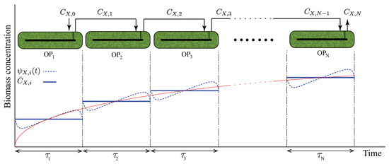
Figure 3.
Periodic time-varying concentration scheme used as the basis of Optimization Strategy II.
In Optimization Strategy I, we are only concerned with steady-state solutions; thus, we neglect changes in the photon flux due to variations of light intensity during a day. Accordingly, a time-averaged biomass concentration and light intensity is used in Equation (33) to estimate the average photon flux . Here, , A, and h are treated as decision variables, enabling the coupling of growth rates and the design parameters of the cultivation section. As a result, the growth state of algae, represented by CRs of the metabolic model in Section 2.2, is determined as part of the solution.
The foregoing strategy is suitable when yearly averaged estimates are of interest, and it does not address design parameters (e.g., the configuration of open ponds, number of ponds, biomass concentration) that depend on the hourly variations of growth rates. To demonstrate the capabilities of GEMs in predicting light-intensity-dependent metabolic rates, we study another computational strategy, which we refer to as Optimization Strategy II. Here, we consider a sequential open-pond configuration as shown in Figure 3, formulating TEA as a parametric MINLP, where the number of ponds, biomass concentration, pond depths, and pond surface areas are treated as parameters. This approach decouples CR identification (i.e., search for the metabolic state in which algae grows and corresponds to the optimal design and operating conditions of the cultivation section), which is necessary in Optimization Strategy I, from superstructure optimization, allowing for an offline calculation of growth rates. Given that the dynamics in the ponds are induced by sinusoidal light-intensity variations, we consider the following time-dependent concentrations and metabolic rates corresponding to the species i in the kth pond
where perturbations are assumed to be periodic with period , so that
Substituting Equations (39)–(42) in Equation (38) and integrating the resulting equations in time over , we obtain
Observe that the periodic perturbative approximations in Equations (39) and (40) have resulted in mass-balance equations that are in steady state with respect to the averaged quantities to second order in . Summing Equation (43) over k and neglecting the second- and higher-order terms in , we arrive at a modified version of Equation (8)
where we assumed that and with .
Since the parameter space for Optimization Strategy II (i.e., number of ponds, biomass concentration in each pond, pond surface areas, pond depths) is too large to exhaust, we make further simplifying assumptions, focusing on a particular scenario to illustrate the application of this strategy in TEA of biorefineries. We assume that the total surface area and the depth of each pond h are the same as their optimal values in Optimization Strategy I. We also assume that the averaged biomass concentrations are chosen such that all space times are equal to or as close to as possible. The first pond in the configuration shown in Figure 3 is an exception because the biomass concentration in its inflow stream is zeros. Therefore, achieving is not possible due to small growth-rate predictions from iRC1080, so we choose according to
where . For all other ponds, solves
Once the averaged concentrations and space times are identified, we seek to determine the number of sequential open ponds N that maximize the NPV.
2.4. Transesterification
Transesterification reactions play a central role in most biorefineries. They are reversible alkali-, acid-, or enzyme-catalyzed reactions of lipids with alcohols, producing biodiesel and glycerol. Monoglycerides, diglycerides, and triglycerides are major forms of lipids found in most algal species, requiring different stoichiometric amounts of alcohol to produce alkyl esters. For the upgrading section, we consider transesterification using methanol [3]
where , , and represent organic groups associated with mono, di, and triglycerides. Note that the two groups in Equation (48) and the three groups in Equation (49), which are lumped together for brevity, need not be identical. Biomass in iRC1080 comprises no monoglycerides, 81 diglyceride species, and 42 triglyceride species with organic groups of various lengths. Their respective alkyl esters constitute the biodiesel produced in the upgrading section of our superstructure model. To estimate the biodiesel mass flowrate from the transesterification reactor RX (see Figure 1), we use the stoichiometric coefficients in Equations (48) and (49) with the average molecular weights of and in all the foregoing glyceride species.
2.5. Optimization
This section provides the mathematical framework, in which to find optimal processing pathways that maximizes the NPV subject to technology choice, mass-, and energy-balance constraints. Binary variables corresponding to (i) technology choices and (ii) CRs of the parametric solutions of the metabolic network are two groups of discrete variables that arise in our superstructure model. Binary variables associated with technology choices are constrained such that each optimal pathway consists of only one technology in a given processing section. The operating conditions of the cultivation section determines the CR, the corresponding optimal reaction rates of which are to be used in Equation (8). As stated in Section 2.2, optimal reaction rates are parametrized with respect to the equilibrium concentration of CO in the pond and average photon flux . The former depends the composition of CO in the inflow streams, while the latter is determined by the pond depth h and biomass concentration (see Equations (33) and (34)). In Optimization Strategy I, We formulate the resulting optimization problem as a disjunctive programming problem [45,46], in which the inequities define disjunctions relating the operating conditions of the cultivation section to the reaction rates of the metabolic network.
Assumptions:
- Day-to-day variations of variables describing the dynamic state of open ponds are negligible compared to hourly variations during a day.
- The concentrations of all the species in the pond vary in a quasi-equilibrium manner.
- The length of photoperiod remains constant throughout the year.
- Nutrients (i.e., phosphate, nitrate, ammonia, and ammonium) and oxygen are available in excess of algae growth requirements, so that their concentrations remain fixed at the respective equilibrium values.
- Energy consumptions are linearly related to mass flowrates.
- Equipment purchase costs scale with mass flowrates.
Given parameters:
- Maximum tolerable CO emission to atmosphere from open pond.
- Solid contents of dilute algae-slurry stream, concentrated algae-slurry streams from dewatering technologies, and dried algae stream.
- Operating conditions of open pond, such as temperature and relative humidity.
- Length of photoperiod.
- Volume fraction of methane in biogas.
- Product distribution of anaerobic digester with respect to feed composition.
- Lipid and hexane recovery factors in lipid extraction and lipid-hexane separation columns.
- Fraction of hexane loss in lipid extraction column.
- Volumetric ratio of pressurized water to biogas feed.
- Air to fuel ratio of gas turbine combustion.
- Gas turbine efficiency.
- Mass flowrates of coagulant and polymer with respect to feed-mass flowrates.
- Reaction conversions in upgrading section.
- All economic parameters, such as interest rate, equipment reference purchase costs, cost indices, sizing factors, utility and material costs, and selling prices.
Decision variables:
- Methane recovery in biogas upgrading unit.
- Excess air in combustor.
- Split fractions of decanter and distillation columns in upgrading section.
- Heat and power consumptions.
- Mass flowrates of species.
- Capital and operating costs, revenue, and NPV.
- Technology selection.
- Critical region of metabolic network corresponding to optimal processing pathway.
- Biomass concentration, pond depth, and pond surface area.
- Reaction rates of species involved in mass balance of open pond.
This optimization problem can be formulated as a disjunctive MINLP, where disjunctions are associated with the CRs of the metabolic network.
where are continuous decision variables, binary variables associated with technology choices, binary variables associated with the CRs of the metabolic network, is the index set of technology alternatives in the processing section j, and are equality and inequality constraints consisting of mass-balance, energy-balance, and economic analysis equations, n the number of continuous decision variables, the total number of technology alternatives, the number of CRs, and the number of processing sections with technology alternatives. Note that in our simplified superstructure, there are technology alternatives only in the harvesting and dewatering section. Moreover, the parameters of the metabolic model are explicitly related to the CO and biomass concentrations in the pond and the pond depth, which are all continuous decision variables of the optimization problem. Incorporating a detailed metabolic model into the superstructure model, the composition of proteins, carbohydrates, lipids, and unreacted species in the dilute algae-slurry stream are determined as part of the optimization. The resulting disjunctive MINLP is formulated in the General Algebraic Modeling System (GAMS) 24.7 [47] and solved using the global solver BARON [48].
In Optimization Strategy II, growth rate and optimization calculations are decoupled. Therefore, the search for metabolic-mode alterations resulting from hourly light-intensity changes is performed offline when calculating averaged concentrations and averaged reaction rates. Consequently, the disjunctive statements in Equation (50) can be avoided. Accordingly, the optimization problem is simplified to
where represent the vector of parameters in Optimization Strategy II, as discussed in Section 2.3.
3. Results and Discussion
When CO is the only carbon source, photosynthesis involves a network of reactions, through which carbon dioxide and water are converted to glucose using the light energy. In general, the direction of the consumption and production reactions for carbon dioxide and oxygen is reversed when there is no sunlight. However, the transition from CO-producing to CO-consuming metabolic sates induced by light-intensity variations is sensitive to substrate and nutrient concentrations, the prediction of which is a nontrivial task. These phenotypes can be accurately quantified by GEMs, enabling reliable estimations of the cultivation productivity. Figure 4 shows the dependence of metabolic fluxes on the light intensity in C. reinhardtii when carbon dioxide is the only substrate. Observe that the transition between CO-consuming and CO-producing modes occurs at a positive photon flux, where the growth rate vanishes. Moreover, this model can predict the saturation photon flux (∼40 mE/gDW/hr) [33], beyond which no appreciable change in metabolic fluxes is observed with respect to the light intensity.
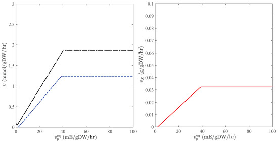
Figure 4.
Metabolic fluxes in the autotrophic mode when CO is the only carbon source. Left panel: consumption rate of CO (dashed) and production rate of O (dashed-dotted); Right panel: production rate of biomass. Equilibrium concentrations of O and CO are determined for a flue-gas stream that is fed into the pond at 0.5 atm and using Henry’s constants and atm/M [38] to estimate uptake bounds.
We first present parametric solutions of the autotrophic and heterotrophic modes for comparison, even though only autotrophic reaction rates are used in the superstructure. Polyhedral partitions of the parameter space for the autotrophic mode with respect to the CO-uptake bound and photon flux and the heterotrophic mode with respect to the CO- and O-uptake bounds, based on the maximization of biomass growth rate, are depicted in Figure 5. To ensure continuous parametric solutions for all decision variables, Equation (35) is solved with an auxiliary objective, the cost vector of which is constructed according to the algorithm of Akbari and Barton [44]. Solving this auxiliary LP is equivalent to imposing a priority order, with as many hierarchical levels as the number of decision variables, on the optimal solution set of Equation (35), such that the resulting lexicographic LP has a unique solution. During the photoperiod, algae absorb photons and CO to grow, produce energy, and secrete oxygen. Part of the energy is stored as starch within the cell. Accordingly, autotrophic metabolic modes depend on the photon flux and equilibrium concentration of CO in the extracellular environment, which, in turn, determines the CO-uptake bound (Figure 5, left panel). In contrast, during the night, algae consume oxygen and the stored starch to grow and produce CO, so heterotrophic metabolic modes are independent of the CO-uptake bound (Figure 5, right panel).
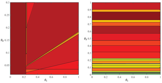
Figure 5.
Polyhedral partitions of the parameter space for a genome-scale model of C. reinhardtii (iRC1080) [33] based on autotrophic (left panel) and heterotrophic (right panel) maximum-growth objectives and an auxiliary objective with an equivalent cost vector that furnishes a continuous parametric solution with respect to all decision variables [44]. Here, , , and measure, respectively, the maximum uptake rate of carbon dioxide, photon flux, and maximum uptake rate of oxygen.
Explicit parametric solutions of iRC1080 are constructed offline and then used in a GAMS model of the biorefinery depicted in Figure 1. Table 6 summarizes key parameters used in our economic analysis. We treat recovery factors and split fractions as decision variables, not restricting them by equilibrium constraints for simplicity. Table 7 summarizes the results of Optimization Strategy I. Filtration is the optimal dewatering technology according to our model, agreeing with the results of Gebreslassie et al. [7] in the maximum NPV limit. Moreover, optimal recovery factors and split fractions ensure perfect separation as expected. In this context, the zero recovery factor of methane in the biogas upgrading unit is notable. This implies that recovering methane from residual biomass for power generation is uneconomical because of the high costs of the GT, agreeing with previous reports [1]. Furthermore, determining the optimal design of the open pond (e.g., surface area and depth) is nontrivial. One naturally expects that increasing the pond depth, surface area, and biomass concentration enhances the productivity; however, these also influence the reaction rates in a complicated way. For example, fixing the volume, shallow ponds have large surface area; thus, they need more makeup water to compensate for the water loss because of surface evaporation, significantly increasing the operating costs. On the other hand, surface evaporation can be reduced by using deep ponds with high algae concentrations; however, these also lower the amount of light energy that algae can absorb, decreasing the cultivation productivity.
Table 6.
Key economic parameters, material costs [7,8], and product selling prices. Ammonium phosphate (AP) and ammonium nitrate (AN) are the nutrients used for cultivation, while coagulant (COG), filtration polymer additive (FPA), and centrifugation polymer additive (CPA) are used for dewatering.
Table 7.
Summary of optimization results from Optimization Strategy I. Economic variables include annual project investment cost (APIC), annual operating cost (AOC), revenue (REV), annual actual profit after tax (APAT), and net present value (NPV).
The effect of the biodiesel selling price on economic variables are summarized in Table 8. All economic variables in our superstructure model exhibit a linear trend with respect to the biodiesel selling price. Fixing the glycerol price, the break-even price () of biodiesel from our superstructure model is ∼6500 , which is higher than the minimum prices reported in the literature for algal oils [5,6,50]. This is not surprising because these prices were obtained based on high-productivity estimates for open ponds. We also did not account for possible revenue that can be generated from selling protein and carbohydrate by-products. For example, Gallagher [50] reported a price range ∼1400–3000 $/ton assuming a productivity in the range ∼100–120 ton/ha/y. In contrast, the cultivation productivity in the present work (see Table 7) is directly calculated from the metabolic model, pond depth, and pond surface area. This low productivity is mainly due to the low lipid content (11.4% in weight fraction) of iRC1080. Clearly, producing biodiesel using available technologies is still too expensive to compete with conventional diesel (∼400 $/ton [50]). As has been recognized in the literature [1], algal biofuel can hardly be produced in practice at a competitive price to that of fossil fuel by relying only traditional products (e.g., biodiesel and glycerol); thus, the possibility of producing high-value products in the cultivation section has to be carefully examined.
Table 8.
The effect of biodiesel selling price on economic variables in Optimization Strategy I, including annual project investment cost (APIC), annual operating cost (AOC), revenue (REV), annual actual profit after tax (APAT), and net present value (NPV).
Figure 6 compares the energy consumption and operating costs of various processing sections in the superstructure. The cultivation and dewatering sections are by far the most energy consuming processes in our model, agreeing with the analysis of Gebreslassie et al. [7]. Accordingly, they are the most significant CO indirect emission sources of algal biorefineries and, thus, play an important role in the LCA of the superstructure. These sections also have the highest operating costs, which partly reflects their high energy consumption. In particular, the significantly large operating cost of the cultivation section reflects the cost of nutrients algae consume to grow.
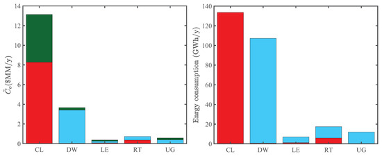
Figure 6.
Comparison of annual operating costs and energy consumption of the cultivation (CL), harvesting and dewatering (DW), lipid extraction (LE), upgrading (UG), and remnant treatment (RT) processing sections in Optimization Strategy I. Left panel: components of the reduced annual operating cost, including material (green), power (red), and heat (blue) costs. Right panel: power (red) and heat (blue) consumption.
To evaluate the environmental impacts of the maximum NPV design, we perform an LCA of the biorefinery. Figure 7a shows the contribution of each processing section to the total GWP. As expected, the cultivation and dewatering sections have the highest contributions because of their large heat and power consumption compared to other sections (see Figure 6). In addition to these indirect emission sources, the direct emission of unreacted carbon dioxide and methane (fed into the open pond through the recycle stream from the remnant treatment section) is a reason for the significantly large GWP of the cultivation section. Figure 7b shows the distribution of operating costs, revealing the bottlenecks for economic production of biodiesel. Power, heat, and nutrient costs contribute the most to the total operating costs, highlighting the importance of energy management and nutrient recovery strategies. Granted, thermal drying and LE from dried algae are too expensive to play any role in the future commercialization of algal biofuels. Efficient energy management in integrated biorefineries and lipid-extraction techniques that can process algae slurries with high liquid contents (e.g., HTL) are more promising for future designs [19,51,52].
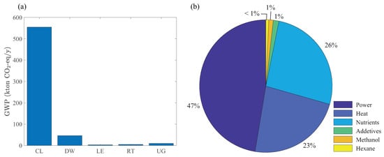
Figure 7.
(a) Global-warming potential of the processing sections in Figure 1, and (b) distribution of operating costs from Optimization Strategy I.
Before presenting the results of Optimization Strategy II, we examine the periodic unsteady-concentration hypothesis discussed in Section 2.3 by direct numerical computations. Figure 8 shows unsteady biomass concentrations in the first pond at various space times and initial concentrations. The initial concentrations set the scale for throughout the photoperiod. Here, we highlight two notable observations: First, for all initial concentrations, h furnishes that remain nearly constant during the photoperiod (except the beginning and end), which could have important design implications if the steady-state operation of open ponds are desired. Second, in the averaged concentration range 0.01–0.1 g/L and space-time range 20–24 h, there exists several solution pairs furnishing periodic unsteady-concentrations, which is the basis of Optimization Strategy II. Interestingly, Equation (45) provides the solution for the same operating conditions and design parameters as Figure 8, agreeing with the forging ranges obtained from direct numerical computations.
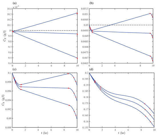
Figure 8.
Time-varying concentrations of algae growing in an open pond with no algae in the inflow stream (e.g., the first pond in Figure 3) and operating at mmol/L, h (upward), m, and h. Concentrations are plotted at (a) g/L, (b) g/L, (c) g/L, and (d) g/L. Red circles indicate transition points in the metabolic state of algae.
We formulated Optimization Strategy II in Section 2.3 to identify operating conditions and design parameters that can only be determined if hourly resolved growth rates are accounted for in the cultivation section. We introduced a particular scenario for maximizing NPV based on an interplay between the space times and averaged biomass concentrations in a sequential open-pond configuration. The space-time for each pond depends on the surface area, depth, and volumetric flowrates. However, for simplicity, we only considered space-time variations with respect to the flowrate at fixed surface area and depth, seeking biomass concentrations that minimize space times such that they are not smaller than the photoperiod. A key idea behind this approach is to restrict the search for maximum NPVs to scenarios that maximize the productivity of each pond (Note that is inversely proportional to the productivity of pond k at fixed h and . Of course, this proportionality should be regarded as a rough estimate and used as a guideline for designing scenarios because of the complicated relationship between the growth rate, pond depth, and biomass concentration) and maximally use the entire photoperiod length by design. The goal in Optimization Strategy II is then to find the number of open ponds in a sequential configuration (see Figure 3) that maximize NPV, where are chosen according to Equation (45). Figure 9a shows variations of NPV with respect to the number of open ponds. The respective averaged biomass concentrations for up to 35 consecutive reactors are plotted in Figure 9b. For the given operating conditions and design parameters, the maximum NPV $MM/y is achieved at with the corresponding total space-time h. Recall, the maximum NPV $MM/y from Optimization Strategy I was obtained based on a constant averaged biomass concentration with the total space-time h. This ∼27% increase in NPV reflects the potential economic benefits that can be gained from the variable biomass concentration scheme introduced in Section 2.3.
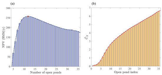
Figure 9.
Optimal number of open ponds in Optimization Strategy II for the sequential-pond configuration (see Figure 3) operating at mmol/L, m, and h. (a) NPV versus the number of sequential open ponds. Red circle indicates the number of ponds that furnish the maximum NPV. (b) Time-averaged concentration (scaled with g/L) distribution that ensures the most uniform space times across all the ponds. Polynomial fits (dashed lines) are plotted to show the trends.
4. Conclusions
Techno-economic and life-cycle analyses of algal biorefineries can benefit from accurate growth models for algae cultivation. Previous techno-economic studies were mostly based on unstructured growth models and empirical correlations that need fine-tuning for specific cultivation conditions and reactor designs. In contrast, genome-scale models can quantify the dependence of metabolic fluxes on the light intensity and substrate concentration, capturing metabolic-state transitions without relying on adjustable parameters. To leverage the predictive capabilities of genome-scale models for growth-rate estimation, we introduced a computational framework to integrate genome-scale and superstructure optimization models. This enabled the coupling of the design parameters of the cultivation and the stream flowrates of the superstructure. Our results suggest that the proposed implementation is computationally viable and applicable to larger superstructure models to provide more realistic economic assessments.
Overall, our results indicate that producing traditional products in biorefinaries using algal species with less than 35–40% lipid content is not economical. Several species of algae need to be systematically examined to identify the strains with desirable lipid content and determine other high-value products that can be potentially produced. In this context, genome-scale metabolic models are useful by providing a comprehensive description of all the metabolites a given species can produce with their respective stoichiometric coefficients in a reaction network. The optimization setting presented in this paper can then leverage the genomic information of reconstructed metabolic models to help accurately assess the economic impacts of producing novel products within the framework of carbon sequestration networks.
We studied a reduced superstructure model with traditional technology alternatives in the dewatering section to demonstrate how genome-scale models can be used to optimize the design and improve the performance of open raceway ponds. Emphasis was placed on the computational and optimization techniques, so we did not examine the latest and most efficient technologies for each processing section. Granted, the selling-price estimates in this paper can be improved if more advanced and efficient technologies are incorporated into the superstructure. In this context, two advanced cultivation and dewatering technologies that have recently emerged are notable [51]: (i) A novel sloped raceway pond with ∼200% higher productivity and ∼67% lower energy consumption than conventional raceway ponds, and (ii) a large-scale (∼10 gal/day) membrane-based harvesting and dewatering technology, reducing the energy consumption by more than an order of magnitude. Examining the economic and environmental impacts of these advanced technologies is a promising direction for future techno-economic studies of algal biorefineries.
Author Contributions
Mathematical-model and optimization problem formulation, A.A.; Mathematical and data analysis, A.A.; Computation, A.A.; Writing–original draft preparation, A.A.; Supervision, P.I.B.; Writing—review and editing, P.I.B.
Funding
This work was funded by the Cooperative Agreement between the Masdar Institute of Science and Technology (Masdar Institute), Abu Dhabi, UAE and the Massachusetts Institute of Technology (MIT), Cambridge, MA, USA - Reference 02/MI/MI/CP/11/07633/GEN/G/00 for work under the Second Five Year Agreement.
Conflicts of Interest
The authors declare no conflict of interest.
References
- Williams, P.J.l.B.; Laurens, L.M.L. Microalgae as biodiesel & biomass feedstocks: Review & analysis of the biochemistry, energetics & economics. Energy Environ. Sci. 2010, 3, 554–590. [Google Scholar] [CrossRef]
- Yue, D.; You, F.; Snyder, S.W. Biomass-to-bioenergy and biofuel supply chain optimization: Overview, key issues and challenges. Comput. Chem. Eng. 2014, 66, 36–56. [Google Scholar] [CrossRef]
- West, A.H.; Posarac, D.; Ellis, N. Assessment of four biodiesel production processes using HYSYS. Plant. Bioresour. Technol. 2008, 99, 6587–6601. [Google Scholar] [CrossRef]
- Pokoo-Aikins, G.; Nadim, A.; El-Halwagi, M.M.; Mahalec, V. Design and analysis of biodiesel production from algae grown through carbon sequestration. Clean Technol. Environ. Policy 2010, 12, 239–254. [Google Scholar] [CrossRef]
- Davis, R.; Aden, A.; Pienkos, P.T. Techno-economic analysis of autotrophic microalgae for fuel production. Appl. Energy 2011, 88, 3524–3531. [Google Scholar] [CrossRef]
- Amer, L.; Adhikari, B.; Pellegrino, J. Technoeconomic analysis of five microalgae-to-biofuels processes of varying complexity. Bioresour. Technol. 2011, 102, 9350–9359. [Google Scholar] [CrossRef]
- Gebreslassie, B.H.; Waymire, R.; You, F. Sustainable design and synthesis of algae-based biorefinery for simultaneous hydrocarbon biofuel production and carbon sequestration. AIChE J. 2013, 59, 1599–1621. [Google Scholar] [CrossRef]
- Gong, J.; You, F. Global optimization for sustainable design and synthesis of algae processing network for CO2 mitigation and biofuel production using life cycle optimization. AIChE J. 2014, 60, 3195–3210. [Google Scholar] [CrossRef]
- Martín, M.; Grossmann, I.E. Simultaneous optimization and heat integration for biodiesel production from cooking oil and algae. Ind. Eng. Chem. Res. 2012, 51, 7998–8014. [Google Scholar] [CrossRef]
- Severson, K.; Martín, M.; Grossmann, I.E. Optimal integration for biodiesel production using bioethanol. AIChE J. 2013, 59, 834–844. [Google Scholar] [CrossRef]
- Lardon, L.; Helias, A.; Sialve, B.; Steyer, J.P.; Bernard, O. Life-cycle assessment of biodiesel production from microalgae. Environ. Sci. Technol. 2009, 43, 6475–6481. [Google Scholar] [CrossRef]
- Mercer, P.; Armenta, R.E. Developments in oil extraction from microalgae. Eur. J. Lipid Sci. Technol. 2011, 113, 539–547. [Google Scholar] [CrossRef]
- Anastasakis, K.; Ross, A.B. Hydrothermal liquefaction of the brown macro-alga Laminaria saccharina: Effect of reaction conditions on product distribution and composition. Bioresour. Technol. 2011, 102, 4876–4883. [Google Scholar] [CrossRef] [PubMed]
- Vardon, D.R.; Sharma, B.K.; Scott, J.; Yu, G.; Wang, Z.; Schideman, L.; Zhang, Y.; Strathmann, T.J. Chemical properties of biocrude oil from the hydrothermal liquefaction of Spirulina algae, swine manure, and digested anaerobic sludge. Bioresour. Technol. 2011, 102, 8295–8303. [Google Scholar] [CrossRef] [PubMed]
- Frank, E.D.; Elgowainy, A.; Han, J.; Wang, Z. Life cycle comparison of hydrothermal liquefaction and lipid extraction pathways to renewable diesel from algae. Mitig. Adapt. Strateg. Glob. Chang. 2013, 18, 137–158. [Google Scholar] [CrossRef]
- Elliott, D.C.; Biller, P.; Ross, A.B.; Schmidt, A.J.; Jones, S.B. Hydrothermal liquefaction of biomass: Developments from batch to continuous process. Bioresour. Technol. 2015, 178, 147–156. [Google Scholar] [CrossRef]
- Biddy, M.J.; Davis, R.; Jones, S.B.; Zhu, Y. Whole Algae Hydrothermal Liquefaction Technology Pathway; Pacific Northwest National Lab. (PNNL): Richland, WA, USA, 2013. [Google Scholar] [CrossRef]
- Barlow, J.; Sims, R.C.; Quinn, J.C. Techno-economic and life-cycle assessment of an attached growth algal biorefinery. Bioresour. Technol. 2016, 220, 360–368. [Google Scholar] [CrossRef]
- Elliott, D.C. Review of recent reports on process technology for thermochemical conversion of whole algae to liquid fuels. Algal Res. 2016, 13, 255–263. [Google Scholar] [CrossRef]
- Orfield, N.D.; Fang, A.J.; Valdez, P.J.; Nelson, M.C.; Savage, P.E.; Lin, X.N.; Keoleian, G.A. Life cycle design of an algal biorefinery featuring hydrothermal liquefaction: Effect of reaction conditions and an alternative pathway including microbial regrowth. ACS Sustain. Chem. Eng. 2014, 2, 867–874. [Google Scholar] [CrossRef]
- Ou, L.; Thilakaratne, R.; Brown, R.C.; Wright, M.M. Techno-economic analysis of transportation fuels from defatted microalgae via hydrothermal liquefaction and hydroprocessing. Biomass Bioenergy 2015, 72, 45–54. [Google Scholar] [CrossRef]
- Kothari, R.; Pandey, A.; Ahmad, S.; Kumar, A.; Pathak, V.V.; Tyagi, V.V. Microalgal cultivation for value-added products: A critical enviro-economical assessment. 3 Biotech 2017, 7, 243. [Google Scholar] [CrossRef]
- Dong, T.; Knoshaug, E.P.; Davis, R.; Laurens, L.M.L.; Van Wychen, S.; Pienkos, P.T.; Nagle, N. Combined algal processing: A novel integrated biorefinery process to produce algal biofuels and bioproducts. Algal Res. 2016, 19, 316–323. [Google Scholar] [CrossRef]
- Juneja, A.; Murthy, G.S. Evaluating the potential of renewable diesel production from algae cultured on wastewater: Techno-economic analysis and life cycle assessment. AIMS Energy 2017, 5, 239–257. [Google Scholar] [CrossRef]
- Hernaandez-Calderoon, O.M.; Ponce-Ortega, J.M.; Ortiz-del Castillo, J.R.; Cervantes-Gaxiola, M.E.; Milaan-Carrillo, J.; Serna-Gonzalez, M.; Rubio-Castro, E. Optimal design of distributed algae-based biorefineries using CO2 emissions from multiple industrial plants. Ind. Eng. Chem. Res. 2016, 55, 2345–2358. [Google Scholar] [CrossRef]
- Gonzalez-Bravo, R.; Sauceda-Valenzuela, M.; Mahlknecht, J.; Rubio-Castro, E.; Ponce-Ortega, J.M. Optimization of Water Grid at Macroscopic Level Analyzing Water–Energy–Food Nexus. ACS Sustain. Chem. Eng. 2018, 6, 12140–12152. [Google Scholar] [CrossRef]
- Wang, B.; Gebreslassie, B.H.; You, F. Sustainable design and synthesis of hydrocarbon biorefinery via gasification pathway: Integrated life cycle assessment and technoeconomic analysis with multiobjective superstructure optimization. Comput. Chem. Eng. 2013, 52, 55–76. [Google Scholar] [CrossRef]
- O’Connell, D.; Savelski, M.; Slater, C.S. Life cycle assessment of dewatering routes for algae derived biodiesel processes. Clean Technol. Environ. Policy 2013, 15, 567–577. [Google Scholar] [CrossRef]
- Liu, P.; Gerogiorgis, D.I.; Pistikopoulos, E.N. Modeling and optimization of polygeneration energy systems. Catal. Today 2007, 127, 347–359. [Google Scholar] [CrossRef]
- Chen, Y.; Adams, T.A.; Barton, P.I. Optimal design and operation of flexible energy polygeneration systems. Ind. Eng. Chem. Res. 2011, 50, 4553–4566. [Google Scholar] [CrossRef]
- Baliban, R.C.; Elia, J.A.; Misener, R.; Floudas, C.A. Global optimization of a MINLP process synthesis model for thermochemical based conversion of hybrid coal, biomass, and natural gas to liquid fuels. Comput. Chem. Eng. 2012, 42, 64–86. [Google Scholar] [CrossRef]
- Esener, A.A.; Roels, J.A.; Kossen, N.W.F. Theory and applications of unstructured growth models: Kinetic and energetic aspects. Biotechnol. Bioeng. 1983, 25, 2803–2841. [Google Scholar] [CrossRef]
- Chang, R.L.; Ghamsari, L.; Manichaikul, A.; Hom, E.F.Y.; Balaji, S.; Fu, W.; Shen, Y.; Hao, T.; Palsson, B.; Salehi-Ashtiani, K.; et al. Metabolic network reconstruction of Chlamydomonas offers insight into light-driven algal metabolism. Mol. Syst. Biol. 2011, 7, 518. [Google Scholar] [CrossRef]
- Akbari, A.; Barton, P.I. Incorporating detailed metabolic models into superstructure optimization of biorefineries. In Computer Aided Chemical Engineering; Elsevier: Amsterdam, The Netherlands, 2017; Volume 40, pp. 2143–2148. [Google Scholar] [CrossRef]
- Gomez, J.A.; Höffner, K.; Barton, P.I. From sugars to biodiesel using microalgae and yeast. Green Chem. 2016, 18, 461–475. [Google Scholar] [CrossRef]
- Sinnott, R.K.; Towler, G. Chemical Engineering Design: SI Edition; Elsevier: Amsterdam, The Netherlands, 2009. [Google Scholar]
- Lurie, M.; Michailoff, N. Evaporation from free water surface. Ind. Eng. Chem. 1936, 28, 345–349. [Google Scholar] [CrossRef]
- Perry, R.H. Perry’s Chemical Engineers’ Handbook; McGraw-Hill: New York, NY, USA, 1984. [Google Scholar]
- Gebreslassie, B.H.; Slivinsky, M.; Wang, B.; You, F. Life cycle optimization for sustainable design and operations of hydrocarbon biorefinery via fast pyrolysis, hydrotreating and hydrocracking. Comput. Chem. Eng. 2013, 50, 71–91. [Google Scholar] [CrossRef]
- Yang, A. Modeling and evaluation of CO2 supply and utilization in algal ponds. Ind. Eng. Chem. Res. 2011, 50, 11181–11192. [Google Scholar] [CrossRef]
- Hein, M.; Pedersen, M.F.; Sand-Jensen, K. Size-dependent nitrogen uptake in micro-and macroalgae. Mar. Ecol. Prog. Ser. 1995, 118, 247–253. [Google Scholar] [CrossRef]
- Galván, A.; Quesada, A.; Fernández, E. Nitrate and nitrite are transported by different specific transport systems and by a bispecific transporter in Chlamydomonas reinhardtii. J. Biol. Chem. 1996, 271, 2088–2092. [Google Scholar] [CrossRef]
- Nyholm, N. Kinetics of phosphate limited algal growth. Biotechnol. Bioeng. 1977, 19, 467–492. [Google Scholar] [CrossRef]
- Akbari, A.; Barton, P.I. An improved multi-parametric programming algorithm for flux balance analysis of metabolic networks. J. Optim. Theory Appl. 2018, 1–36. [Google Scholar] [CrossRef]
- Lee, S.; Grossmann, I.E. New algorithms for nonlinear generalized disjunctive programming. Comput. Chem. Eng. 2000, 24, 2125–2141. [Google Scholar] [CrossRef]
- Trespalacios, F.; Grossmann, I.E. Review of mixed-integer nonlinear and generalized disjunctive programming methods. Chem. Ing. Tech. 2014, 86, 991–1012. [Google Scholar] [CrossRef]
- Bussieck, M.R.; Meeraus, A. General algebraic modeling system (GAMS). In Modeling Languages in Mathematical Optimization; Springer: Berlin/Heidelberg, Germany, 2004; pp. 137–157. [Google Scholar] [CrossRef]
- Tawarmalani, M.; Sahinidis, N.V. A polyhedral branch-and-cut approach to global optimization. Math. Program. 2005, 103, 225–249. [Google Scholar] [CrossRef]
- Pinedo, J.; Prieto, C.G.; D’Alessandro, A.A.; Ibáñez, R.; Tonelli, S.; Díaz, M.S.; Irabien, Á. Microalgae biorefinery alternatives and hazard evaluation. Chem. Eng. Res. Des. 2016, 107, 117–125. [Google Scholar] [CrossRef]
- Gallagher, B.J. The economics of producing biodiesel from algae. Renew. Energy 2011, 36, 158–162. [Google Scholar] [CrossRef]
- Hazlebeck, D.; Corpuz, R.; Pinowska, A.; Rickman, B.; Traller, J. Development of Algal Biomass Yield Improvements in an Integrated Process; Global Algae Innovations: San Diego, CA, USA, 2018. [Google Scholar] [CrossRef]
- Chandra, R.; Iqbal, H.M.N.; Vishal, G.; Lee, H.S.; Nagra, S. Algal biorefinery: A sustainable approach to valorize algal-based biomass towards multiple product recovery. Bioresour. Technol. 2019. [Google Scholar] [CrossRef]


© 2019 by the authors. Licensee MDPI, Basel, Switzerland. This article is an open access article distributed under the terms and conditions of the Creative Commons Attribution (CC BY) license (http://creativecommons.org/licenses/by/4.0/).