Abstract
Phosphorus is an essential resource for numerous industrial applications. However, its uneven global distribution makes Europe heavily dependent on imports. Recovering phosphorus from waste streams is therefore crucial for improving resource security. The FlashPhos project addresses this challenge by developing a process to recover phosphorus from sewage sludge, in which phosphorus-rich slag is produced in a flash reactor and subsequently reduced in a Submerged Arc Furnace (SAF). In this process, approximately 250 kg/h of sewage sludge is converted into slag, which is further processed in the SAF to recover about 8 kg/h of white phosphorus. This work focuses on the development of a computational model of the SAF, with particular emphasis on slag behaviour. Due to the extreme operating conditions, which severely limit experimental access, a numerically efficient three-dimensional CFD model was developed to investigate the internal flow of the three-phase, AC-powered SAF. The model accounts for multiphase interactions, dynamic bubble generation and energy sinks associated with the reduction reaction, and Joule heating. A temperature control loop adjusts electrode currents to reach and maintain a prescribed target temperature. To further reduce computational cost, a novel simulation approach is introduced, achieving a reduction in simulation time of up to 300%. This approach replaces the solution of the electric potential equation with time-averaged Joule-heating values obtained from a preceding simulation. The system requires transient simulation and reaches a pseudo-steady state after approximately 337 s. The results demonstrate effective slag mixing, with gas bubbles significantly enhancing flow velocities compared to natural convection alone, leading to maximum slag velocities of 0.9–1.0 m/s. The temperature field is largely uniform and closely matches the target temperature within ±2 K, indicating efficient mixing and control. A parameter study reveals a strong sensitivity of the flow behaviour to the slag viscosity, while electrode spacing shows no clear influence. Overall, the model provides a robust basis for further development and future coupling with the gas phase.
1. Introduction
1.1. Background and Motivation
The primary use cases for Submerged Arc Furnaces (SAFs) are in the ferroalloy production and phosphorus production. Phosphorus is a valuable resource that is utilized in the fertilizer industry, as well as in the manufacturing of flame retardants and food additives [1,2,3]. Due to the limited availability of natural phosphorus in the form of calcium phosphate, which is used to produce white phosphorus (), there is a growing interest in finding alternative sources of phosphorus, including recovery. Especially in Europe, there is a big push towards finding such an alternative due to the high reliance on phosphorus imports.
A promising approach that has emerged in recent years is the use of sewage sludge as a phosphorus source [4,5,6]. In one conceptual process (Figure 1), the dried and ground sewage sludge is first incinerated in a flash reactor, producing phosphorus-containing slag and fuel gas [7,8]. The raw fuel gas from the flash reactor is further processed and utilised as a source of heat and clean fuel gas at the host plant, while the recovered heavy metals can be repurposed for industrial applications.
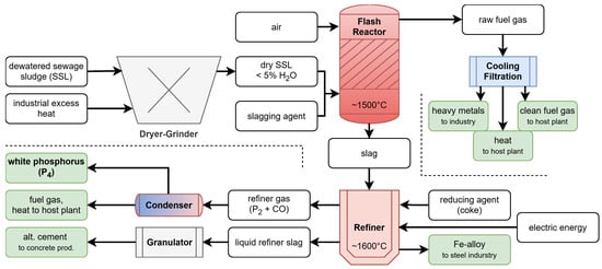
Figure 1.
Overview of the FlashPhos process for the recovery of white phosphorus from sewage sludge. White: educts, green: products.
The slag is subsequently refined in a SAF, following a process that can be represented by the following model reaction:
where carbon () is supplied by the electrodes and added coke, which reacts with the phosphorus-containing slag (here assumed to be —calcium phosphate) from the flash reactor to produce diphosphorus () and carbon monoxide () in gaseous form and as liquid product. The reaction equation in the presented work Equation (1) was also used by Askarizadeh et al. [9] to predict the phosphorus recovery from sewage sludge and is similar to the reaction used for phosphorus production from fluorapatite [10]. Due to the high temperatures, it is expected that predominantly is formed instead of white phosphorus () as is favoured and stable at high temperatures but readily recombines to upon cooling [11]. Additionally, ferrophosphorus is produced as a by-product, which can be utilized in the steel industry.
The refiner gas is subsequently condensed, allowing diphosphorus () to recombine into white phosphorus () while also providing fuel gas to the host plant. The liquid refiner slag is cooled, granulated and repurposed as an alternative cement binder in concrete production. The recovery percentage of the phosphorus present in the sewage sludge is approximately 75%, depending on the composition. This can be estimated from the study by Kotze et al. [12].
1.2. Submerged Arc Furnace Structure and Multiphase Flow
The SAF is a variant of the conventional Electric Arc Furnace (EAF), in which the electrodes are submerged in a packed bed or molten slag, depending on the application. This configuration leads to different heating mechanisms compared to the standard EAF. The primary heat source for the EAF is the forming of electric arcs, whereas the main heat source for the SAF presented in this study is Joule-heating (resistive heating) [13]. The SAF used for phosphorus recovery in this study is a circular three-phase furnace, where a multiphase system consisting of ferrophosphorus, slag and gas (mainly and ) is present. The geometry and electrode placement influence the heating distribution, bubble formation, and resulting flow patterns. In addition, the reduction reaction introduces a local energy sink and generates gas bubbles within the slag, which further affects the flow behaviour.
Fluid flow in the SAF is driven by multiple interacting mechanisms [14,15]:
- Bubble-induced stirring, resulting from the bubble generation caused by the reduction reaction. Rising gas bubbles impart a substantial amount of their momentum to the surrounding slag, therefore increasing the velocities in bubble-rich regions and enhancing mixing.
- Natural buoyancy, which is caused by density differences induced by temperature gradients.
- Electromagnetic stirring, arising from the electric current, though typically small compared to bubble- and buoyancy-driven effects.
Depending on the furnace geometry and the modelled process, the contribution of these mechanisms differs. In the presented model, the flow is mainly driven by the bubbles with secondary contributions by natural buoyancy, while electromagnetic stirring does not occur. These mechanisms interact in a complex multiphase environment with moving interfaces, making accurate modelling challenging.
Modelling challenges include capturing multiphase interfaces, coupling the energy sink from the chemical reaction to bubble generation, accurate bubble modelling and their interaction with the continuous phase, and maintaining numerical stability and efficiency. However, accurately capturing these interactions is essential to predict the temperature and velocity distribution, both of which affect the efficiency of phosphorus recovery. Given that this plant is a first of its kind and only limited data is available in the literature, a three-dimensional Computational Fluid Dynamics (CFD) model was developed. CFD models are widely used in both research and industry, as they enable the investigation of complex phenomena, parameter variations, and system behaviour that are difficult to measure directly due to extreme operating conditions [16,17,18]. The goal is to capture multiple key phenomena—including electric potential, multiphase flow, energy sink and bubble generation due to the chemical reaction and the influence of the furnace control—while maintaining computational efficiency and a reasonable simulation time. However, due to limited experimental data for this novel process, boundary condition specification and model validation is further complicated.
1.3. Computational Modelling of Submerged Arc Furnaces
Over the years, various research studies have been conducted, modelling and investigating the behaviour of SAFs for various applications. In contrast to the conventional EAF used for steel production—where the heat is predominantly generated by the electric arcs—in a Submerged Arc Furnace, the heat is mainly generated by Joule-heating within the slag layer [14]. The flow dynamics within the slag layer are mainly driven by buoyancy forces and bubble-induced stirring, resulting from the released gas [19,20]. In some cases, secondary stirring forces driven by electromagnetic Lorentz-type forces may arise and need consideration. However, the existing literature finds these electromagnetic forces in most cases to be negligible compared to buoyancy effects and bubble-stirring [14,19,20,21,22]. In this study, bubble-induced stirring is explicitly incorporated into the model, as it is expected to play a more significant role due to the specific geometry and process conditions of the system under investigation.
Sheng et al. [14,20] performed an experimental and mathematical investigation of a six-in-line (six electrodes placed in one line) electric furnace for the smelting of nickel matte. Their study revealed a substantial electric potential drop at the electrode surface, which was attributed to arcing through the carbon monoxide that forms as a result of the electrode’s oxidation. Furthermore, it was determined that the motion of the slag is mainly driven by the gas bubbles that are formed at the electrode surface. Natural convection plays a less significant role in this process. The alternating current in their study was replaced by an equivalent direct current as only steady state solutions were of interest.
The studies carried out by Bezuidenhout et al. [19,23] investigated an electric furnace used for platinum smelting. They applied a 3D transient CFD simulation, comparing different electrode immersion depths, modelled the energy sink due to smelting and tapping, and assessed the impact of including or excluding carbon monoxide () bubbles. They also found that the bubbles have a significant effect on both the maximum temperature and bath mixing, highlighting that bubble dynamics should not be neglected in accurate furnace modelling. A novelty in their work was the modelling of the interface between the layers as a dynamic interface, unlike previous studies, which incorporated a no-slip wall.
Karalis et al. [15] performed a 2D steady state CFD analysis of an industrial electric arc furnace. Their study applied a constant electric potential on the electrodes to investigate the effects of different electrode shapes and immersion depths, as well as the impact of slag properties on Joule-heating. bubbles were not included in their model.
Various studies investigating bubble columns, steel ladles, and two-phase stirred tanks emphasised the importance of bubble–fluid interaction on the flow field, therefore encouraging the inclusion of bubble effects in the analysis [24,25,26].
While these studies provide valuable insights, several key factors that significantly influence the process modelled in this work have only been considered briefly or overlooked entirely. These include, but are not limited to:
- The absence of process data, as the investigated concept represents a novel approach.
- The simplified treatment of bubble generation in current models, despite its expected importance for the present process, since the reduction reaction is not limited to the electrode surface.
- The modelling of the energy sink primarily as a volumetric distribution, without considering the local cell temperature.
- The lack of furnace control simulations aimed at reaching and maintaining a specified process temperature in the existing literature.
1.4. Objective of This Study
The objective of this study is to develop a three-dimensional CFD model of a SAF for phosphorus recovery that explicitly addresses the limitations identified in previous work while maintaining computational efficiency. The model introduces a more detailed, dynamic representation of the energy sink associated with the reduction reaction and a direct coupling to the bubble generation. In addition, a furnace control strategy is implemented to reach and maintain a predefined operation point under transient conditions. The model is applied to investigate the influence of key process parameters, namely electrode spacing and slag viscosity, on flow behaviour and temperature distribution. Additionally, a novel approach to further reduce simulation time by using Mean-Joule-heating (MJH) as a source term is proposed. The primary focus of this study was the accurate modelling of the slag, as its velocity and temperature distribution have a significant impact on the phosphorus recovery efficiency. Therefore, to reduce model complexity and the computational cost, shortcomings in the representation of the gas phase were accepted. However, the model is capable of including accurate modelling of the gas phase if the transport of the gas to further processing is of interest. These additions are by no means standard in the used commercial CFD software, ANSYS Fluent 2024 R1, and therefore require manual implementation via so-called User-Defined Functions (UDFs). First, the numerical model and its implementation are described. Then, the results of the furnace and the performance of the furnace control strategy is analysed. Finally, a parameter study is conducted to assess the sensitivity of the process to selected parameters.
2. Model Development and Methods
2.1. Geometry and Materials
The presence of a circular three-phase electric current necessitates the use of a 3D model of the refiner, as the current flow path varies in 3D space, depending on the current phase [19,23]. The refiner is composed of multiple layered walls, incorporating a complex design. Given the predominant interest in the fluid flow of the slag, where the reduction reaction takes place and the phosphorus is produced, it was decided to only model the innermost furnace lining. This includes the furnace shell as well as the lid. The model, which is around 1 m in diameter on the inside and a bit over 1 m in height, as well as the different materials, are shown in Figure 2. Note that the height of the phases shown represents their initialized levels. The two cutting planes are used to evaluate the results, while the radius R denotes the circle on which the electrodes are arranged. The effect of varying electrode distances is investigated in the subsequent parameter study (see Section 3.6). The electrodes are composed of graphite and the furnace lining is also carbon-based.
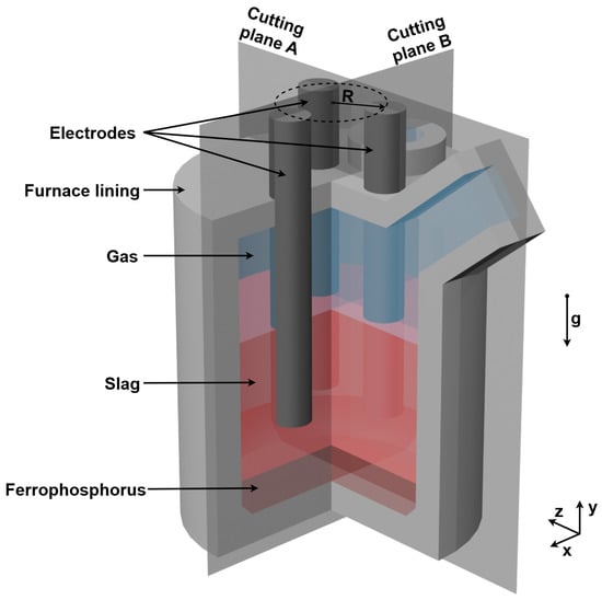
Figure 2.
Furnace geometry and materials.
The inputs and outputs of the refiner are shown in Figure 1. The phases present in the SAF are as follows:
- The gas phase, which is composed of a mixture of carbon monoxide () and diphosphorus (), as is the gaseous and stable form of at high temperatures [11]. Due to the high temperatures, the gas mixture was modelled as an ideal gas, which was also carried out by Scheepers et al. [10].
- The slag, which is supplied from the flash reactor and consisting of the residues of dried and burnt sewage sludge.
- The ferrophosphorus, which is formed as an unwanted by-product when iron (Fe) is present in the slag since it binds phosphorus and therefore reduces the recoverable amount of phosphorus.
The properties of the different materials were obtained from the literature and manufacturers’ data sheets, where such information was available. In order to capture buoyancy, one of the main drivers of the flow, it is necessary to allow the density of the slag to vary with temperature. A summary of the physical properties used is shown in Table 1. The manufacturer provided the values for the furnace lining. However, the data sheet is not publicly available.

Table 1.
Physical properties of the materials used.
2.2. Computational Grid
The simulation domain, also called mesh, was created using the implemented meshing tool of ANSYS Fluent 2024 R1 and consisted of 477,901, mostly polyhedral cells with sufficient orthogonal quality (see Figure 3). To better capture high gradients of the electric current in the vicinity of the electrodes, the mesh was refined in this region.
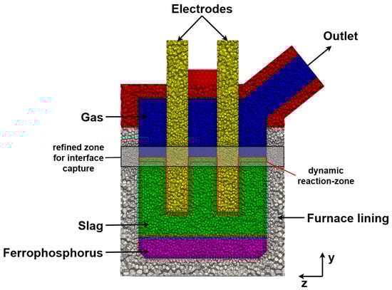
Figure 3.
Computational domain showing the spatial discretization of the system including the refined zone for interface capture (black) and the dynamic reaction-zone (red) for calculating the energy sink (Section 2.8.2).
Special attention was also given to the slag–gas interface, where significant movement is anticipated due to bubble formation. To accurately account and resolve this movement, a broad layer around the interface was refined. The dynamic reaction zone is also highlighted in Figure 3, which is important, as this is where the energy sink (Section 2.8.2) and bubble generation (Section 2.8.3) are dynamically calculated and incorporated into the model via UDFs.
2.3. Boundary Conditions
The applied boundary conditions (BCs) are shown in Figure 4. Surfaces of the same colour indicate the same BC. At the top of the lid, including the geometry around the inlet and outlet (W1), convection was considered with a free stream temperature of 80 °C and a heat transfer coefficient of 2 W/(m2 K). This value for the heat transfer coefficient is adopted from Karalis et al. [15] and although not mentioned, it is expected that it already considers the additional layers of insulation, as it is lower than typical.
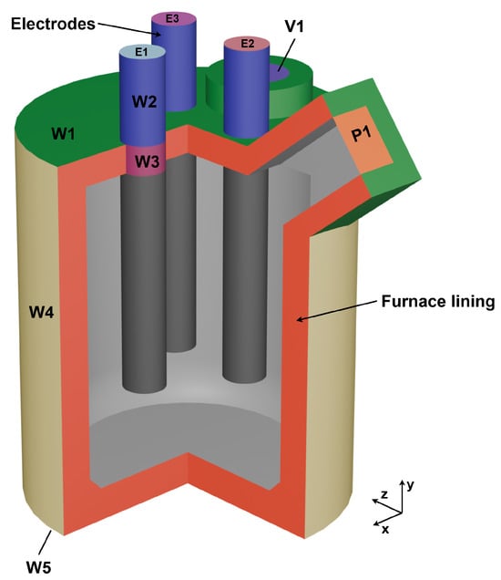
Figure 4.
Model overview showing the applied BCs for every component.
The outer furnace wall (W4) has been assigned a constant heat flux of −3049 W/m2. This heat flux was calculated and derived from a prior simulation of the heat transfer through the different furnace walls and was recalculated to correspond to the inner furnace lining represented in the current model. The outer furnace ground (W5) was considered to be adiabatic as in real life operation multiple insulation layers are present and the heat flux lost over the ground can be considered negligible.
The top of the electrodes (E1-3) are set according to the current Equation (14), only differing in phase lag, which is discussed in greater detail in Section 2.8. The walls of the electrodes above the furnace top (W2) are cooled and set to a constant heat flux of −47,900 W/m2, which was also determined in a prior simulation. Additionally the current density was set to 0 A/m2 (electrically isolated) to prevent any unintended current leakage. The same applies for the face, where the electrode passes through the lid (W3), as not defining a current density of 0 A/m2 would lead to a short circuit, as the complete outer furnace shell (W1, W4, W5) was set to an electric potential of 0 V, thus being grounded. The velocity inlet (V1) was set to 0.001 m/s and the pressure outlet (P1) to 0 Pa (relative pressure).
In actual operation, V1 is primarily used to introduce coke into the system, which is essential for the process (Figure 1), rather than serving as a true gas inlet. However, a small inlet velocity was applied in the simulation to enhance numerical stability and convergence in the gas phase. This inlet velocity defines the initial flow direction of the gas phase before the flow field is fully developed and thus stabilizes the numerical solution during the early stages of the simulation. All other walls not mentioned (grey) were set to coupled regarding the thermal and potential boundary conditions.
2.4. Flow Modelling
In CFD, a system of conservation equations has to be solved in a discretized form. As the power input is due to a time-dependent three-phase electric current, these equations have to be solved in a transient manner until a pseudo-steady state is reached. The system of conservation equations for a transported variable is generalized by Equation (2) [32]:
where stands for the transported quantities U, V, and W, which represent the velocity component of the three coordinate dimensions and yields the momentum equation. For , the continuity equation is obtained. From a physical standpoint, the first term on the left-hand side represents transient variations, while the second term accounts for convection. On the right-hand side, the first term addresses diffusion, and S allows for the implementation of additional source terms [32].
This generalized form can be split into the conservation of mass and momentum. Additionally, due to the presence of Joule-heating and additional energy sinks, the energy equation, Equation (3), plays a crucial role and should be explicitly mentioned.
The form of the energy equation solved in Fluent [33] is as follows:
where is the sensible heat of the species j, and is the diffusion flux of species j. Physically, the first term on the left-hand side accounts for the local change in energy, while the second term corresponds to the convective change. On the right-hand side, the terms from left to right represent the energy transfer due to conduction, species diffusion, viscous dissipation, and additional sources or sinks.
Consideration of Turbulence
In consideration of the furnace dimensions, the anticipated flow velocities within the slag, and its relatively high viscosity, an assessment based on Rayleigh and Reynolds numbers indicates that buoyancy-driven convection in the slag bath is predominantly laminar. While gas evolution introduces additional momentum and may locally disturb the flow, both dimensionless numbers suggest that fully developed turbulence is unlikely, and at most weakly transitional behaviour may occur in localized regions.
To evaluate the influence of such effects, the standard k– model and the transitional k–– turbulence model was tested. The k– model produced unrealistic temperature distributions due to the overly excessive diffusive behaviour. The resulting flow fields using the transitional model were found to be very similar to those obtained with the laminar model. However, the transitional model introduced non-physical artefacts arising from the multiphase setup, including artificially elevated eddy viscosity within the stagnant ferrophosphorus phase and unrealistic flow near the slag-ferrophosphorus interface. Consequently, the laminar flow assumption was retained, as it provides a physically consistent description without introducing numerical distortions. Similar conclusions regarding laminar slag flow have been reported by Bezuidenhout et al. [19,23].
The gas phase above the slag is included primarily to enable deformation and tracking of the slag–gas interface within the VOF framework and to allow for future model extensions. However, the primary interest of this study is the flow behaviour of the slag. Therefore, due to the large density difference between the gas and slag phases, momentum transfer from the gas to the slag is negligible. As a result, the slag flow is governed by buoyancy forces and bubble-induced mixing, while shear stresses originating from the gas phase play an insignificant role. Under these conditions, turbulence generated in the gas phase does not meaningfully influence the slag flow field or the interface dynamics relevant to this study.
Introducing turbulence modelling in the gas phase would therefore not improve the physical fidelity of the slag flow predictions and may instead introduce additional numerical problems due to the multiphase approach and increase computational cost without affecting the quantities of interest. Accordingly, the gas phase was also treated as laminar. This modelling choice is consistent with the physical dominance of the slag phase and does not affect the conclusions of the present study. This assessment is further supported by the test case employing a transitional turbulence model for all phases, which did not show meaningful differences in the slag flow field.
2.5. Multiphase Modelling
2.5.1. Liquid Phases
The presence of multiple phases requires the use of a multiphase modelling approach. The Volume of Fluid (VOF) model was chosen as it has proven to be a reliable and computationally cost-effective solution for modelling immiscible liquids [34]. VOF is a surface-tracking technique, which applies a Euler–Euler approach. Its use case is for two or more immiscible fluids where the interface between the fluids is of interest [33].
The bottom layer in the considered system is represented by ferrophosphorus, above which is the layer of interest—slag—and the top is represented by a layer of gas. The interface tension between the multiphase layers was estimated and set to 400 mN/m, relating to the work of Safarian et al. [35], Sunderström et al. [36], and Jønck [27]. These studies were chosen as references, as they investigate systems with similarly high temperatures and comparable slag and gas phase compositions.
2.5.2. Gas Bubbles
The generation of bubbles as a consequence of the reduction reaction exerts a substantial influence on the flow dynamics within the slag, therefore requiring their consideration. The implementation of the bubbles and their generation are discussed in greater detail in Section 2.8.3. For implementation into the CFD model, the Discrete Phase Model (DPM) was used. The DPM model tracks a discrete phase (in this case, the bubbles) inside a continuous phase (slag).
2.6. Radiation
In many industrial processes the temperatures involved are sufficiently high that thermal radiation becomes a significant mode of heat transfer. In contrast to conduction or convection, thermal radiation does not rely on material transport and instead is driven by electromagnetic radiation. Important radiative properties are emission , absorption a, and scattering , which are material properties. According to the Stefan–Boltzmann law, the radiative heat flux increases with the fourth power of temperature () for a black body (ideal absorber/emitter ). This explains why, at the high temperatures encountered in the present study, radiation becomes a major heat transfer mechanism and cannot be neglected.
Although radiation is a well-understood physical phenomenon, its implementation in CFD simulations presents several challenges. These include, but are not limited to, temperature-dependent material properties, spectral dependence (variation in optical properties with wavelength), anisotropic scattering, and a high computational cost. Over the years, various radiation models were developed, each with specific advantages, limitations, and suitable applications.
For the presented model, the Rosseland radiation model was chosen to incorporate the influence of radiation into the model. The Rosseland model can be derived from the P1 model using approximations [33], which does not provide any significant advantages over the Rosseland model as the furnace dimensions are too small in the presented model to be applicable to model the radiation in the gas phase. The advantage of the Rosseland model over the P1 or Discrete Ordinates (DO) model is its numerical inexpensiveness [37,38]. This is due to the fact that in the Rosseland model, no additional transport equation must be solved, only an additional source term, by extending the conductive heat flux, which is added to the energy equation, Equation (3). Consequently, it is both numerically inexpensive and minimally memory-intensive. For this model to be valid, the media must be optically thick (), where a is the absorption coefficient, the scattering coefficient, and L the mean path length. This is the case for the slag and ferrophosphorus layer, but not for the gas. However, given that the main objective of this study is to examine the flow and temperature of the slag layer, it was decided to accept this shortcoming.
2.7. Electric Field Modelling
To account for Joule-heating in the model, ANSYS Fluent must solve for the electric potential and add the resulting Joule-heating term to the energy Equation (3). Therefore, the Maxwell equations are required:
Now, Ohm’s law is considered with the inclusion of magnetic effects:
where is the electrical conductivity and represents the velocity field. Taking the divergence of both sides of Equation (9) gives:
Additionally, since the electric field can be expressed as the negative gradient of the electric potential :
substituting Equations (11) and (8) into Equation (10) results in the electric potential equation Equation (12):
The heat released due to resistive heating (Joule-heating), denoted by , is calculated as follows and then added as an additional source term into the energy equation, Equation (3):
The presence of an electric potential can lead to additional effects, such as magnetic fields, which may, in turn, lead to magnetic forces and magnetic stirring. However, these effects have been neglected in the present study, simplifying Equation (12) by eliminating the term . This assumption is justified by the fact that the slag, being the main focus of this study, is non-magnetic. Furthermore, the temperatures reached within the SAF are well above the Curie temperature for all materials present, rendering them paramagnetic. The neglecting of magnetic effects is consistent with other studies [19,20,22,23], which generally found these contributions to be negligible.
An additional phenomenon that may occur under alternating-current (AC) operation is the so-called skin effect, where the continuously changing magnetic field induces opposing eddy currents within the conductor, leading to an accumulation of the current flow near its surface. To evaluate the significance of the skin effect, the ratio is considered, representing the relation between the electrode radius and the skin depth . This ratio serves as a measure of the skin effect’s intensity: values greater than one indicate a pronounced skin effect, meaning the current predominantly flows within the surface layer, whereas values smaller than one imply a nearly uniform current distribution [39]. For the modelled system, a value of was obtained. This relatively low value results from the small electrode radius and indicates that the skin effect is weak. Therefore, the skin effect was neglected in this study. The proximity effects were also neglected. Although the ratio , which describes the relation between the electrode radius and the distance between the electrodes d, lies within a range where these effects could become relevant, the skin effect itself is so weak that the proximity effect would not cause a significant change in the current distribution within the electrodes.
Lastly, arcing may also occur in SAFs, with its severity depending on the specific process being modelled. This effect was not considered in the present work, as the investigated process does not involve smelting, where arcing would have the greatest influence. Sheng et al. [14,20] investigated the transport phenomena in electric smelting of nickel matte and observed a potential drop at the electrode surface. This potential drop leads to higher heat generation in the immediate vicinity of the electrodes and was attributed to arcing through carbon monoxide, which forms due to the oxidation of the electrodes. A similar phenomenon might also occur in the process modelled in this study. However, since no universal modelling approach is currently available and, more importantly, no plant data exist thus far to assess the impact of this effect—and given that the process considered here is not comparable to that examined by Sheng et al. [14,20]—it was neglected, as in many other studies [10,15,19,23]. If arcing does occur in the modelled process, it would lead to greater heat generation in the vicinity of the electrodes, therefore increasing natural buoyancy and the chemical reaction rate. This would result in heavier mixing of the slag, which is beneficial to the phosphorus recovery efficiency. In contrast, the calculated power and electrical current in the slag would be lower, when considering arcing. However, to assess whether arcing occurs, plant data need to be available, as comparing actual power and current data to simulated data is an indication of whether arcing is present [20]. Therefore, once plant data become available, this phenomenon may be incorporated into future models.
2.8. Specific Model Extensions
2.8.1. Power Input
To allow for a reasonable time step size, the three-phase alternating current (AC) power with a frequency f of 50 Hz was reduced to 1 Hz. Simulating the actual 50 Hz frequency would require a significantly smaller time step size (≈1/3000 s compared to the used s) to accurately resolve the voltage and current profiles, leading to high computational costs. The refiner, and specifically the influence of heat generation on the internal flow field, responds much more slowly than the input current, meaning that a change in the input current takes a significant amount of time to become noticeable in the flow field. This sluggish behaviour allows for a reduction in the input current frequency without significantly affecting the accuracy of the modelled flow behaviour.
Furthermore, the influence of the current frequency becomes relevant primarily when magnetic effects are considered. However, as discussed in Section 2.7, these effects are neglected in this study, since all materials involved are paramagnetic at the operating temperatures. Bezuidenhout et al. [19,23] similarly reduced the input frequency from 50 Hz to 0.0167 Hz and observed differences of only 1% for the maximum values of temperature and velocity, while no noticeable differences were found in the average values, thereby highlighting the validity of the frequency reduction. The current magnitude I is altered by a control loop UDF to reach and maintain a specified process temperature (Section 2.8.4).
The assigned current densities to the top of the electrodes, only differing in the phase lag of 120°, were specified as follows:
where represents the area of the electrode top face and t the current flow time. The control loop UDF is required, as no other possibility to reliably maintain a specific temperature is available. The alternative method, to manually adjust the input current at the electrodes, is highly time-consuming and allows for only small tolerances in the set value, since the power for a fixed resistance is proportional to the square of the current ().
2.8.2. Energy Sink Due to Reduction Reaction
Recovering the phosphorus from the slag is energy-intensive, as it requires breaking chemical bonds. This significant amount of energy is therefore consumed within the slag as part of the process. This energy is estimated using the reaction Equation (1) and the planned phosphorus production rate and is assumed to behave according to the Arrhenius equation.
Due to the absence of detailed kinetic data, the Arrhenius equation was approximated using the ‘-rule’ (also known as the van’t Hoff rule). This approach assumes that the reaction rate increases by a factor of for every 10 K rise in temperature. In this study, a value of was used, meaning the reaction rate doubles with each 10 K temperature increase. The temperature at which the reaction initiates was assumed to be 1620 °C. Under the maximum planned phosphorus production rate, an energy requirement of approximately −216 kW was calculated using the enthalpy of formation. This therefore represents an energy sink and based on these assumptions, a UDF was implemented to dynamically and locally distribute the energy sink to each cell, depending on the local cell temperature and cell volume. The maximum reaction zone had to be predefined realistically (illustrated in Figure 3), as the reduction reaction is limited to regions where carbon is present, leading to a reaction zone near the electrodes and slag surface. This is because coke is introduced through the inlet V1 (Figure 4) and floating on the slag layer as its density is lower than the density of the slag. It is important to mention that the reaction zone shown in Figure 3 represents the maximum volume in which the reaction is allowed to take place. The actual energy sink is calculated and assigned dynamically to each cell within this region according to Equations (15)–(17). To calculate the energy sink, the UDF first calculates a weighting based on the temperature in the cell i, and .
This weighting models the temperature dependance of the reduction reaction, meaning that—as mentioned before—the reaction rate increases with higher temperature and consequently, the energy sink is intensified.
The energy sink applied to each cell is calculated by the UDF as follows:
where is the power density [W/m3] set in cell i, represents the total power of the energy sink (in this case −216 kW) and the cell volume. This function distributes the energy sink to each affected cell using the previously calculated weighting and the volume of the corresponding cell.
Furthermore, to ensure the stability of the simulation, particularly when the first cells reach the reaction onset temperature , was scaled according to the following equation:
Here, the sum over represents the total volume of the cells where the reaction is currently active and denotes the predefined maximum volume of the reaction zone. This function can be viewed as scaling the total power of the energy sink down, since this value is only valid when the entire energy sink is active. When the slag is still heating up, only a fraction of the domain participates in the reaction. Thus, the ratio is used to model this behaviour. This scaling ensures a smooth ramp-up of the energy sink, as more of the domain reaches the reaction onset temperature, thereby improving numerical stability during the initial stages of the simulation.
Additionally, it should be stated again that the slag is already considered molten upon entering the SAF, an important detail that may be overlooked. Therefore, no additional energy sink associated with the melting of the slag needs to be considered.
2.8.3. Bubbles
- and -gas is formed due to the reduction reaction, as shown in Equation (1). As stated and confirmed by the literature, these bubbles have a significant influence on the mixing of the slag. This phenomenon was modelled through the consideration of the Discrete Phase Model (DPM) (see Section 2.5.2) with a bubble injection, which is tightly connected to the energy sink. This coupling is necessary because the energy sink and the bubble generation are both governed by the reaction Equation (1). Consequently, an increased reaction rate results in both a higher energy sink and a higher bubble generation, as more is formed due to the faster reaction.
The bubble generatio is therefore proportional to the reaction speed and consequently to the consumed energy. The effect of bubbles on the slag was investigated by Bezuidenhout et al. [19,23] and Sheng et al. [20] but only in the vicinity of the electrodes.
The reaction zone defined for the energy sink (Section 2.8.2 and Figure 3) also applies to bubble formation, including the region near the added coke. Further, the temperature dependence of the actual reaction region in ANSYS Fluent is considered.
The bubbles are injected using a so-called file injection [40], which was generated utilizing another UDF. This UDF executes a search for all cells in the predefined reaction region, determines the coordinates of those cells and writes them together with the injection necessary data into a file. This file can then be hooked to Fluent. Additionally, the work of Liu et al. [24] showed that the initial bubble diameter has a much smaller impact on the flow pattern in comparison to the overall gas flow rate. The initialization diameter of the bubbles was set to 5 mm, as this delivered better results, stabilized the solution and kept the simulation time down compared to smaller diameters. However, in reality, the diameter of the bubbles is most likely smaller. The density of the injected bubbles was modelled as an ideal gas; consequently, the bubble diameter is allowed to increase when rising. The force balance of the discrete particles includes buoyancy and drag forces, the latter of which is modelled using the ‘Ishii-Zuber’ model [33,40], which has been shown to provide accurate results for bubbly flows, especially in a vertical direction [41]. The model further incorporates the virtual mass force, pressure gradient force, stochastic collision and coalescence [33,40]. The injection UDF was realized by utilizing the weighting , previously calculated by the energy sink UDF Equation (15):
where is the injection rate in the cell i and the total flow rate of the produced gas due to the reaction. The factor represents a weighting, which accounts for the fact that the injection rate of the cell depends equally on the temperature, represented by the weighting , and the volume of the cell , so that both contributions are considered with equal weighting. The rationale is that a higher temperature in a cell increases the reaction rate and thus the mass flow rate, while a larger cell volume also results in a higher mass flow rate. By applying equal weighting, both effects are accounted for in a balanced manner.
The value for is determined based on the overall reaction Equation (1) and the targeted phosphorus production rate. By utilising the stoichiometry of the reaction Equation (1) and the targeted phosphorus production rate, the total mass flow rates of 4.86 g/s for and 2.22 g/s for at maximum output are obtained. These values are applied in Equation (18) as and serve as target values for the model at steady state. These values were confirmed within the simulation software via built-in monitors, verifying that the UDF works as intended. It should be noted that the presented model only considers the bubbles, as their influence is expected to be more significant due to their higher mass flow rate and lower density compared to . However, initial tests that included both and bubbles have already been conducted.
Equation (18) represents a volume- and temperature-dependence of the mass flow rate, whereby the flow rate, set for the DPM injection in the cell i, is dependent on its temperature and volume. For stabilization, the same method as illustrated in Equation (17) was incorporated. Finally, the bubble tracking was terminated when the bubble transitioned from the slag to the gas phase.
2.8.4. Temperature Control
The temperature plays a crucial role, as it is responsible for the buoyancy and a major factor in the determination of the reaction rate. Consequently, as mentioned before, the temperature influences both the energy sink and bubble generation. All these effects directly influence the flow field within the slag layer. In order to obtain quasi-steady state results, the temperature must remain as constant as possible to minimize fluctuations in the flow field. Consequently, a dedicated temperature control strategy is required to stabilize the system. To replicate real-life operation—where the electrode immersion depth is adjusted to regulate current flow and maintain a constant slag temperature—a UDF was developed. This UDF calculates the average temperature of a region of interest, in this case between the electrodes, and compares it to a predefined target temperature. Both the mass and volume averaged temperatures are implemented in the UDF. By default, the mass averaged temperature is used, but this can be modified as required. Instead of physically moving the electrodes during the simulation, which would significantly increase model complexity and computational time, the UDF implements a PI-control-loop to dynamically adjust the current input utilizing the temperature difference. The current I which is inserted into Equation (14) is as follows:
where is the starting current, which preferably is close to the equilibrium current, as this provides faster convergence. is the adjusted current at flow time t calculated by the UDF in the following form:
where the first term represents the proportional component, using as the proportional factor and as the difference between the target temperature (set to 1630 °C) and the average temperature. The second term represents the integration component with as the integration factor and the sum from to the current flow time t of the product of and , which represents the time step size. The proportional term provides an immediate response proportional to the present error but cannot eliminate a steady-state offset. The integral term, on the other hand, compensates for this residual error by integrating the deviation over time, thereby ensuring long-term accuracy but responding more slowly to sudden changes. Combined, these two components provide both a rapid response when the actual average temperature deviates significantly from the target temperature and the capability to correct any persistent steady state error. In order to prevent the occurrence of excessively high or low currents, a minimum and a maximum value of I was specified. Furthermore, anti-windup measures were implemented in order to avoid the windup of the integration component when the control output reaches these limits. At the beginning of the simulation, the temperature deviation is large, resulting in a correspondingly high . In such cases, becomes constrained by its maximum value, while the integral component continues to accumulate error, a phenomenon known as integrator windup. This leads to excessive overshoot, slow recovery, and, in some cases, to additional oscillations when the system re-enters its controllable range. In extreme situations, the controller may even fail to recover. Therefore, incorporating anti-windup measures is essential to ensure stable and reliable control behaviour.
In practice, changing the electrode immersion depth also alters the potential, current, and Joule-heating distributions, for example, as it affects the proportion of current passing through the ferrophosphorus compared to the slag (see Section 3.3.2). However, the variations in immersion depth are small. Therefore, the changes in these distributions were assumed to be negligible, also avoiding the computational cost that a dynamic mesh would introduce. This approach enables the system to reach a pseudo-steady state, which forms the basis for the subsequent analysis of the results.
2.8.5. Mean-Joule-Heating Approach
As explained in the sections before, the model was simplified and complex effects were modelled using UDFs to maintain computational efficiency. While this approach resulted in acceptable simulation times, it also motivated us to search for additional methods to further reduce the computational effort. One potential way to further minimize simulation time is by eliminating the potential equation, Equation (12), which has to be solved every time step and therefore adds to the simulation time. This consideration resulted in the development of a novel approach called the Mean-Joule-heating (MJH) approach.
This approach computes and averages the Joule-heating of the described model over a period of 60 s, with a constant current applied in Equation (14), thereby excluding the temperature control UDF (see Section 2.8.4) from the simulation. Subsequently, the averaged data were exported in a Comma-separated Values (CSV) format. This CSV file contains a cell identifier, its spatial coordinates, and the corresponding Joule-heating resulting from the constant current. To utilize these data, a dedicated UDF was developed, which retrieves the data from the CSV file and uses the coordinates to find the corresponding cell in the simulation domain. Once a match is found, the UDF assigns each cell its respective Joule-heating value, which is stored in the CSV file, as an energy source. Note that the matching had to be carried out using the cell coordinates, as the cell identifier does not necessarily remain constant, e.g., if the mesh is partitioned (split up among the CPU cores) differently. Computationally, this energy source is added as an additional source term in the energy equation, Equation (3). As Joule-heating is now modelled using energy source terms, solving the potential equation becomes unnecessary.
This procedure must be performed only once at the start of the simulation, as the values are subsequently stored in User Defined Memory (UDM) and remain available for the rest of the simulation. The MJH approach provides heating corresponding to the fixed current used in the averaged simulation. However, as discussed in Section 2.8.4, it is important to incorporate a temperature control in order to reach a quasi-steady state. To achieve this, the MJH approach was combined with the temperature control UDF. The calculated current by the temperature control UDF, using Equations (19) and (20), is utilized to scale the energy source provided by the MJH. This energy source is, as mentioned before, stored in the UDM and scaled according to the relation , which can be derived using Ohm’s Law, resulting in the scaling factor :
Here, represents the energy source in cell i at flow time t. stands for the energy source, which was obtained using in cell i and is stored in UDM. Initial test cases demonstrated a good agreement with the cases where the potential equation is fully solved while also accelerating the simulation by up to 300%.
A clear limitation of the MJH approach is that it does not account for the time-dependent evolution and bulging of the slag surface (see Section 3.2). Such deformations alter the local Joule-heating distribution, an effect that cannot be captured by a static, pre-computed heating field such as the MJH approach. In other words, while the MJH approach can predict interface deformation, it does not feed this deformation back into the energy source calculation. Therefore, the influence of this shortcoming needs to be investigated further through additional simulations. However, it could be considered valid for preliminary parameter studies or when the interface deformation is not of significant importance.
2.9. Numerical Methods
The Pressure-Implicit with Splitting of Operators (PISO) scheme was selected as the solution algorithm, offering a robust pressure–velocity coupling method that is well suited for transient flows. A time step size of 1/60 s was used to ensure a smooth and accurate resolution of both the voltage and current profiles over time.
For the spatial and temporal discretization, a first-order implicit scheme was applied for time, while second-order upwind schemes were employed for the density, momentum, and energy. Gradients were computed using the least squares cell-based method and pressure interpolation was handled using the PRESTO! scheme, which proves to be particularly appropriate for Volume of Fluid (VOF) simulations. The volume fraction itself was discretized using the compressive scheme, which enables a sharp phase interface and is generally the preferred choice for implicit formulations. An alternative would be the geo-reconstruct scheme, but it requires an explicit VOF formulation and would therefore necessitate a smaller time step size. The species were discretized using a first-order upwind scheme.
A schematic illustrating the solution procedure for a pressure-based segregated solver and the implementation of the UDFs is provided in Figure 5.
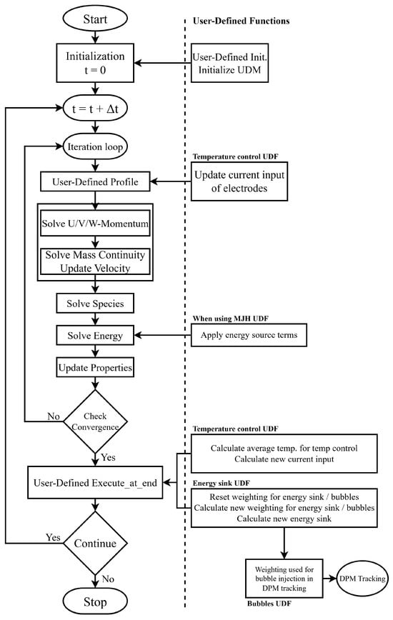
Figure 5.
Solution procedure for a pressure-based segregated solver, including UDFs. Adapted and simplified from refs. [42,43] to represent the presented model.
2.10. Convergence
The termination point for the transient simulation, thus establishing a pseudo-steady state, was determined by evaluating distinct variables within the slag layer, which represents the primary focus of this paper. These variables include the mean and maximum velocity of the slag, as well as the mean and maximum temperature of the slag. If all of these values show reasonable consistency, it is considered a pseudo-steady state.
As the termination point, a flow time of 337 s was chosen, which translates to 20,220 time steps with a time step size of 1/60 s. Depending on the hardware configuration, as different workstations were used throughout this study, the simulation required approximately one week to complete using 16 CPU cores.
Figure 6 illustrates the evolution of the mean and maximum slag velocity over the flow time, with the red line at 337 s flow time marking the termination point of the simulation. The plot shows that the mean velocity does not change substantially after around 50 s of flow time. The same is observed for the maximum velocity, although the curve is noticeably more irregular than the mean velocity. These spikes are attributed to limitations in the reporting method of ANSYS Fluent, which only captures data from the initialized cell zones. It is therefore not able to track and report the entire slag phase in the computational domain. This means, that as the slag surface deforms (see Section 3.2), gas enters into this region and the motion of the gas–slag interface contributes to artificially high velocity readings. To partially mitigate this limitation and to better visualize the pseudo-steady state of the maximum velocity of the slag, a polynomial trendline (4th degree) is included in the plot.
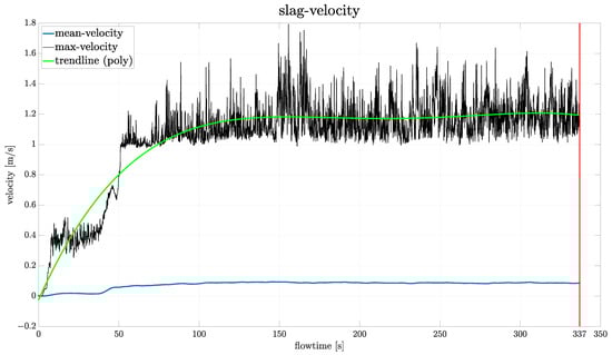
Figure 6.
Plot of the mean and maximum slag velocity over flow time. A polynomial trendline (4th degree) is fitted to the maximum velocity to illustrate pseudo-steady state behaviour. The vertical line indicates the time instant used for further evaluation. A time step size of 1/60 s was used.
Figure 7 presents the evolution of the mean and maximum slag temperature over the flow time. The mean temperature increases continuously until approximately 150 s flow time, at which point the entire slag layer nearly reaches the target temperature specified by the temperature control UDF (see Section 2.8.4). It should be noted that the zone used by the temperature control to adjust the electric current input is considerably smaller than the entire slag region that is shown in this plot. Therefore, slight deviations between the set target temperature (1630 °C) and the global mean temperature are expected. From 150 s onward, the mean temperature shows small oscillations, which are caused by the PI-control-loop (Section 2.8.4). However, these fluctuations of around 2 K at temperatures exceeding 1600 °C can be considered thermally stable. The maximum temperature shows a rapid initial increase followed by a gradual leveling off. After approximately 150 s of flow time, it remains constant, mirroring the oscillations of the mean temperature curve. Although this plot is also affected by the previously mentioned reporting limitations, the associated effects are significantly less pronounced than in the velocity data.
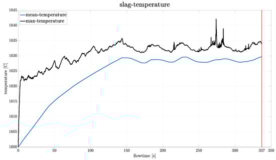
Figure 7.
Plot of the mean and maximum temperature of the slag over the flow time. The vertical line indicates the time instant used for further evaluation. A time step size of 1/60 s was used.
When examining the plots presented in (Figure 6 and Figure 7), one might question why a flow time of 337 s was chosen as the termination point, given that convergence appears to occur much earlier. The reasoning behind this decision was that the behaviour of the model was not known at this point. Therefore, the simulation time was deliberately extended to ensure that a pseudo-steady state was actually reached. In subsequent simulations, such as those conducted for the parameter study (Section 3.6), terminations were performed earlier if the model showed appropriate behaviour.
It should be noted that the results presented in Section 3 explicitly show the instantaneous state of the model at 337 s of flow time.
3. Results and Discussion
A base model was established, which incorporates all previously mentioned UDFs and explicitly solves the potential equation. The presented results refer to this base model and therefore are without the implementation of the MJH approach.
The analysis strategy was to first present and validate the results of the established base model. Due to the absence of experimental and operational data, it was not possible to undertake quantitative validation. Instead, the simulated flow, thermal behaviour, and electric results were assessed through qualitative comparison with the results reported in the available literature, thereby ensuring the physical plausibility of the model predictions.
The parameter study aims to identify controllable parameters and evaluate their influence on the mixing within the slag layer to find the optimal configuration for maximizing the phosphorus recovery efficiency.
3.1. Grid Independence Study
To assess the influence of the mesh, three different grids were simulated, consisting of approximately 190 k, 280 k, and 478 k cells. As these are transient simulations, a point of termination must be defined, which is discussed in detail in Section 2.10. However, due to the nature of the simulated system, fluctuations in the volume-averaged values of the velocity and temperature persist even after reaching a quasi-steady state. These variations are also visible in Figure 6 and Figure 7, which show the velocity with respect to the temperature of the slag over time.
To evaluate the different grids, the time-averaged and volume-averaged velocity magnitude and the corresponding standard deviation were used. A summary of these values is provided in Table 2. The temperature cannot be used for this evaluation, as it is controlled by a temperature control loop (see Section 2.8.4). The 190 k and 478 k mesh yield very similar results in both the time average and the standard deviation of the volume-averaged velocity magnitude. Using the 478 k mesh as reference, which was ultimately selected for further simulations, the difference is only 0.9% for the time average and 4.2% for the standard deviation. Interestingly, the results of the 280 k mesh deviate more than those from the 190 k mesh, with the differences being 9.4% for the time average and 2.5% for the standard deviation. This deviation likely arises from the various UDFs implemented into the model (see Section 2.8 and subsequent sections), which dynamically affect the evolution of the system as they are dynamically applied. Furthermore, since some of these UDFs are cell-based, the used mesh is expected to have a certain, but minor influence. Considering these challenges in achieving perfect grid independence, the obtained results were considered to be sufficiently constant, and the 478 k mesh was selected for subsequent simulations. Further refinement to a mesh size above 480 k cells was not pursued due to computational cost constraints.
Table 2.
Time avg. of the volume avg. velocity magnitude and corresponding standard deviation of different grids.
3.2. Slag Velocity Distribution: Influence of Bubbles and Convection
This study employs a novel and advanced CFD model that explicitly accounts for chemical reactions, gas generation, and Joule-heating, enabling a more comprehensive representation of the Submerged Arc Furnace’s behaviour. In particular, bubbles generated by the reduction reaction have a pronounced effect on the overall system dynamics and are thus decisive for interpreting later results. Therefore, the results concerning the bubble and velocity distributions are presented first, as these strongly influence and support the understanding of the subsequent findings.
Figure 8 shows the bubble distribution and their vertical velocity in Section 2.10, established as pseudo-steady state, which was reached after a flow time of 337 s. The bubble tracking is terminated once the bubbles transition from the slag into the gas phase. Consequently, the bubble distribution also reflects the deformation of the slag surface. This deformation of the top slag layer is portrayed in Figure 9 and results directly from the vertical bubble velocity that imparts momentum to the slag. The large quantity of bubbles rising in the direct vicinity of the electrodes due to the chemical reaction leads to a significant bulging of the slag surface due to the inertia of the rising slag, approximately 50 mm higher than the initialized level (visualized by the black outline; see Figure 9). Consequently, the slag height decreases in regions further away from the electrodes to conserve the total volume. The deformation of the slag surface has no implications on furnace operation, as it is small compared to the distance to the lid. This bulging of the slag is also seen in simulations of steel ladles and bubble columns [24,25].
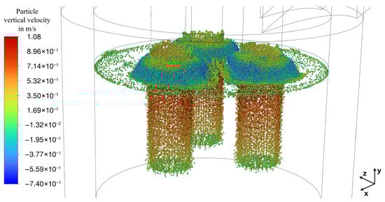
Figure 8.
Bubbles’ vertical velocity at steady state (337 s of flow time).
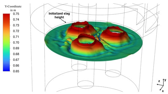
Figure 9.
Iso-clip of the slag top layer where the volume fraction of slag at steady state (337 s flow time).
The bubbles also create voids that are the primary cause of the so-called arcing phenomenon, which was observed by Sheng et al. [14,20]. This phenomenon is discussed in greater detail, explaining why it was neglected in the present study in Section 2.7. Furthermore, it should be emphasized again that, according to the work of Liu et al. [24], the mass flow rate of the bubbles has a much greater influence on slag mixing than bubble diameter.
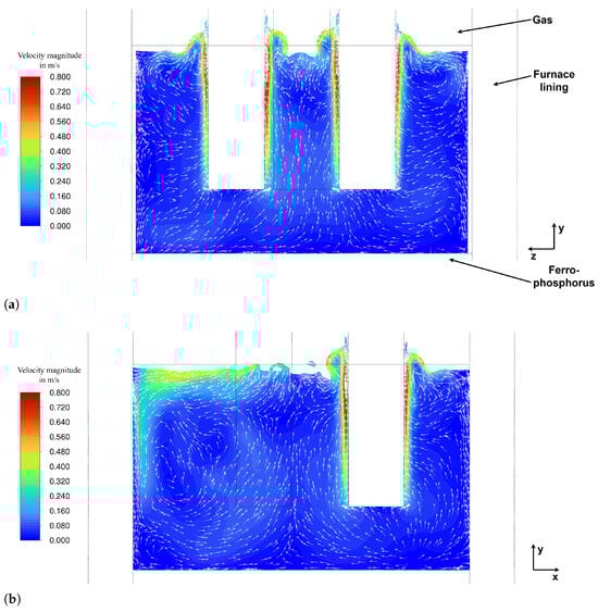
The analysis of bubble influence on flow and mixing reveals that the bubbles accelerate along the electrodes, transferring part of their momentum to the slag before escaping at the gas–slag interface. The terminal velocity of the bubbles is approximately 0.95–1.08 m/s, leading to a maximum slag velocity of approximately 0.9–1.0 m/s in the immediate vicinity of the electrodes, portrayed in Figure 10a,b. The slip velocity between the slag and the bubbles was found to be between 0.08 m/s and 0.14 m/s.
The presented model exclusively considers bubbles. Owing to their higher mass flow rate (≈70% , ≈30% ) and lower density compared to , their contribution to bubble-driven mixing is dominant. However, neglecting bubbles can result in an underestimation of the total gas mass flow rate and, consequently, of the bubble-induced momentum transfer. Including bubbles would therefore further enhance upward momentum and slag mixing and the present results should be interpreted as a lower bound for bubble-induced mixing. Since constitutes the majority of the generated gas and is denser than (density ratio ), the influence of on the flow field is expected to be secondary relative to .
The velocity field of the slag in cutting plane A (see Figure 2) is shown in Figure 10a. The overall flow field reveals an upward movement of slag in the vicinity of the electrodes. This is caused by two mechanisms:
- Natural buoyancy— slag heats up near the electrodes, which reduces its density and therefore causes it to rise.
- Bubbles—the bubbles, which have a much lower density than the slag, ascend and impart a substantial amount of their momentum to the surrounding slag, increasing the velocities in the bubble-rich regions.
This upward flow of the slag transitions into a radial outward flow near the slag surface, followed by downward flow along the furnace wall as the slag cools down slightly.
Figure 10b illustrates the flow field in cutting plane B (see Figure 2), clearly showing the formation of vortices characterized by an upward flow between the electrodes and a downward flow near the walls. The strong outward flow observed in the left half of Figure 10b at the slag surface is caused by the interaction between neighbouring electrodes, as the flow field is shown in the region between two electrodes. Therefore, the outward flow generated by each electrode converges and combines in this area, resulting in an intensified flow towards the furnace wall. However, a more detailed inspection of the flow field reveals a generally complex flow behaviour, as three-dimensional effects play a significant role in the presented model.
Overall, the bubbles play a dominant role in driving circulation and mixing throughout the slag layer, whereas natural convection contributes only secondarily in the presented model. Early simulations that considered only natural convection substantially underestimated the slag velocity distribution, highlighting the crucial role of bubbles in bath mixing. These findings are consistent with the observations of Bezuidenhout et al. [19,23] and Sheng et al. [20], who also highlighted the significance of bubbles in terms of bath mixing. This considerable momentum imparted by the bubbles consequently results in more pronounced interfacial deformation, portrayed in Figure 9, in comparison to previous studies. Generally, the slag is considered well mixed, which favours a high phosphorous recovery efficiency as it ensures that unreduced slag, containing the elements required for the reduction reaction, is present in the reaction zone. Additionally, a relatively uniform temperature distribution is favoured by the heavy mixing. The region where mixing is most limited is found to be at the bottom of the slag layer, near the furnace wall.
To illustrate the complex flow behaviour mentioned before, Figure 11 shows the pathlines in the slag layer, coloured by vertical velocity, where red indicates an upward flow and blue a downward flow. It can be seen that in regions where the electrodes are positioned closest to the wall, the flow near the wall is actually directed upward, a behaviour also visible in Figure 10a,b. This phenomenon is likely caused by several factors, one of which is the presence of significant 3D-flow effects. Additionally, it predominantly occurs in regions where the electrodes are closest to the wall, suggesting that the slightly elevated Joule-heating in these areas—due to the reduced distance to the wall—contributes to the observed behaviour. Furthermore, the furnace walls are not water-cooled, in contrast to various other studies [19,20,23], which reflects the actual furnace design. The absence of intensive wall cooling reduces downward wall-adjacent flow and is therefore believed to enable the observed upward motion along the wall. While the numerical framework supports the inclusion of water-cooled walls if required, their introduction would intensify downward wall-adjacent flow due to enhanced cooling, while simultaneously increasing heat losses and reducing thermal efficiency. As mentioned previously, the overall flow field remains predominantly bubble driven.
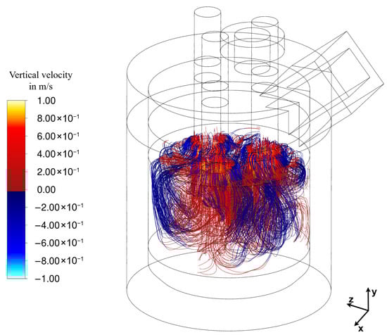
Figure 11.
Pathlines and vertical velocity at steady state (337 s flow time) in the slag-layer (red—upward flow; blue—downward flow).
3.3. Electric Results
The electric results are only available when the potential equation described in Section 2.7 is solved. These results provide insight into the major heating mechanism of the SAF, which are described and discussed in the following subsections.
3.3.1. Electric Potential Distribution
The electric potential along the vertical cross-section A (Figure 2) is illustrated in Figure 12. At the displayed time, the right electrode is in an input state, while the left electrode is receiving the current. The outer boundary of the furnace is grounded, as mentioned in Section 2.3. The observed distortion of the electric field near the gas–slag interface is attributed to the non-uniform slag surface (Figure 9), which is deformed due to bubble formation and upward slag flow (Figure 10). Aside from this localized deviation, the behaviour aligns with the observations of Bezuidenhout et al. [19,23] and Sheng et al. [14,20].
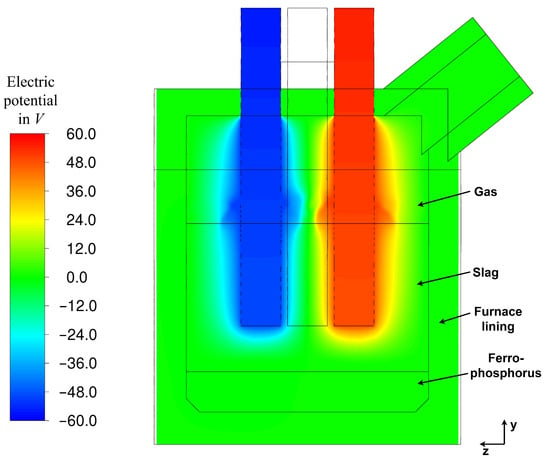
Figure 12.
Electric potential at steady state (337 s of flow time) along cutting plane A (Figure 2).
3.3.2. Current Density Distribution
The current density distribution, shown in Figure 13, follows the potential distribution (Figure 12). As expected, current flows from the input electrode to the output electrode, as well as to and from the grounded outer boundary, depending on the electrode input state. Due to the very low electrical conductivity of the gas phase, current flow within it, though illustrated, is negligible—in the order of to A/m2—meaning that nearly all current is conducted through the slag and ferrophosphorus layers.
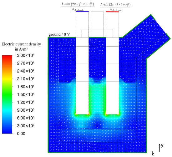
Figure 13.
Current density at steady state (337 s of flow time) along cutting plane A (Figure 2).
Closer inspection of the current density field reveals three distinct current pathways. The first is a direct path between the input and output electrodes. The second pathway leads from the inputting electrode through the slag to the ferrophosphorus layer and from there to the outputting electrode. The third pathway is seen to be a radial flow of current either to or from the grounded outer boundary, depending on the electrode’s input state.
These current paths are consistent with observations from other studies [15,19,21,23]. However, the model presented here exhibits a stronger direct current flow between the electrodes, which can be attributed to the smaller electrode spacing compared to other published results. Additionally, the deformation of the slag surface (Figure 9), caused by the bubbles and upward slag flow, is clearly visible and impacts the current density distribution, highlighting the influence of multiphase flow on the electrical behaviour. The current distribution, together with the electrical conductivity , also directly correlates with Joule-heating (Figure 14).
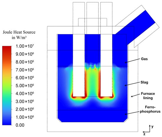
Figure 14.
Joule-heating at steady state (337 s of flow time) along cutting plane A (Figure 2).
3.3.3. Power Distribution (Joule-Heating)
The Joule-heating distribution, shown in Figure 14, closely follows the current density , as Joule-heating is proportional to . The highest heat generation occurs in the immediate vicinity of and between the electrodes, which is consistent with findings from other studies [15,19,20,23].
Although a significant portion of the current passes through the ferrophosphorus layer (illustrated in Figure 13), only minimal heat is generated within. This is due to the high electrical conductivity of the ferrophosphorus layer compared to the slag, which reduces the local resistive heating. The local peaks observed at the top of the slag layer between the electrodes are attributed to the interpolation of electrical conductivity at the deformed VOF interface (Figure 9) between slag and gas. This effect arises from numerically blending the material properties in the interface region. Regardless of this effect, almost the entire heat is generated within the slag.
All the electric results are linked via the potential equation, causing the system to heat up through Joule heating. The increased temperature then facilitates the onset of the reaction, whereby a higher temperature causes a higher reaction rate and therefore generates more bubbles but also leads to a higher energy sink. The resulting bubbles and natural buoyancy subsequently affect the mixing.
3.4. Temperature Distribution
The temperature distribution at pseudo-steady state (337 s of flow time) along various cutting planes is illustrated in Figure 15, where the contour lines for the fluids are presented in a narrow scale for better visibility. The solid bodies are presented in grayscale and are capped to better present the temperature gradients. Note that the temperature at the top of the electrodes is far below 1550 °C as they are actively cooled. Figure 15a depicts the temperature field along cutting plane A (Figure 2), revealing a largely uniform temperature distribution in both the gas and slag layers. The target temperature of 1630 °C—defined by the temperature control strategy described in Section 2.8.4—was effectively reached throughout the gas and slag domains. This highlights the effectiveness of the temperature control loop. The simulation was initialized at 1600 °C and stopped after a flow time of 337 s, using a time step size of 1/60 s.
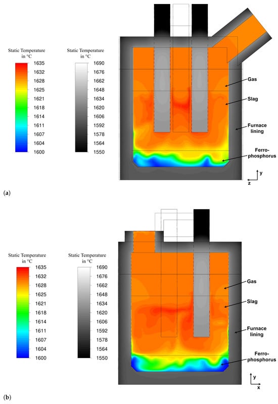
Slightly elevated temperatures are observed in the vicinity of and between the electrodes, which corresponds to the Joule-heating distribution shown in Figure 14. However, due to heavy mixing and thermal conduction, the temperature contour lines in the slag layer are more diffused than one would expect based solely on the Joule-heating profile (Figure 14). Closer to the walls, the temperature decreases slightly according to the imposed boundary conditions (see Section 2.3). In the region near the ferrophosphorus interface, a thin, cooler layer is visible at the wall. This reduced temperature results from limited bath mixing in these areas, making thermal conduction the dominant heat transport mechanism.
Investigating Figure 15b, which illustrates the temperature along cutting plane B (Figure 2), yields largely the same observations as those from Figure 15a. The elevated temperature near the velocity inlet is attributed to the higher specified inlet temperature at the inlet boundary. Additionally, it can be observed that the region of increased temperature extends slightly beyond the radius on which the electrodes are positioned. When correlating the velocity distribution (Figure 10a,b) with the temperature distribution, it appears that the regions of elevated temperature are not located directly at the surface of the slag layer, but rather slightly beneath it, corresponding to zones of lower velocity magnitude. Compared to other studies [15,19,20,23], the temperature distribution in the presented model is noticeably more uniform. This deviation from the literature is likely attributable to the significantly smaller furnace size, the absence of water-cooled walls, the inclusion of radiative heat transfer (which is not consistently considered in other studies), and heavier mixing within the slag layer (see Section 3.2).
3.5. Implications of the Results on Phosphorus Recovery
The resulting velocity field (Figure 10) directly governs the residence time and renewal rate of slag in the reaction zone. Enhanced mixing increases the probability that unreduced slag repeatedly enters this region, thereby promoting phosphorus recovery, whereas weakly mixed or stagnant regions reduce the recovery. In addition, the electrical potential and current density fields (Figure 12 and Figure 13) are coupled through the potential equation Equation (12) and give rise to volumetric Joule-heating (Figure 14), which represents the dominant internal heat source within the slag. The associated temperature gradients induce buoyancy forces and contribute to natural convection, while the elevated temperatures enable the onset of the reduction reaction and influence local reaction rates.
The reaction itself introduces an energy sink (Section 2.8.2) associated with reaction enthalpy and bubble generation (Section 2.8.3). The formation of gas bubbles further enhances mixing, particularly within the reaction region, but also promotes global circulation throughout the slag bath. Although bubble formation and dynamics are simplified in the present model, their coupling with the flow and temperature fields is captured, resulting in a relatively uniform temperature distribution (Figure 15) facilitated by the enhanced mixing. The region where mixing remains most limited is located near the bottom of the slag layer close to the furnace wall.
3.6. Parameter Study
The model was modified to investigate the influence of varying distances between the electrodes and the impact of different slag viscosities on the flow field. The influence of different immersion depths was already investigated in the literature [15,19,23].
For the real system, it is most important that good mixing of the slag is ensured, as this leads to the highest phosphorus recovery efficiency. To maximise mixing, the influence of different parameters has to be investigated. Therefore a parameter study was conducted where both the distance between the electrodes and slag viscosity were varied to investigate their impact on the flow behaviour and temperature distribution within the refiner. The base case features electrodes positioned on a circle with a radius of R = 200 mm (Figure 2) and a slag viscosity of 0.3 Pa·s. The results previously presented correspond to this base case. Starting from this configuration, the slag viscosity was reduced to 0.1 Pa·s resp. 0.2 Pa·s to examine the influence of lower viscosity on system behaviour.
This variation in viscosity was investigated as exact measurements are not possible and the viscosity might vary between different batches, as it is dependent on the slag composition. In a second case, the electrode placement radius was reduced to R = 150 mm (Figure 2), and simulations were conducted for all three slag viscosities (0.3 Pa·s, 0.2 Pa·s, 0.1 Pa·s). This resulted in, thus far, a total of six scenarios, enabling a comparative analysis of how electrode proximity and slag viscosity affect the flow and temperature behaviour. For the evaluation, cell values were used, with volume-averaged quantities computed for mean values. Only cells with a slag volume fraction were considered to avoid including the dynamic interface behaviour. A summary of the results is provided in Table 3. These results are time averaged, as due to the nature of the simulated system, fluctuations occur, which was also discussed in Section 3.1.
Table 3.
Summary of time-averaged maximum and volume-average values of velocity and temperature for different slag viscosities and electrode placement radii R (see Figure 2).
Analyzing the results, it is evident that reducing slag viscosity within the same electrode configuration leads to an increase in both mean and maximum velocity. This is expected behaviour. For the base case with a viscosity of 0.3 Pa·s, the volume-averaged velocity magnitude in the slag phase is 0.088 m/s, while the maximum velocity magnitude is 1.013 m/s. When changing the viscosity to 0.1 Pa·s, the average increases to 0.166 m/s and the maximum to 1.309 m/s. Comparing the different viscosities for the 150 mm case also yields an increase from 0.093 m/s to 0.124 m/s for the average velocity and from 1.032 m/s to 1.210 m/s for the maximum velocity. The results for a viscosity of 0.2 Pa·s are in both cases placed between these. The increase in maximum velocity from 0.3 Pa·s to 0.1 Pa·s is 29.3%, while the increase from 0.3 Pa·s to 0.2 Pa·s is 14.6%. This shows that the result for 0.2 Pa·s is almost exactly halfway between the other two. A similar trend appears in the volume avg. velocity, although the values are not as symmetrically spaced. Here, the result increases by 87.4% from 0.3 to 0.1 Pa·s and by 37.6% from 0.3 to 0.2 Pa·s. The same behaviour is seen when analysing the results from the 150 mm case.
However, when comparing cases with different electrode distances but same viscosity, no clear trend emerges. This is likely due to the influence of the temperature control loop (Section 2.8.4), keeping both models at approximately the same point of operation with only minor variations. It is also suspected that the Joule-heating—which, in the 150 mm case, is more concentrated near the center of the SAF and leads to a higher average velocity between the electrodes—is counterbalanced by lower velocities occurring near the walls. This can therefore be considered a geometric effect. Table 3 therefore shows that lowering the viscosity within the same case leads to higher velocities and consequently to a better mixing of the slag. This is valuable information as the viscosity can be adjusted with additives. In contrast, reducing the distance between the electrodes does not necessarily increase the velocity and thus the mixing, as the effect of the increased Joule-heating on the flow field between the electrodes is mitigated by the temperature control loop and geometric effects. The difference in temperature, both maximum and volume average, are minimal in all cases, highlighting the effectiveness of the temperature control loop.
In summary, altering the viscosity of the slag has a definitive impact on the velocity and therefore the mixing, while changing the electrode placement radius shows no clear correlation. With respect to maximizing phosphorus recovery efficiency, the optimal configuration corresponds to the base case with R = 200 mm (Figure 2) and the lowest considered viscosity of 0.1 Pa·s. This configuration yields the highest maximum and average slag velocities, thereby promoting the most effective mixing.
3.7. Results Using the Mean-Joule-Heating Approach
The results presented so far, as stated at the beginning of Section 3, are from the model that solves the potential equation (Section 2.7). However, since a novel approach to reduce simulation time is introduced in Section 2.8.5, the corresponding results are also presented here. The Mean-Joule-heating (MJH) method offers a simulation speed-up of up to 300% at the cost of some accuracy. In this approach, the Joule-heating (Section 3.3.3) is applied as a source term, using values from a previous simulation that are scaled via the temperature control loop (Section 2.8.4) to also account for furnace control. All other UDFs are identical in both approaches.
Figure 16 shows the MJH after 60 s flow time with A used in Equation (14) along cutting plane A (Figure 2). These mean values are exported as a CSV file and subsequently used by a UDF to assign each cell its corresponding Joule-heating as an additional source term. This approach eliminates the need to solve the potential equation directly, significantly reducing the overall simulation time. A more detailed discussion of this approach is found in Section 2.8.5.
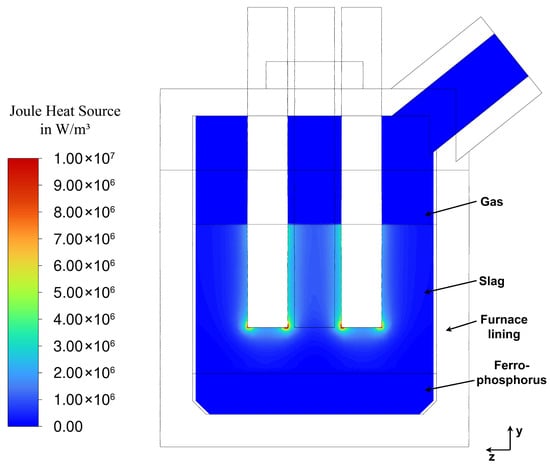
Figure 16.
Mean-Joule-heating after 60 s flow time with A along cutting plane A (Figure 2).
Figure 17 compares the results of the potential model with those obtained using the MJH approach. Figure 17a shows the velocity magnitude in the slag layer along cutting plane A (Figure 2). The MJH model agrees well with the potential model, with only minor deviations in the wall-adjacent vortices, while the overall flow pattern and velocity remain similar.
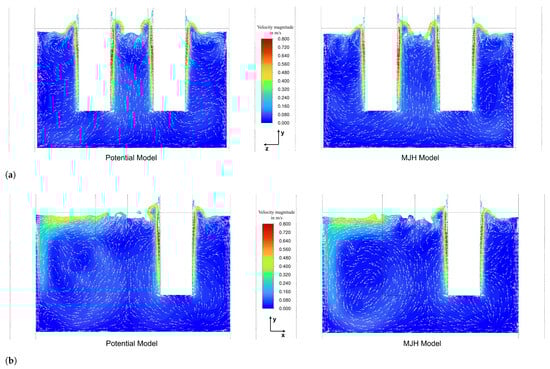
Figure 17.
(a) Comparison of the velocity magnitude in the slag layer between the potential model and the MJH model at 337 s flow time along cutting plane A (Figure 2). (b) Comparison of the velocity magnitude in the slag layer between the potential model and the MJH model at 337 s flow time along cutting plane B (Figure 2).
Figure 17b leads to the same conclusion, showing the most noticeable differences in the flow field near the wall, while the general flow of both models is similar.
Considering the dynamic nature of the system, as well as the influence of UDFs and the different simulation approaches on the transient evolution (also discussed in Section 3.1), the results of both models can be regarded as being in good overall agreement.
Table 4 gives a summary of the time-averaged values obtained by the two different simulation approaches, with the same evaluation procedure as in the parameter study (Section 3.6). The MJH model only shows a difference of 3.8% for the maximum velocity and 2.0% for the average velocity, while the difference in the temperature is only minimal, as both models use the temperature control UDF.
Table 4.
Summary of time-averaged maximum and volume-average values of velocity and temperature of the potential model and the MJH model.
Overall, the MJH approach significantly reduces simulation time while still delivering sufficiently accurate results. It is therefore well suited for applications where fast results are required and the highest level of accuracy is not critical, such as preliminary parameter studies. Additionally, it should be noted that the actual acceleration of the simulation by the MJH model is also heavily dependent on the used model and its complexity. The model, which is presented, was accelerated by approximately 100%, while earlier, less complex models showed an acceleration of up to 300%.
4. Conclusions and Outlook
A comprehensive CFD model of a Submerged Arc Furnace (SAF) for slag reduction has been developed. It minimizes the computational expense through approximating complex phenomena by the use of multiple UDFs and demonstrates further possibilities of numerical cost reduction, such as the Mean-Joule-heating (MJH) approach. The model captures multiple key phenomena, including multiphase flow, bubble generation due to chemical reactions, energy sink coupling, the solution of the potential equation and associated Joule-heating, as well as simulating the furnace control.
The dynamic energy sink and bubble generation are modelled as functions of local cell temperature and volume, representing their direct dependence on the chemical reaction. The influence of electrode distance and slag viscosity on system behaviour was also investigated. Furthermore, a novel MJH approach was suggested, enabling the simulation to bypass the explicit solution of the potential equation and accelerating the simulation by a factor of up to 300% while still capturing the essential system behaviour.
The current density revealed three main pathways, one from the inputting electrode through the slag and the highly conductive ferrophosphorus layer to the outputting electrode, a second pathway occurring directly between the electrodes, and the third between the electrodes and the grounded walls. As expected, Joule-heating closely followed the current density distribution, with the highest heat generation occurring in the immediate vicinity of the electrodes.
The resulting temperature field showed a largely uniform temperature within the slag layer, closely matching the target value set by the temperature control loop (±2 K) and highlighting its effectiveness. This uniformity in temperature can additionally be attributed to strong bubble driven mixing in the slag. In contrast, the temperature distribution in the ferrophosphorus layer was primarily dependent on thermal conduction, due to limited motion and minimal Joule-heating.
It was revealed that bubble generation has a significant impact on the velocity distribution, especially in the modelled process, where the bubble generation is not limited to the electrode surface, and the compact geometry of the refiner amplifies their influence on the whole flow field. The flow field generally showed the formation of vortices, where the slag generally rises near the electrodes and descends along the wall. The highest velocities of 0.9–1.0 m/s were found in the vicinity of the electrodes. However, the simulation revealed a more complex flow pattern within the slag-layer, where 3D-flow effects and the proximity of the electrodes to the wall play a significant role. Additionally, it was shown that the momentum of the rising slag and bubbles has a significant impact on the deformation of the slag interface. Leading to a deformation of approximately 50 mm compared to the initialized height and caused by the inertia of the rising slag.
Slag viscosity was found to directly influence both the maximum and mean velocities while having no significant effect on the temperature. In contrast, changing the electrode distance showed no clear correlation, likely due to the temperature control loop maintaining a constant operating point.
Overall, the model incorporates key physical phenomena that have been strongly simplified or overlooked in the prior literature while maintaining computational efficiency. It provides a solid foundation for further improvements and investigations. Initial tests transferring the mass, momentum and energy of the bubbles to the gas phase, to simulate the gas flow, have shown promising results.
Author Contributions
Conceptualization, D.W. and B.O.; methodology, D.W. and B.O.; software, D.W.; validation, D.W.; formal analysis, D.W.; investigation, D.W.; resources, B.O., R.P. and V.M.; data curation, D.W.; writing—original draft preparation, D.W.; writing—review and editing, D.W. and B.O.; visualization, D.W.; supervision, C.H.; project administration, C.H.; funding acquisition, C.H. All authors have read and agreed to the published version of the manuscript.
Funding
This project has received funding from the European Union’s Horizon 2020 research and innovation programme under grant agreement No. 958267.
Data Availability Statement
Data will be made available on request.
Acknowledgments
During the preparation of this manuscript/study, the authors used ChatGPT and DeepL Write for the purposes of improving the readability and language of the manuscript. The authors have reviewed and edited the output and take full responsibility for the content of this publication.
Conflicts of Interest
Author Valentin Mally was employed by the “ARP” Aufbereitung, Recycling und Prüftechnik Gesellschaft m.b.H. The remaining authors declare that the research was conducted in the absence of any commercial or financial relationships that could be construed as a potential conflict of interest.
Abbreviations
The following abbreviations are used in this manuscript:
| AC | Alternating Current |
| BC | Boundary Condition |
| CFD | Computational Fluid Dynamics |
| CSV | Comma-separated Values |
| DO | Discrete Ordinates |
| DPM | Discrete Phase Model |
| EAF | Electric Arc Furnace |
| FVM | Finite Volume Method |
| MJH | Mean-Joule-heating |
| PISO | Pressure-Implicit with Splitting of Operators |
| SAF | Submerged Arc Furnace |
| UDF | User-Defined Function |
| UDM | User-Defined Memory |
| VOF | Volume of Fluid |
References
- McDowell, R.W.; Pletnyakov, P.; Haygarth, P.M. Phosphorus applications adjusted to optimal crop yields can help sustain global phosphorus reserves. Nat. Food 2024, 5, 332–339. [Google Scholar] [CrossRef]
- Yu, M.; Gao, Z.; Xie, W.; Shi, X.; Zhang, O.; Shen, Z.; Fang, L.; Ren, M.; Sun, J. A novel strategy utilizing oxidation states of phosphorus for designing efficient phosphorus-containing flame retardants and its performance in epoxy resins. Polym. Degrad. Stab. 2024, 230, 111016. [Google Scholar] [CrossRef]
- European Food Safety Authority (EFSA). Assessment of One Published Review on Health Risks Associated with Phosphate Additives in Food. EFSA J. 2013, 11, 3444. [Google Scholar] [CrossRef]
- Atienza-Martínez, M.; Gea, G.; Arauzo, J.; Kersten, S.R.; Kootstra, A.M.J. Phosphorus recovery from sewage sludge char ash. Biomass Bioenergy 2014, 65, 42–50. [Google Scholar] [CrossRef]
- Ortner, B.; Schmidberger, C.; Gerhardter, H.; Prieler, R.; Schröttner, H.; Hochenauer, C. Application of computationally inexpensive CFD model in steady-state and transient simulations of pulverized sewage sludge combustion. Adv. Powder Technol. 2023, 34, 104260. [Google Scholar] [CrossRef]
- Xu, Y.; Zhang, L.; Chen, J.; Liu, T.; Li, N.; Xu, J.; Yin, W.; Li, D.; Zhang, Y.; Zhou, X. Phosphorus recovery from sewage sludge ash (SSA): An integrated technical, environmental and economic assessment of wet-chemical and thermochemical methods. J. Environ. Manag. 2023, 344, 118691. [Google Scholar] [CrossRef] [PubMed]
- Ortner, B.; Schmidberger, C.; Prieler, R.; Mally, V.; Hochenauer, C. Analysis of the shear-driven flow in a scale model of a phase separator: Validation of a coupled CFD approach using experimental data from a physical model. Int. J. Multiph. Flow 2024, 177, 104852. [Google Scholar] [CrossRef]
- Ortner, B.; Peham, L.; Schmidberger, C.; Prieler, R.; Hochenauer, C. CFD modeling of sewage sludge combustion in an experimental entrained flow reactor with integrated slag flow dynamics. Appl. Therm. Eng. 2025, 267, 125779. [Google Scholar] [CrossRef]
- Askarizadeh, H.; Lotfollahzadeh, A.; Wolfersdorf, C.; Pielsticker, S.; Kneer, R. An equilibrium calculation tool with development potential for predicting phosphorus recovery from sewage sludge in entrained-flow gasifiers. Chem. Eng. Res. Des. 2023, 197, 53–64. [Google Scholar] [CrossRef]
- Scheepers, E.; Yang, Y.; Adema, A.T.; Boom, R.; Reuter, M.A. Process Modeling and Optimization of a Submerged Arc Furnace for Phosphorus Production. Metall. Mater. Trans. B 2010, 41, 990–1005. [Google Scholar] [CrossRef]
- Piro, N.A.; Figueroa, J.S.; Mckellar, J.T.; Cummins, C.C. Triple-Bond Reactivity of Diphosphorus Molecules. Science 2006, 313, 1276–1279. [Google Scholar] [CrossRef]
- Kotze, A.; Messina, D.; Cryns, Y.; Nagels, E.; Arnout, S. Thermochemical evaluation of elemental phosphorus recovery from sewage sludge. J. South. Afr. Inst. Min. Metall. 2025, 125, 501–508. [Google Scholar] [CrossRef]
- Jones, P.L.; Taylor, S.; Nakai, S.; Jennings, J. Electroheat and Materials Processing. In Electrical Engineer’s Reference Book; Elsevier: Amsterdam, The Netherlands, 2003; pp. 9-1, 9-3–9-38. [Google Scholar] [CrossRef]
- Sheng, Y.Y.; Irons, G.A.; Tisdale, D.G. Transport phenomena in electric smelting of nickel matte: Part I. Electric potential distribution. Metall. Mater. Trans. B 1998, 29, 77–83. [Google Scholar] [CrossRef]
- Karalis, K.T.; Karkalos, N.; Cheimarios, N.; Antipas, G.; Xenidis, A.; Boudouvis, A.G. A CFD analysis of slag properties, electrode shape and immersion depth effects on electric submerged arc furnace heating in ferronickel processing. Appl. Math. Model. 2016, 40, 9052–9066. [Google Scholar] [CrossRef]
- Vångö, M.; Pirker, S.; Lichtenegger, T. Unresolved CFD–DEM modeling of multiphase flow in densely packed particle beds. Appl. Math. Model. 2018, 56, 501–516. [Google Scholar] [CrossRef]
- Barral, P.; Pérez-Pérez, L.J.; Quintela, P. Transient thermal response with nonlocal radiation of a blast furnace main trough. Appl. Math. Model. 2022, 105, 197–225. [Google Scholar] [CrossRef]
- Bermúdez, A.; Crego, O.; Ferrín, J.L.; García, B.; Gómez, D.; Martínez, I.; Pérez-Pérez, L.J.; Salgado, P. Multiphysics simulation of slag melting in an induction furnace for sustainable silicon production. Appl. Math. Model. 2025, 145, 116107. [Google Scholar] [CrossRef]
- Bezuidenhout, J.J.; Eksteen, J.J.; Bradshaw, S.M. Computational fluid dynamic modelling of an electric furnace used in the smelting of PGM containing concentrates. Miner. Eng. 2009, 22, 995–1006. [Google Scholar] [CrossRef]
- Sheng, Y.Y.; Irons, G.A.; Tisdale, D.G. Transport phenomena in electric smelting of nickel matte: Part II. Mathematical modeling. Metall. Mater. Trans. B 1998, 29, 85–94. [Google Scholar] [CrossRef]
- Jardy, A.; Ablitzer, D.; Wadier, J.F. Magnetohydronamic and thermal behavior of electroslag remelting slags. Metall. Trans. B 1991, 22, 111–120. [Google Scholar] [CrossRef]
- Choudhary, M.; Szekely, J. Some General Characteristics of Heat and Fluid Flow Phenomena in Electric Melting and Smelting Operation. J. Min. Metall. Sect. B Metall. 1981, 90, 164. [Google Scholar]
- Bezuidenhout, J.J.; Eksteen, J.J.; Bradshaw, S.M. CFD modelling of molten matte and slag flows in a circular three-phase smelting furnace. Prog. Comput. Fluid Dyn. Int. J. 2009, 9, 316. [Google Scholar] [CrossRef]
- Liu, W.; Lee, J.; Guo, X.; Silaen, A.K.; Zhou, C.Q. Argon Bubble Coalescence and Breakup in a Steel Ladle with Bottom Plugs. Steel Res. Int. 2019, 90, 1800396. [Google Scholar] [CrossRef]
- Fletcher, D.F.; McClure, D.D.; Kavanagh, J.M.; Barton, G.W. CFD simulation of industrial bubble columns: Numerical challenges and model validation successes. Appl. Math. Model. 2017, 44, 25–42. [Google Scholar] [CrossRef]
- Wang, H.; Jia, X.; Wang, X.; Zhou, Z.; Wen, J.; Zhang, J. CFD modeling of hydrodynamic characteristics of a gas–liquid two-phase stirred tank. Appl. Math. Model. 2014, 38, 63–92. [Google Scholar] [CrossRef]
- Jønck, K.M. CFD Modelling of Melting Cyclones for Stone Wool Production. Ph.D. Thesis, Technical University of Denmark, Kgs. Lyngby, Denmark, 2021. [Google Scholar]
- SGL Carbon SE. SIGRAFINE® HLM Datasheet; SGL Carbon SE: Wiesbaden, Germany, 2025; Available online: https://www.sglcarbon.com/pdf/SGL-Datasheet-SIGRAFINE-HLM-EN.pdf (accessed on 5 June 2025).
- Entegris POCO Materials. Graphite Properties and Characteristics; Entegris POCO Materials: Billerica, MA, USA, 2025. Available online: https://poco.entegris.com/content/dam/poco/resources/reference-materials/brochures/brochure-graphite-properties-and-characteristics-11043.pdf (accessed on 5 June 2025).
- Yin, Y.; Zhai, K.; Zhang, B.; Zhai, S. Electrical Resistivity of Iron Phosphides at High–Pressure and High–Temperature Conditions With Implications for Lunar Core’s Thermal Conductivity. J. Geophys. Res. Solid Earth 2019, 124, 5544–5556. [Google Scholar] [CrossRef]
- Vargas, S.; Frandsen, F.J.; Dam-Johansen, K. Rheological properties of high-temperature melts of coal ashes and other silicates. Prog. Energy Combust. Sci. 2001, 27, 237–429. [Google Scholar] [CrossRef]
- Patankar, S.V. Numerical Heat Transfer and Fluid Flow; CRC Press: Boca Raton, FL, USA, 2018. [Google Scholar] [CrossRef]
- ANSYS Inc. ANSYS Fluent Theory Guide (Release 2024 R1); ANSYS Inc.: Canonsburg, PA, USA, 2024. [Google Scholar]
- Michaelides, E.E.; Crowe, C.T.; Schwarzkopf, J.D. Multiphase Flow Handbook; CRC Press: Boca Raton, FL, USA, 2016. [Google Scholar] [CrossRef]
- Safarian, J.; Tangstad, M. Wettability of Silicon Carbide by CaO-SiO2 Slags. Metall. Mater. Trans. B 2009, 40, 920–928. [Google Scholar] [CrossRef]
- Sundström, A.W.; Eksteen, J.; Georgalli, G. A review of the physical properties of base metal mattes. J. South. Afr. Inst. Min. Metall. 2008, 108, 431–448. [Google Scholar]
- Bidi, M.; Hosseini, R.; Nobari, M. Numerical analysis of methane–air combustion considering radiation effect. Energy Convers. Manag. 2008, 49, 3634–3647. [Google Scholar] [CrossRef]
- Derby, J.; Brandon, S.; Salinger, A.G. The diffusion and P1 approximations for modeling buoyant flow of an optically thick fluid. Int. J. Heat Mass Transf. 1998, 41, 1405–1415. [Google Scholar] [CrossRef]
- Herland, E.V.; Sparta, M.; Halvorsen, S.A. Skin and Proximity Effects in Electrodes and Furnace Shells. Metall. Mater. Trans. B 2019, 50, 2884–2897. [Google Scholar] [CrossRef]
- ANSYS Inc. ANSYS Fluent User Guide (Release 2024 R1); ANSYS Inc.: Canonsburg, PA, USA, 2024. [Google Scholar]
- Tas-Koehler, S.; Liao, Y.; Hampel, U. A critical analysis of drag force modelling for disperse gas-liquid flow in a pipe with an obstacle. Chem. Eng. Sci. 2021, 246, 117007. [Google Scholar] [CrossRef]
- ANSYS Inc. ANSYS Fluent Customization Manual (Release 2024 R1); ANSYS Inc.: Canonsburg, PA, USA, 2024. [Google Scholar]
- Wu, M.; Ludwig, A.; Kharicha, A. Volume-Averaged Modeling of Multiphase Flow Phenomena during Alloy Solidification. Metals 2019, 9, 229. [Google Scholar] [CrossRef]
Disclaimer/Publisher’s Note: The statements, opinions and data contained in all publications are solely those of the individual author(s) and contributor(s) and not of MDPI and/or the editor(s). MDPI and/or the editor(s) disclaim responsibility for any injury to people or property resulting from any ideas, methods, instructions or products referred to in the content. |
© 2026 by the authors. Licensee MDPI, Basel, Switzerland. This article is an open access article distributed under the terms and conditions of the Creative Commons Attribution (CC BY) license.