Article

Exploiting the Flexibility and Frequency Support Capability of Grid-Forming Energy Storage: A Bi-Level Robust Planning Model Considering Uncertainties

by
Yijia Yuan
*,
Zheng Fan
,
Xirui Jiang
,
Yanan Wu
and
Chengbin Chi
National Key Laboratory of Advanced Power Transmission Technology (China Electric Power Research Institute), Beijing 102209, China
*
Author to whom correspondence should be addressed.
Processes 2026, 14(1), 90; https://doi.org/10.3390/pr14010090
Submission received: 1 December 2025 / Revised: 22 December 2025 / Accepted: 24 December 2025 / Published: 26 December 2025

Abstract

With the continuously rising penetration rate of variable renewable energy (VRE), issues related to power balance and frequency stability in power systems have become increasingly prominent. Battery energy storage systems (BESS) with grid-forming capabilities are regarded as an effective solution for providing rapid frequency support. However, the stochastic fluctuations of VRE output also lead to time-varying system inertia, which undoubtedly increases the complexity of energy storage planning. To address these problems, this study constructs a bi-level robust planning model for grid-forming energy storage considering frequency security constraints. First, a frequency response model for grid-forming BESS is established. By accurately describing the delay characteristics of different resources in frequency response, dynamic frequency security constraints (FSC) that can be embedded into the planning model are constructed. Subsequently, the study proposes an evaluation method for the spatial distribution of power system inertia, providing a basis for the optimal siting of BESS in the grid. On this basis, a bi-level robust planning model, considering VRE uncertainty, is constructed, which embeds an operational simulation model and incorporates FSC. To achieve an effective solution of the model, FSC is transformed into a second-order cone form, and a nested column-and-constraint generation (C&CG) algorithm is employed for solving. Simulation results on the modified NPCC-140 bus system verify the effectiveness of the proposed model. While reducing the total cost by 15.9%, this method effectively ensures the dynamic frequency security of the power system, improves the spatial distribution of inertia and significantly enhances the system’s ability to accommodate VRE.

1. Introduction

Motivated by the carbon peak and carbon neutrality objectives, China has witnessed continuous and rapid expansion in its variable renewable energy (VRE) capacity. By the end of 2024, the cumulative installed VRE capacity in China achieved a historic milestone of 1.45 billion kilowatts, exceeding thermal power capacity for the first time [1]. The extensive integration of VRE is shifting the power system away from a synchronous generator-centric paradigm toward one that relies on non-synchronous sources such as VRE. This evolving system structure is characterized by low inherent inertia and significant power fluctuations, introducing substantial challenges to operational security and stability [2,3]. Advanced forecasting methods, such as machine learning techniques, are being developed to better predict VRE output and mitigate its integration impact [4]. Concurrently, grid-forming capable resources, leveraging technologies like the virtual synchronous generator, can mimic the grid-connection behavior of traditional synchronous generators [5]. By proactively reacting to system frequency deviations, they deliver essential inertia support [6]. Thus, the strategic deployment of these resources represents a critical approach for mitigating the system’s inertia deficit [7]. Nevertheless, the inherent unpredictability of VRE generation causes virtual inertia to become time-varying, leading to a geographically uneven distribution of system inertia, complicating the application of conventional resource optimization techniques. Considering these new demands stemming from the swift advancement of renewable energy, there is a pressing need to investigate a robust planning methodology for diverse grid-forming resources. Such methods must account for VRE volatility and the necessity for frequency security support, thereby furnishing a methodological foundation for safeguarding frequency stability in power systems.
Research into modeling the contribution of grid-forming resources to frequency response has seen considerable advances. Concerning battery energy storage systems, studies have explored parameter optimization to strengthen frequency stability [8], utilized multi-variable inputs including frequency deviation, rate of change of frequency (RoCoF), and the state of charge (SOC) for enhanced response [9], and derived virtual inertia for combined wind-storage systems based on energy conversion principles [10]. In the domain of wind power, analyses of the coupling between doubly fed induction generator rotational inertia, speed, and frequency dynamics have led to improved farm-level power support [11], while integrated control frameworks enabling inertial support from wind turbines have been developed [12]. For photovoltaics, research has established dynamic models to elucidate their role in frequency regulation [13] and focused on adaptive virtual synchronous generator (VSG)control for better performance during power reductions [14]. A significant research gap remains, however, in understanding how the volatility of VRE output impacts the dependable provision of virtual inertia, particularly when multiple types of grid-forming resources interact. Accurately modeling the frequency support capabilities of a diverse portfolio of grid-forming resources, therefore, necessitates explicitly addressing the uncertainty inherent in power systems with high penetration of renewable energy sources (RES).
The effective planning of inertia resources is fundamental to system frequency security. Current literature presents various optimization strategies for virtual inertia planning. These include methods considering the spatial disparities in frequency response across the network [15], planning frameworks for emerging technologies such as grid-forming electro-hydrogen storage [16], and economically driven capacity optimization for hybrid PV-storage systems providing frequency services [17]. Other contributions include coordinated wind-storage models for frequency regulation cost minimization [18], battery energy storage system (BESS) planning methodologies incorporating system inertia needs and reserve requirements under extreme scenarios [19], and models integrating dynamic frequency security constraints into daily operational simulations [7]. Despite these efforts, mainstream planning methods often focus on a single resource type or specific ancillary services. In terms of frequency safety constraints, there is a lack of consideration for the spatial distribution of system node inertia. A comprehensive planning methodology that explicitly coordinates grid-forming BESS with VRE resources is still lacking. Additionally, the high penetration of VRE results in an uneven spatial distribution of system inertia, raising the critical question of how to achieve synergistic planning of multiple resource types that also ameliorates the system’s inertia geography.
To tackle these challenges, this paper develops a bi-level robust planning framework for grid-forming energy storage and renewable energy generation, incorporating frequency security constraints (FSC). The principal contributions of this work are fourfold:
  • The frequency response models for grid-forming BESS and renewable energy sources are established, providing a theoretical foundation for characterizing the dynamic support capabilities of diverse resources in system planning.
  • Embeddable dynamic FSCs are developed, incorporating both the spatial distribution of system inertia and the time-delay characteristics of virtual inertia resources, enabling accurate frequency performance assessment in high-VRE power systems.
  • A novel quantification method for spatial inertia distribution in systems is proposed, which leads to a bi-level robust planning model that considers VRE uncertainty and is solved by the column-and-constraint generation (C&CG) algorithm.
  • Finally, multi-scenario case studies based on a modified NPCC-140 bus system are conducted to verify the effectiveness of the proposed method in enhancing system frequency security, optimizing inertia distribution, and promoting VRE integration.
The paper is structured as follows: Section 2 develops the dynamic frequency response model considering grid-forming resource support. Section 3 analyzes the spatial distribution characteristics of system inertia. Section 4 establishes a bi-level robust planning model incorporating frequency security constraints. Section 5 presents comprehensive case studies, and Section 6 concludes the paper.

2. Analysis of Dynamic Frequency Characteristics in Power Systems Considering Grid-Forming Resource Support

2.1. The Frequency Response Model for Grid-Forming BESS

As a representative of flexible resources in a power system with high penetration of RES, BESS can charge and discharge quickly. It can provide virtual inertia support to the system through energy conversion and participate in the primary frequency regulation (PFR) process.

2.1.1. Characterization of Virtual Inertia Support from BESS

BESS adopts VSG technology, which connects to the grid as a voltage source by emulating the response principle of synchronous generators (SGs) [19]. Through corresponding control strategies, it participates in system frequency regulation and provides virtual inertia. The second-order rotor motion equation of the BESS’s VSG can be expressed by Equation (1):
2 H V S G d w V S G d t = P s e t 0 P e D ( w V S G w 0 )
where its role in joint optimization with synchronous inertia is discussed in Ref. [17]. When the system frequency drops, the BESS outputs an inertia response (IR) power proportional to the RoCoF through virtual inertia control. When the frequency begins to recover, to prevent the virtual inertia from hindering the frequency restoration process, the IR power of the BESS is maintained at zero. The mathematical expression for this virtual inertia response (VIR) power is shown in Equation (2):
P b H ( t ) = 2 H b v i r R o C o F ( t ) / f 0 R o C o F ( t ) 0   0 R o C o F ( t ) > 0  
H b v i r = H b P b , max d i s
where P b H ( t ) represents the VIR power of the BESS. f 0 , R o C o F ( t ) , H b , and P b , max d i s are the system’s rated frequency, the RoCoF, the VIR constant of the BESS, and the maximum discharge power of the BESS, respectively.
At the moment a disturbance occurs, due to the inherent time delay of the VIR, only the synchronous inertia provides instantaneous support to the system. Therefore, the power capacity that must be reserved for the inertia response can be defined as the VIR power of the BESS at the moment of disturbance:
P b H , max = 2 H b v i r R o C o F max / f 0 .
The VIR power provided by grid-forming BESS ceases at the time corresponding to the system frequency nadir. Consequently, the required BESS capacity E b H can be determined by integrating the VIR power of the BESS over time:
E b H = 2 H b v i r f 0 t 0 t n a d i r d f ( t ) d t d t 2 H b v i r Δ f max f 0 .
Since the virtual inertia constant of BESS typically has a maximum limit, it can be expressed by the following Equation (6):
0 H b v i r H b , max
where H b , max represents the maximum virtual inertia constant of the BESS, typically valued between 4 s and 12 s.

2.1.2. Frequency Response Model of BESS

An additional droop control is implemented in the BESS converter to simulate the process by which a synchronous generator adjusts its steady-state power by following the prime mover to participate in PFR. To prevent the BESS from making frequent power adjustments, a time delay is usually incorporated into its frequency response, a consideration aligned with coordinated control strategies for grid-forming resources [20]. Assuming that the frequency response power of the BESS increases linearly over time, its time-domain expression is given by Equation (7):
P F F R ( t ) = 0 t < T F F R d e B R b ( t T F F R d ) T F F R c T F F R d t < T F F R d + T F F R c   b B R b T F F R d + T F F R c t
where T F F R d and T F F R c represent the time delay of the BESS frequency response and the ramp-up time of the BESS frequency response, respectively. R b and B represent the frequency regulation capacity provided by the BESS and the set of BESS units, respectively.
Typically, a maximum frequency regulation capacity is set for BESS. The corresponding constraint is given as follows:
0 R b β b P max d i s
where β b is the maximum frequency regulation capacity coefficient of the BESS, with a value ranging from 0 to 1.

2.1.3. Operational Model of BESS

The frequency response model of the grid-forming BESS also includes operational constraints given by Equations (9)–(18). Among these, Equations (9) and (10) constrain the BESS from charging and discharging simultaneously. Equations (11) and (12) limit the charging power and discharging power, respectively, within their maximum allowable ranges. Equations (13) and (14) ensure that the BESS satisfies the maximum power constraints during simultaneous VIR and fast frequency regulation (FFR), respectively. Equation (15) defines the VIR energy of the BESS, while Equation (16) describes its energy variation constraint. Equation (17) restricts the operating range of the BESS level, and Equation (18) requires the BESS to return to its initial energy level by the final time step of the day.
α b , t d i s + α b , t c h 1
α b , t d i s , α b , t c h 0 , 1
0 P b , t c h α b , t c h P b , max c h
0 P b , t d i s α b , t d i s P b , max d i s
P b , t H , max = 2 H b , t P b , max d i s R o C o F max / f 0
0 P b , t d i s + R b , t + P b , t H , max P b , max d i s
E b , t H = 2 H b , t P b , max d i s Δ f max / f 0
S o C b , t = S o C b , t 1 + η c h P b , t c h Δ t E r a t e d ( P b , t d i s + R b , t ) Δ t + E b , t H η d i s E r a t e d
S o C min S o C b , t S o C max
S o C b , 24 = S o C b , 0
where α b , t c h and α b , t d i s are binary variables indicating the charging and discharging states of the BESS, respectively; P b , t c h and P b , t d i s represent the charging and discharging power, respectively; S o C b , t denotes the state of charge (SOC); S o C min and S o C max are the maximum and minimum allowable SOC limits, respectively; S o C b , 0 and S o C b , 24 are the SOC at the initial and final time steps, respectively; E r a t e d is the rated energy capacity; η c h and η d i s are the charging and discharging efficiencies, respectively; Δ t is the duration of the charging/discharging time step.

2.2. Modeling of the Dynamic Frequency Response Process Considering VIR Delay

This section comprehensively considers the response characteristics of grid-forming BESS and VRE resources. Based on an analysis of the frequency dynamic process, it models the system’s dynamic frequency response while taking into account the VIR delay.
Unlike the inherent physical inertia of SGs, grid-forming BESS and VRE integrated via VSG technology exhibit response delays due to electrical quantity measurement, signal generation, and transmission processes [21,22]. Considering the VIR delay, the frequency variation process after a disturbance can be represented by the equivalent swing Equation (19):
2 [ E s y n + E v i r ( 1 e t τ ) ] f 0 d Δ f ( t ) d t = Δ P F R ( t ) Δ P e ( t ) D s y s Δ f ( t )
where τ denotes the time-delay in VIR; E s y n and E v i r represent the synchronous and virtual inertia energies, respectively; Δ P F R ( t ) , Δ P e ( t ) , D s y s , f 0 , and Δ f ( t ) are the total frequency regulation power of the system at time, the power imbalance, the system damping coefficient, the system rated frequency, and the frequency deviation, respectively.
The power response during the aforementioned frequency variation process is illustrated in Figure 1, where t 0 denotes the disturbance onset time, virtual inertia responds at t 0 = t 0 + τ , synchronous generator PFR activates at t P F R , and the various PFR energies reach their peaks at t 1 , t 2 , respectively.
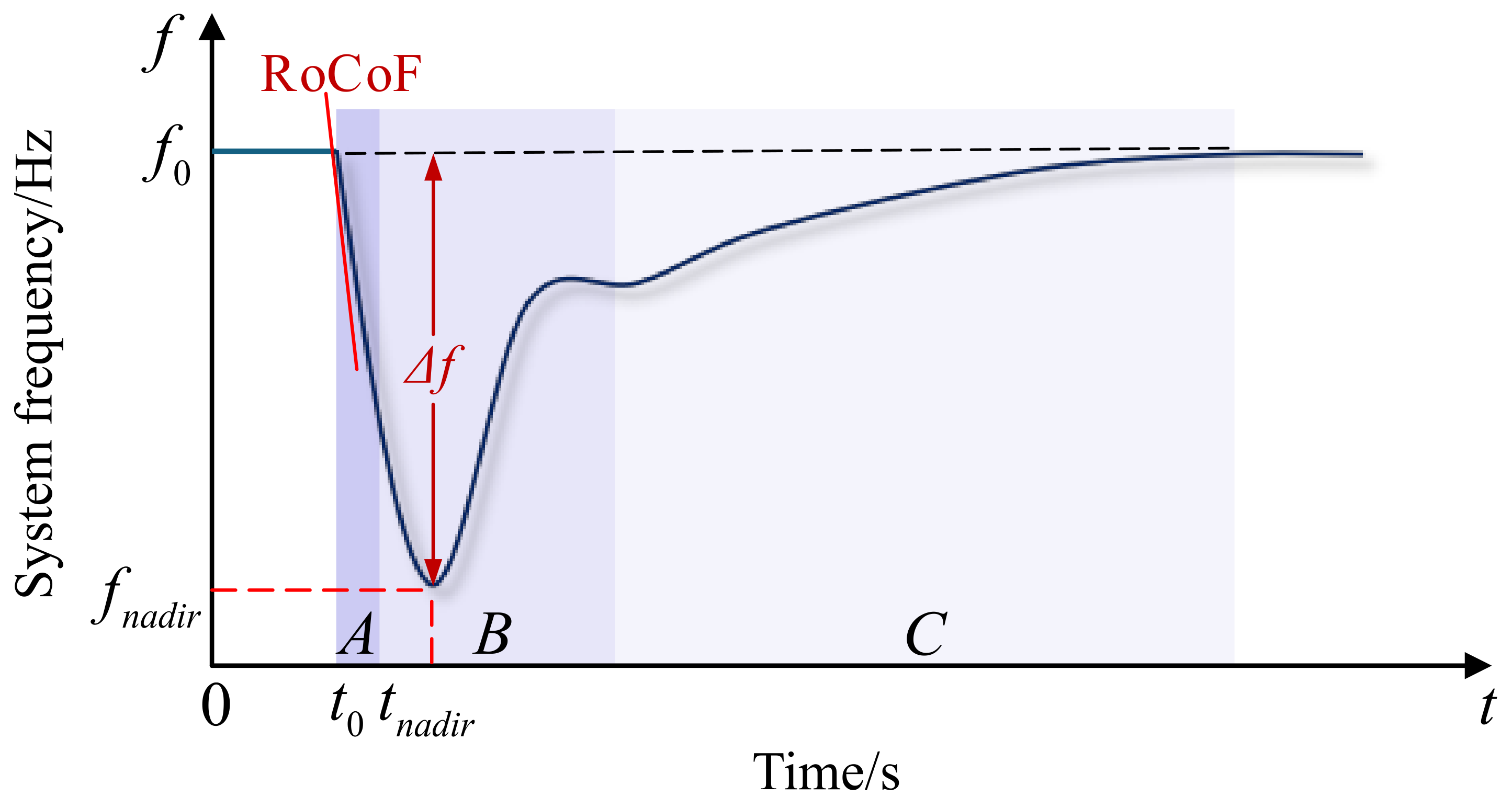
Disturbances, encountered by the power system, are represented by active power deficits. For example, a sudden increase in disturbance power will cause the frequency to drop. Based on the regulation process, the system’s frequency variation can be divided into three main stages, as shown in Figure 2: (A) inertia response stage; (B) co-response stage of inertia and PFR (including fast frequency response from virtual inertia resources); and (C) secondary frequency regulation stage.

2.3. Modeling FSC Incorporating Grid-Forming Resources

It can be seen from the frequency response process that RoCoFmax and the frequency nadir are key characteristics reflecting system frequency security. Inertia plays a role in both phases A and B. A higher level of inertia leads to a smaller RoCoF immediately after a disturbance and effectively supports the system frequency before PFR is activated.
Therefore, this paper selects the following two characteristics as criteria for evaluating the adequacy of inertia levels:
  • R o C o F max : An excessively high R o C o F max may lead to mechanical damage in rotating equipment due to abrupt speed changes, disconnection of distributed generation resources due to protection activation, islanding operation of the system, and oscillations in stabilizers [6]. Furthermore, to ensure sufficient time and margin for subsequent PFR, the inertia, in the form of kinetic energy, must satisfy:
    d Δ f ( t ) d t t = t 0 = Δ P e ( t 0 ) D s y s Δ f ( t 0 ) 2 E s y n f 0 R o C o F max
    where R o C o F max represents the maximum tolerable rate of frequency change.
  • Maximum Frequency Deviation Δ f ( t n a d i r ) : This is the difference between the steady-state frequency and the frequency nadir. It is influenced by the combined effects of the IR and PFR. To prevent the system from triggering under-frequency load shedding or even a system collapse due to an excessive frequency drop [7], the following condition must be satisfied:
    Δ f ( t n a d i r ) Δ f max
    where t n a d i r is the time at which the frequency nadir occurs, and Δ f max is the maximum allowable frequency deviation for the system.
To obtain the Δ f ( t n a d i r ) , Equation (19) is integrated and solved in conjunction with Figure 1, yielding the expression for the frequency deviation at the time of the system frequency nadir as follows:
Δ f ( t n a d i r ) f 0 2 ( E s y n + E v i r ) [ t 0 t 1 R F F R t t 1 t 0 d t + P F F R max ( t n a d i r t 1 ) + t P F R t n a d i r R P F R t t 2 t P F R d t t 0 t n a d i r Δ P e ( t ) d t D s y s t 0 t n a d i r Δ f ( t ) d t ]
where R P F R and R F F R represent the PFR capability of SGs and the FFR capability of VRE, respectively. P P F R max and P F F R max are the maximum power outputs of synchronous generator PFR and VRE’s FFR, respectively.
Considering the multi-stage frequency response process involving multiple types of virtual inertia resources in a power system with high penetration of RES and incorporating the key characteristics of system frequency dynamics extracted above, FSCs are constructed to ensure that the planning results comply with the rational planning principles for virtual inertia resources.
1.
Constraint on the R o C o F max ;
The R o C o F max constraint will ensure that the planning results satisfy the RoCoF security requirement and is represented by Equation (20).
2.
Minimum System Frequency Constraint
By incorporating the frequency regulation functions of various types of grid-forming resources, the system’s dynamic frequency swing Equation (19) can be equivalently expressed as follows:
d Δ f d t = f 0 2 ( H s y n + H v i r ) g G Δ P g P F R + w W Δ P w P F R + b B Δ P b P F R P l o s s
H v i r = w W H w v i r + v V H v v i r + b B H b v i r
P l o s s = P d i s + P r e c w i n d
where H s y n denotes the synchronous inertia energy of the system, and H v i r denotes the virtual inertia energy; Δ P g P F R , Δ P w P F R , and Δ P b P F R represent the PFR power of conventional units, wind farms, and BESS, respectively.
Assuming that the lowest frequency point after a system disturbance is t * , integrating both sides of the above Equation (25) with respect to time gives the expression for the lowest frequency point of the system, considering the frequency regulation capability of multiple types of virtual inertia resources as follows:
Δ f ( t * ) = f 0 2 ( H s y n + H v i r ) P G P F R ( t * T d e l 2 ) 2 2 T 2 + P B P F R ( t * T d e l 1 T 1 2 ) + P W P F R ( t * T d e l 3 T 3 2 ) P l o s s t *
0 Δ f ( t * ) Δ f max
P G P F R = g G P g P F R
P B P F R = b B P b P F R
P W P F R = w W P w P F R
where Δ f ( t * ) denotes the lowest frequency point of the system, and Δ f max denotes the maximum frequency deviation that the system can withstand; T 1 , T 2 , and T 3 are the PFR delivery times for PV-storage systems, conventional units, and wind farms, respectively; T d e l 1 , T d e l 2 , and T d e l 3 are the PFR response times for PV-storage systems, conventional units, and wind farms, respectively; P G P F R , P W P F R , and P B P F R are the total PFR power of conventional units, wind farms, and PV-storage systems, respectively.
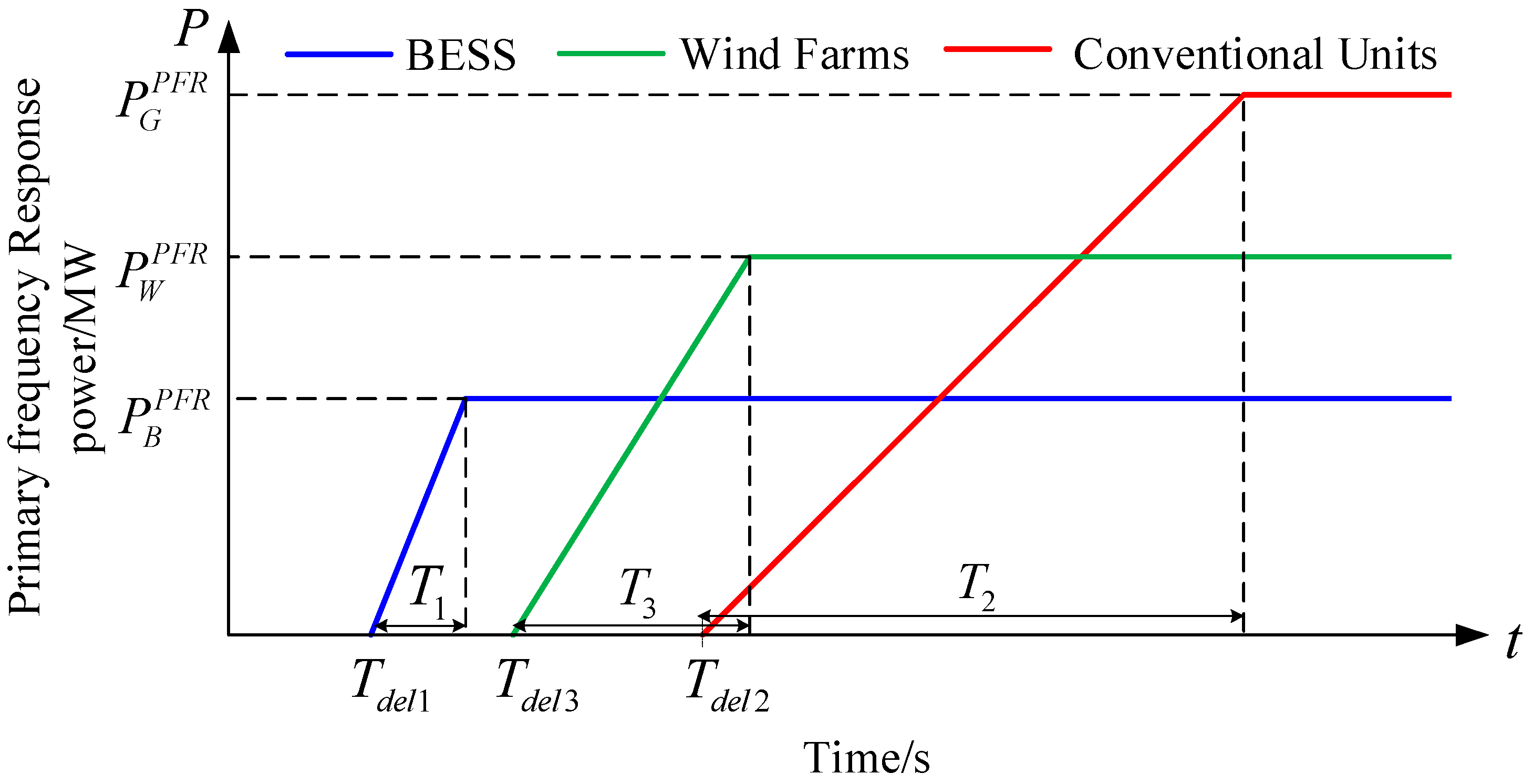
The PFR power response process of the different types of resources is represented by Figure 3. Considering that in the frequency regulation process of the power system with high penetration of RES, the PFR power of conventional units plays the dominant regulatory role, the time corresponding to the system’s lowest frequency point will occur during the PFR process of conventional units. That is, the lowest frequency point occurs within the interval T d e l 2 , T d e l 2 + T 2 . By applying the triangle area formula, the expression for t * can be derived as follows:
t * = ( P l o s s P B P F R P W P F R ) P G P F R T 2 + T d e l 2 .
By substituting Equation (31) into Equation (26), we can derive the inertia level constraint of the security of the system’s frequency nadir as follows:
H s y n + H v i r f 0 2 Δ f max T 2 P W P F R + P B P F R P l o s s 2 2 P G P F R P B P F R ( T d e l 2 T d e l 1 T 1 2 ) P W P F R ( T d e l 2 T d e l 3 T 3 2 ) + P l o s s T d e l 2 .

3. Analysis of the Spatial Distribution Characteristics of Inertia in a Power System with High Penetration of RES

With the continuous increase in the penetration rate of VRE, the heterogeneous virtual inertia it provides will lead to a continuous decline in the inertia level at the nodes where VRE is integrated. This will change the spatial distribution characteristics of inertia levels across the system nodes, resulting in new spatial distribution patterns of frequency response in a power system with high penetration of RES. To identify nodes with weak inertia levels and guide the planning of inertia resources, this section deduces and establishes a nodal frequency response model.
Assume that the power system contains a total of N nodes, including NG generation nodes and NL load nodes. The generation nodes include all power sources that actively participate in the system’s frequency regulation process, such as SGs and VRE units. Neglecting the resistance of the transmission lines, the relationship between nodal power and phase angles can be expressed by Equation (33):
P G P L = B G G B G L B L G B L L δ G δ L
where P G and P G represent the injection power at the generation nodes and load nodes, respectively. B G G and B L L denote the self-susceptance of the generation nodes and load nodes, respectively. B L L and B L G represent the mutual susceptance between the generation and load nodes, respectively. δ G and δ L are the voltage phase angles of the generation nodes and load nodes, respectively. Based on Equation (33), the power expression for the generation nodes and the power expression for the load nodes of the system can be derived as Equations (34) and (35):
P G = B G G δ G + B G L δ L
P L = B L G δ G + B L L δ L .
Referring to the concept of Kron reduction [15,23], and retaining only the frequency dynamics of the generation nodes while equivalently distributing the disturbance power on the load nodes to the individual generation nodes, Equation (35) can be transformed as follows:
δ L = B L L P L B L G δ G 1 .
Substituting the above equations into Equation (34) and rearranging yields the power for the generation nodes as Equation (37), which incorporates the equivalently coupled disturbance power from the load nodes.
P G = B ^ G G δ G + T ^ G L P L
where B ^ G G is the equivalent susceptance matrix between generation nodes, and T ^ G L is the weighting matrix that distributes the disturbance power from the load nodes to each generation node. It is worth noting that Kron simplification is sensitive to input data errors of nodes connected by extremely low impedance branches in the network. In this case, appropriate network pre-equivalent or numerically robust pseudo inverse techniques can be applied before calculation [24]. Substituting Equation (37) into the frequency swing Equation (38) of the generation node matrix, and assuming that the prime mover regulation speed is much slower than the change in electromagnetic power (ΔPm=0), the expression for the RoCoFmax of the generation node matrix can be derived by neglecting damping as Equation (39):
2 H G d Δ ω d t + D G Δ ω = Δ P m Δ P e
d Δ ω G d t = 1 2 H G T ^ G L 1 Δ P L .
To map the inertia distribution of the entire power system to the generator nodes, the frequency response at each node in the system can be regarded as the superposition of the frequency responses from each generator node based on the system’s network topology [25]. Combined with the nodal disturbance power distribution matrix T ^ G L , the expression for the RoCoFmax of the system node matrix can be derived as follows:
d Δ ω J d t = T ^ G L T d Δ ω G d t .
Then, the system nodal computational inertia matrix expression is defined as follows:
H J = Δ P L 2 d Δ ω J d t .
Combining Equation (39) and Equation (40), the computational inertia matrix expression for system node i can be formulated as follows:
H J , i = 1 T ^ L G , i H G , i T ^ G L , i 1 .
Equation (42) represents the nodal computational inertia expression, which depends solely on the system’s network topology and the inertia levels at the generator nodes. This allows for the mapping and evaluation of the computational inertia levels at various nodes within the system based on the inertia levels at the generator nodes, thereby enabling an assessment of the spatial distribution characteristics of the system’s inertia levels.

4. A Bi-Level Robust Planning Model of Grid-Forming BESS and VRE Considering Frequency Security

This section establishes a bi-level robust planning model for grid-forming BESS and VRE, taking frequency security into account. The coordination of VRE is achieved by retrofitting VRE plants to have grid-forming virtual inertia capabilities. To balance the economy and security of the planning results, operational simulation is embedded into the planning model, which ensures power and energy balance under typical scenarios while guaranteeing frequency security during system operation.

4.1. Objective Function

The objective function, which is given by Equation (43), is to minimize the total annual investment cost C Inv and operational cost C Ope . The investment cost includes costs for wind power, PV systems, and BESS, as shown in Equation (44). The system operational cost aims to minimize the daily generation cost, carbon emission cost, and the penalty for VRE curtailment under typical daily scenarios, as expressed in Equation (45):
min C total = C Inv + C Ope
C Inv = w c W C w W + v c V C v V α 1 ( 1 + α 1 ) T l i f e 1 ( 1 + α 1 ) T l i f e 1 1 + b c B C b B + b c E E b B α 2 ( 1 + α 2 ) T l i f e 2 ( 1 + α 2 ) T l i f e 2 1
C Ope = max U min t Ξ , p Ψ 365 r π r t { g ( c g P i , t , r + c e E i , t , r ) + w W , v V c c u r [ ( P w , t , r u + P v , t , r u ) ( P w , t , r + P v , t , r ) ] }
where c W and c V represent the power capacity and energy capacity planning cost for wind power, PVs and BESS, respectively. c B and c E represent the power planning cost and capacity planning cost of the BESS, respectively. C w W and C v V represent the power capacity and energy capacity planning size for wind power and PV systems, respectively. C b B and E b B represent the power capacity planning size and energy capacity planning size of the BESS, respectively. α 1 , T l i f e 1 and α 2 , T l i f e 2 represent the discount rate and service life for wind power/PVs and BESS, respectively. c g and c e represent the power generation cost and carbon emission cost of thermal power units, respectively. c c u r represents the penalty cost for VRE curtailment. P i , t , r and E i , t , r are the power output and carbon emissions of thermal power units on a typical day, respectively. P w , t , r u and P v , t , r u represent the forecasted power output of wind and PV power on a typical day, respectively. P w , t , r and P v , t , r represent the actual VRE output of wind and PV power on a typical day, respectively. r represents the index of the r-th typical day.

4.2. Constraints on the Planning of Multiple Types of Grid-Forming Resources

1.
Operational Model of BESS
The decision variables of the BESS planning model include: the location, rated power, and capacity of the BESS. The decision variables are as follows:
x = ζ n , P n B , E n B
where ζ n is a binary variable indicating whether the n-th BESS unit is deployed, and E n B represents the planned capacity of the n-th BESS unit.
Equation (47) represents the BESS siting constraint, which ensures that BESS is deployed at the proposed location with the shortest electrical distance to the node (the node with the minimum inertia). The calculation method for the nodal inertia is provided in Section 2. Equation (48) limits the maximum number of BESS to be deployed. Equations (49) and (50) define the constraints on the planned power rating and energy capacity of the BESS, respectively:
E ( a ) = G ( a ) : min ( d B ( G ( a ) , a H min ) )
n ζ n N B max
P n B = ζ n P ^ n B
ζ n E _ n B E n B ζ n E ¯ n B
where E(a) is the set of BESS planning nodes. G(a) is the set of generator nodes. a H m i n is the node with the minimum inertia. dB is the electrical distance between two nodes. N B max is the upper limit of the planning quantity. P n B is the allocated power of the BESS. E _ n B and E ¯ n B are the lower and upper limits of the BESS capacity planning, respectively.
2.
Investment Cost and VRE Retrofit Constraints
VRE stations are configured through grid-forming virtual inertia support retrofits. Other planning constraints of the model include: the system investment cost budget constraint Equation (51), and the maximum retrofittable. capacity constraints Equations (52) and (53) for VRE units:
C Inv Π max
0 C w W C max W
0 C v V C max V
where Π max is the upper limit of the planned cost. C max W and C max V are the maximum retrofittable. capacities of the wind farm and PV power station, respectively.

4.3. Typical Day Operational Constraints

1.
Nodal Power Balance Constraints
The nodal power balance constraint ensures instantaneous active power balance at each node within the system:
g G ( m ) P g , t , r + w W ( m ) P w , t , r + v V ( m ) P v , t , r + b B ( m ) ( P b , t , r d i s P b , t , r c h ) l L ( m ) P l , t , r = d D ( m ) P d , t , r m , t , r
where Pg,t,r is the actual output of the thermal power unit, Pl,t,r is the power flow on line l, and Pd,t,r is the load size at node d.
2.
Line Power Flow Constraints
The line power flow constraints include node phase angle stability constraints and line maximum transmission capacity constraints:
P l , t , r = ( θ m , t . r θ o , t , r ) / x l l , t , r
P l max P l , t , r P l max l , t , r
θ m min θ m , t . r θ m max m , t , r
where θm,t,r is the phase angle of the node, x l is the reactance of line l, and P l m a x is the maximum transmission power limit of the line l.
3.
Thermal Power Unit Operational Constraints
The operational constraints for thermal power units include output upper and lower limit constraints Equation (58), startup and shutdown time constraints Equations (59) and (60), ramp rate constraints Equation (61), and annual operating hours constraints Equation (62):
u g , t , r ξ G C g G P g , t , t u g , t , r C g G g , t , r
X g , t 1 , r o n T o n , g u g . t 1 , r u g , t , r 0 g , t , r
X g , t 1 , r o f f T o f f , g u g , t , r u g , t 1 , r 0 g , t , r
R g D R P g , t , r P g , t 1 , r R g U R g , t , r
r t 365 π r u g , t , r h max g , t , r
where X g , t , r o n and X g , t , r o f f are the continuous operating and shutdown time of the unit. T o n , g and T o f f , g are the minimum continuous operating and shutdown time of the unit. R g D R and R g U R are the upward and downward ramp rates of the unit output. h max is the maximum annual operating hours of the unit.
4.
VRE Output Constraints
Considering the short-term uncertainty of VRE such as wind and PV, robust optimization techniques are employed in the planning model to meet the system’s flexible regulation requirements. The uncertainty set is a key concept in robust optimization, ensuring that the selected decisions remain feasible for any realization of uncertainty within such a set. The uncertainty set shown in Equation (63) is adopted to model VRE output [26]. Equations (64) and (65) represent the output constraints for wind and PV power generation under uncertain scenarios:
U = p w , t , r u = p w , t , r f + z w , t , r + Δ p w , t , r + z w , t Δ p w , t , r p v , t , r u = p v , t , r f + z v , t , r + Δ p v , t , r + z v , t Δ p v , t , r z w , t , r + + z w , t , r 1 , z v , t , r + + z v , t , r 1 , w , v , t   z w , t , r + , z w , t , r , z v , t , r + , z v , t , r 0 , 1 t z w , t , r + + z w , t , r Γ T W , t z v , t , r + + z v , t , r Γ T V ,
0 P w , t , r p w , t , r u C w W
0 P v , t , r p v , t , r u C v V
where p w , t , r f , p w , t , r u and p v , t , r f , p v , t , r u are the forecasted output and uncertain output of wind and PV power on a typical day, respectively. z w , t , r + , z w , t , r , z v , t , r + , z v , t , r are the uncertainty control variables. Δ p w , t , r + , Δ p w , t , r and Δ p v , t , r + , Δ p v , t , r are the forecast errors of wind and PV power output, respectively. Γ T W and Γ T V are the temporal uncertainty budgets for wind and PV power output, respectively.
5.
BESS Operational Constraints
Refer to the Equation (2) to Equation (18) in Section 2.1 of this paper.
6.
Frequency Security Constraints
Refer to Equation (20) and Equation (32) in Section 2.3 of this paper.

4.4. Model Solution

4.4.1. Linearization of the FSC

As shown in Section 2.3, Equation (32) represents a complex nonlinear constraint containing quadratic terms. Through mathematical derivation, Equation (32) is transformed into the form of Equation (66) to convert it into a linear second-order cone programming (SOCP) constraint:
H s y n + H v i r f 0 P B P F R ( T 1 + 2 T d e l 1 ) 4 Δ f max P W P F R ( T 3 + 2 T d e l 3 ) 4 Δ f max + P G P F R T d e l 2 2 4 T 2 Δ f max P G P F R T 2 P l o s s P B P F R P W P F R + P G P F R T d e l 2 / T 2 2 Δ f max 2 .
The definitions of the physical quantities in the equation have been clearly defined in Section 2.3. To simplify the computation, based on the second-order cone programming (SOCP) model shown in Equation (66), the product terms in the Equation (66) are substituted using elements A ˜ , B ˜ , and C, which can be expressed as the following:
A B C 2
A ˜ = H s y n + H v i r f 0 P B P F R ( T 1 + 2 T d e l 1 ) 4 Δ f max P W P F R ( T 3 + 2 T d e l 3 ) 4 Δ f max + P G P F R T d e l 2 2 4 T 2 Δ f max
B ˜ = P G P F R T 2
C = P l o s s P B P F R P W P F R + P G P F R T d e l 2 / T 2 2 Δ f max .
Through substitutions, Equation (66) can be transformed into the following:
A ˜ + B ˜ A ˜ B ˜ 2 + 4 C 2 .
Thus, Equation (71) can be transformed into the form of a two-norm:
A ˜ + B ˜ A ˜ B ˜ 2 C
A B C 2 .
Equation (73) is the linearized expression of the frequency nadir constraint. It is worth noting that the unit of the inertia constant in Equation (66) is MW·s. Through structural reorganization, the dimension of variable A ˜ is MW·s/Hz, the dimension of variable B ˜ is MW/s, and the square of variable C has the dimension MW2/Hz, which ensures dimensional consistency in Equation (73).

4.4.2. Model Solution Based on Nested C&CG Algorithm

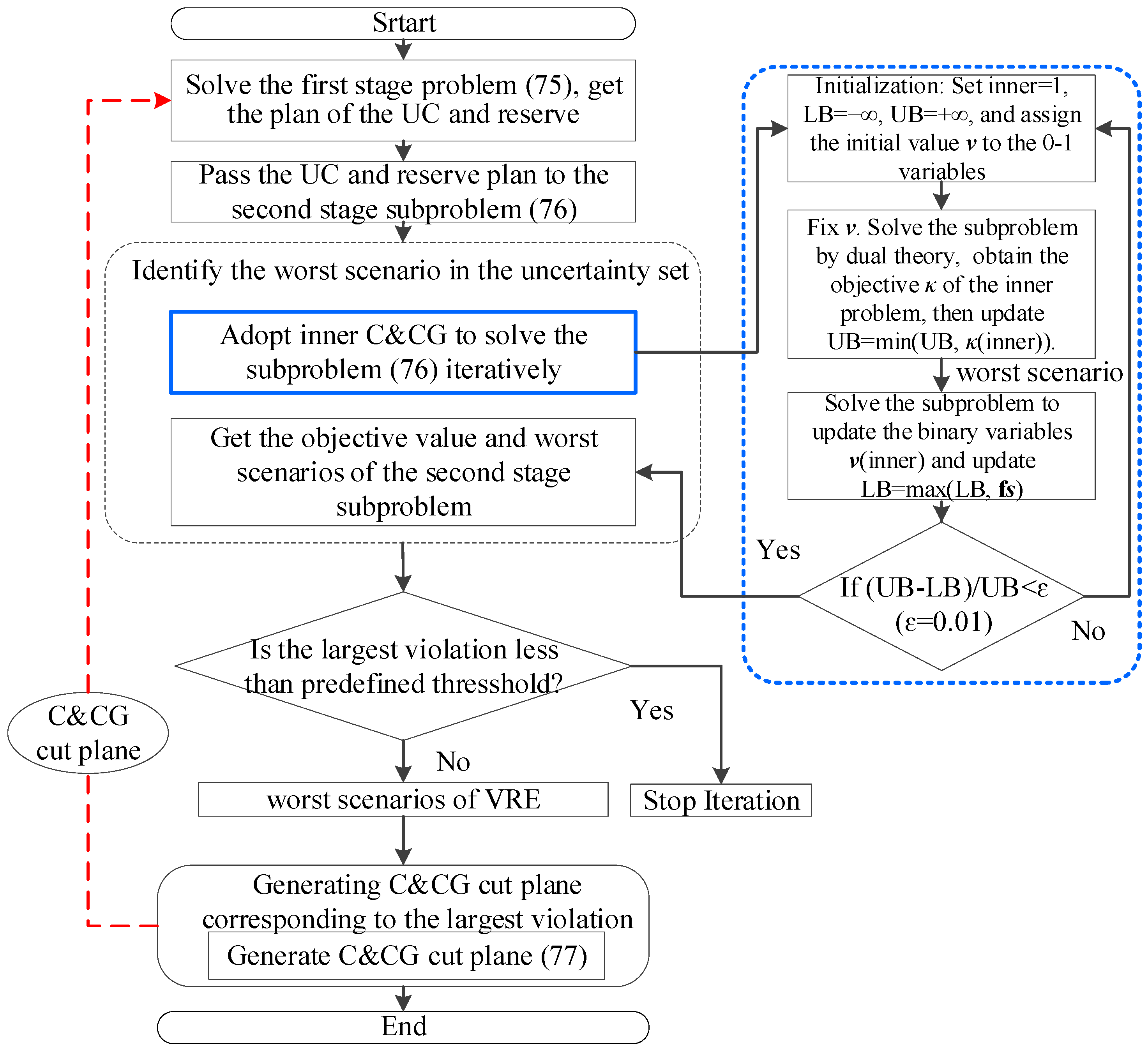
The solution process of the established grid-forming resource planning model is divided into two steps: planning and capacity determination. This section solves the planning model iteratively through upper-level and lower-level subproblems. The upper-level planning model guides the BESS planning and the grid-forming virtual inertia retrofitting of wind farms and PV-storage power plants. The lower-level operational optimization layer determines the capacity of the selected BESS and the retrofitting capacity of wind and PV-storage facilities, with uncertainties characterized by a robust optimization method. The planning result is obtained through iterative cycles between the upper and lower levels. The planning model is solved using the C&CG algorithm, as shown in Figure 4.
First, the model is expressed in the matrix form shown in Equation (74):
min x , c   a T c + max p w u ,   p v u U   min v , p Ξ ( c , p u ) b T p u + e T p w u + f T p v u s . t .   A x + B c g     E x + H c + F p u + G p w u + K p v u + Q v 1       p u 0       x , v 0 , 1
where x and c are the vectors of binary variables and continuous variables under the basic scenario, respectively. v and p u are the vectors of binary unit commitment variables and output of conventional units under VRE output uncertainty scenarios, respectively. p w u and p v u are the vectors of wind farm and PV output, respectively. A, B, E, H, F, G, K, Q, a , b , e , f , and g are constant coefficient matrices and vectors. The specific algorithm solution process is as follows (Algorithm 1):
Algorithm 1: Improved column-and-constraint generation algorithm
1:Enter Outer-Layer C&CG:
2:Initialization: Set the iteration count iter = 0.
3:while iter < itermax do
4:   Solve master problem Equation (75) (iter):
5:    min x , p , c   a T c + η s . t .    A X + B c g η b T p u + e T p w w o r s t + f T p v w o r s t C & CG   Benders   Cut   from   the   subproblem x 0 , 1 (75)
6:   Let ( x i t e r , p i t e r ) be the optimal solution;
7:   Solve Subproblem Equation (76) (iter):
8:    ψ = max p w , u p v u min p u , v u , s b T p u + e T p w w o r s t + f T p v w o r s t s . t .   E x i t e r + H c i t e r + F p u + G p w u + K p v u + Q v u + M s 1   p u 0   v u 0 , 1   p w u ,   p v u U (76)
9:   Obtain ( x o u t e r , p o u t e r );
10:   Invoke Inner-Layer C&CG:
11:   Initialization: Set iinner ← 1, LB ← , UB ← + ;
12:  Initialize binary variable vector v.
13:  while True do
14:   Solve Dual Problem Equation (77) (iter):
15:    max η μ , p w u , p v u κ s . t .     κ ( η μ ) T ( 1 E x i t e r H c i t e r F p u Q v μ G p w u K p v u ) F η μ 0 M η μ 0 η μ 0                 o r           unlimited p w u 0 ,         p v u 0   1 μ i i n n e r (77)
16:   Let (κ, p w w o r s t , p v w o r s t ) be the optimal solution;
17:   Update UB ← min{UB, κ}.
18:   Fix p w u p w w o r s t , p v u p v w o r s t ;
19:   Solve the optimization problem for v in the subproblem to obtain slack s;
20:   Update LB ← max{LB, fs}.
21:    if  UB LB / UB < ε , ε = 0.01 then
22:     ψ ← UB;
23:     return (ψ, p w w o r s t , p v w o r s t );
24:     Return to outer layer.
25:    else
26:     iinneriinner + 1.
27:    end if
28:  end while
29: (ψ, p w w o r s t , p v w o r s t ) ← Inner C&CG ( x i t e r , p i t e r );
30: if ψ > 0 then
31:  Generate cut;
32:  Generate new variables siter +1, pu iter+1, viter+1;
33:  Add a new C&CG Benders cut to the master problem;
34:  Update iteration iteriter + 1.
35: else
36:  Termination x* ← xiter, p* ← piter;
37:  break.
38: end if
39:end while

5. Case Studies

5.1. Modified NPCC-140 Bus System Case Study

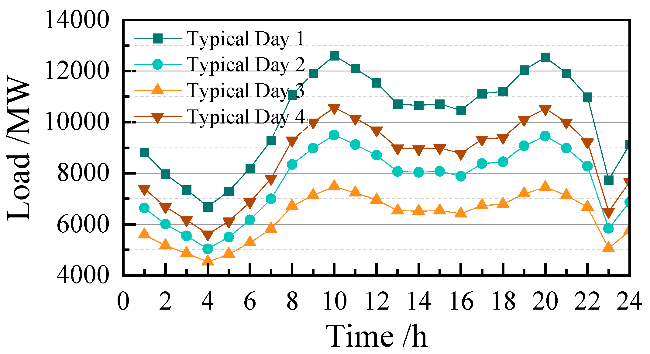
This section uses a modified NPCC-140-bus system [26] for case study analysis to demonstrate the effectiveness of the proposed method. The system includes conventional synchronous generation with an installed capacity of 18.15 GW, wind power capacity of 4 GW, and PV capacity of 16 GW, resulting in a VRE penetration rate of 52.4%. The system peak load is 12.6 GW. Based on historical grid data clustering, four typical daily scenarios for wind power, PV output, and load demand are generated, with VRE output uncertainty set at 10%. Key case study data and the resource portfolio of the modified NPCC-140-bus system are provided in Appendix A. With reference to power system frequency security regulations [27], the R o C o F max limit is set at 0.5 Hz/s, and the frequency nadir limit is set at 59.8 Hz.
Specifically, the computer configuration used is: Intel Core i7-14700KF CPU @ 3.40 GHz, NVIDIA GeForce RTX 4070 Ti SUPER graphics card, and 32 GB RAM. The proposed planning model was implemented using the Yalmip language in Matlab 2020b and solved with the Gurobi optimizer 10.0.1.

5.2. Planning Results and Cost Analysis

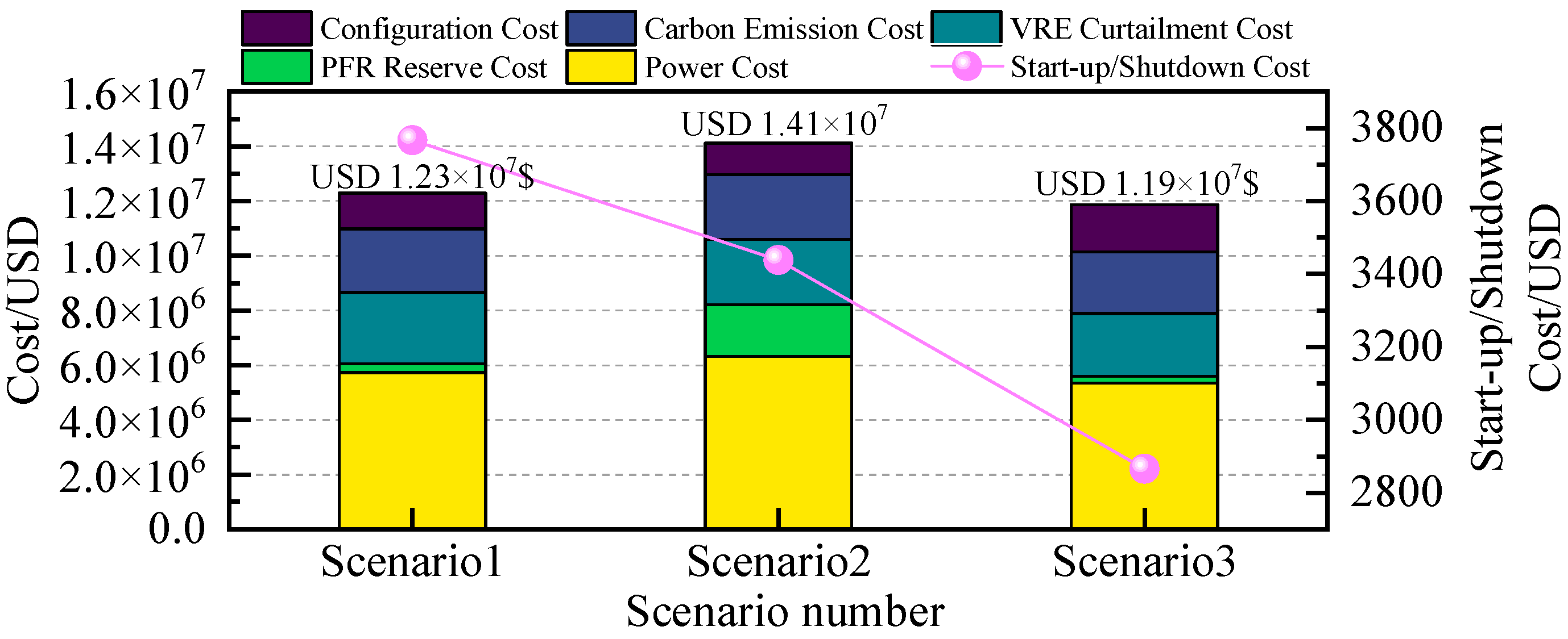
To validate the effectiveness of the proposed method, three comparative scenarios considering system frequency security and VRE uncertainty are designed, as shown in Table 1, to investigate the role of collaborative planning of multiple types of grid-forming resources. Among them, Scenario 1 represents the scheme with only wind and solar virtual inertia retrofits; Scenario 2 is the planning scheme with only BESS; Scenario 3 is the collaborative planning scheme combining BESS with wind and solar virtual inertia retrofits. The results are shown in Table 2 and Figure 5.
Table 2 presents the planning results of multiple types of grid-forming resources under each scenario. As shown in Table 2, Scenario 3 reduces the required power and energy capacity of BESS compared to Scenarios 1 and 2, and also decreases the virtual inertia retrofit capacity for wind farms. This is attributed to the collaborative planning of BESS and wind-solar virtual inertia retrofits, which leverages the complementary advantages of wind power and PV-storage systems in providing virtual inertia support across different time periods. This synergy alleviates the demand pressure for virtual inertia support that would otherwise be imposed by a single type of resource planning.
Figure 5 shows the planning results and total system costs for each scenario. As shown in Figure 5, Scenario 2 (with only BESS planning) exhibits the highest total system cost among the three scenarios. This is because the frequency regulation capability of BESS is weaker than that of VRE units, forcing the system to rely heavily on the PFR power of thermal units to meet frequency security requirements. This leads to higher costs associated with PFR reserve power. In contrast, Scenario 3, through the collaborative planning of multiple resource types, reduces the total system cost by 3.3% and 15.9% compared to Scenarios 1 and 2, respectively. This reduction is achieved by leveraging the flexible charging and discharging advantages of BESS, which enhances the system’s ability to accommodate VRE. Additionally, the three types of resources collectively provide virtual inertia support, reducing the pressure for virtual inertia resource planning and further lowering costs. The planning results of Scenario 3 demonstrate the effectiveness of the proposed method.

5.3. Analysis of the Impact of FSC on Planning Results

5.3.1. The Impact on Planning Results of FSC

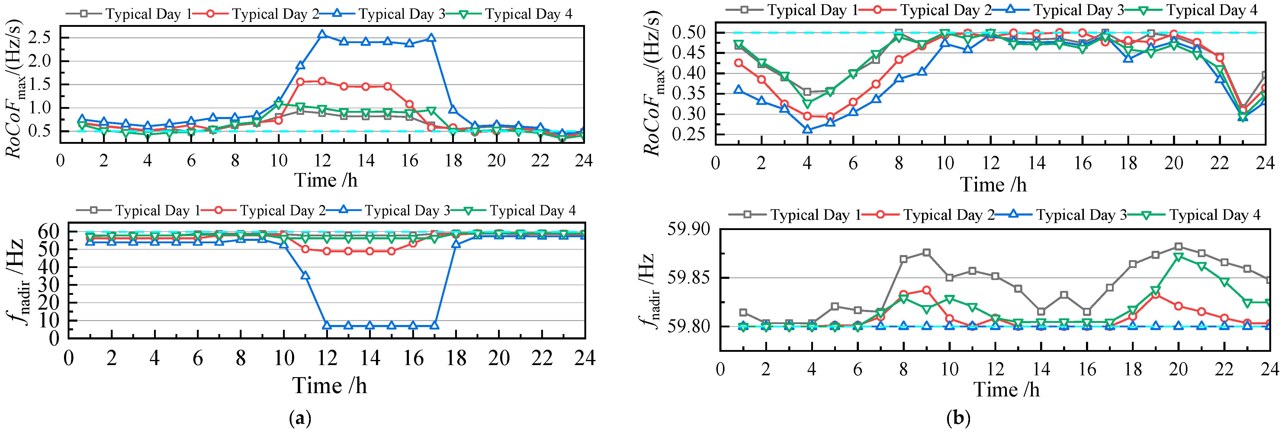
To verify the impact of FSC on planning results, the influence of these constraints on planning outcomes was investigated under conditions that account for the uncertainty of VRE. A comparative analysis was conducted by setting up planning scenarios both with and without FSC. The results are shown in Table 3 and Figure 6.
Table 3 presents the planning results with and without FSC. As shown in Table 3, the scenario considering FSC requires higher BESS power and capacity, as well as greater virtual inertia retrofitting capacity for wind and solar power, compared to the scenario that disregards these constraints. This is because the FSC introduced in the former scenarios increases the system’s demand for virtual inertia resources, thereby further enhancing system frequency security.
Figure 6 illustrates the characteristics of system frequency security indicators with and without FSC, respectively. A comparison of the two figures reveals that in the scenario without FSC shown in Figure 6a, the system’s minimum frequency points exceed the limits during 10~18 h. In contrast, in the scenario with FSC shown in Figure 6b, all minimum frequency points remain within the required limits. This improvement is attributed to the multiple types of virtual inertia resources configured in the frequency-constrained scenarios, which meet the system’s support needs and enhance its inertia support and frequency regulation capabilities. These results demonstrate the effectiveness of FSC.
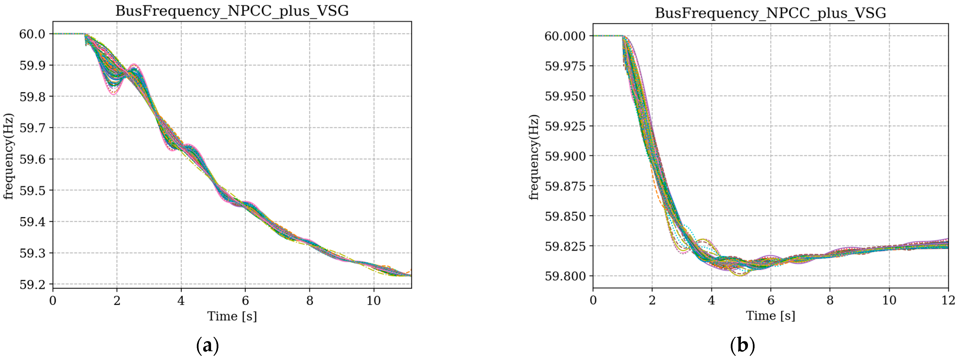
To further verify the actual frequency response, time-domain simulations were performed for both planning outcomes under the same system operating point (corresponding to 2 h of a typical day). A power disturbance of the same magnitude was set at t = 1.0 s. The dynamic responses, simulated using the Andes library in Python 3.10.0 [28], are compared in Figure 7, confirming the enhanced frequency security with FSC.

5.3.2. Sensitivity Analysis of FSC Constraints to Frequency Security Thresholds

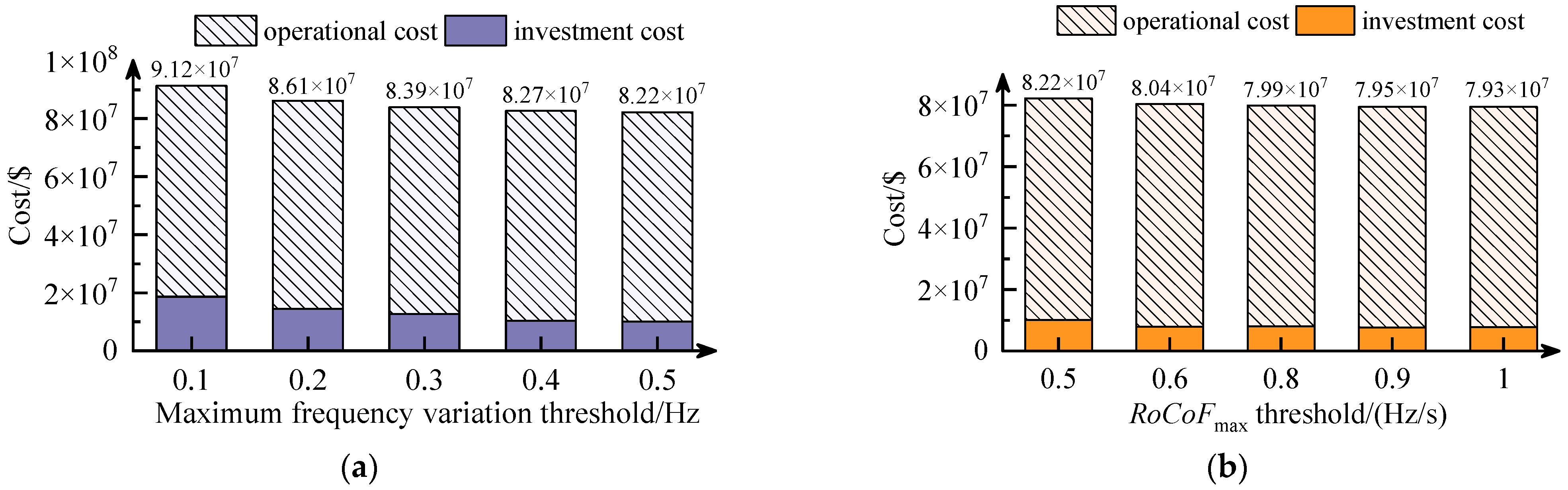
To validate the effectiveness of the proposed FSC and analyze the impact of its key thresholds on system planning results, this section presents a sensitivity analysis. Based on the same test system, the analysis investigates the sensitivity of the total system planning cost to the maximum frequency variation threshold and the RoCoFmax threshold. The various resources planning results obtained are shown in Table 4. The variation in total system cost is shown in Figure 8.
(1) Sensitivity Analysis on the Maximum Frequency Variation Threshold
With the RoCoFmax = 0.5 Hz/s, the maximum frequency variation threshold was gradually relaxed from 0.1 Hz to 0.5 Hz. Figure 8a shows that the total cost shows a decreasing trend as the threshold is relaxed, with a reduction of roughly 9.86%. At the same time, the overall scale of resource allocation in Table 4 also decreases. This is because relaxing this threshold reduces the system’s demand for PFR resources, thereby decreasing the need for flexible regulation resources that must be configured to meet frequency security requirements. This directly lowers both the operational and investment costs of the system. The results indicate that the total system cost is quite sensitive to changes in this threshold.
(2) Sensitivity Analysis on the RoCoFmax Threshold
With the maximum frequency variation threshold fixed at 0.5 Hz, the RoCoFmax threshold was relaxed from 0.5 Hz/s to 1 Hz/s in Figure 8b. In contrast to the maximum frequency variation threshold, the total system cost is much less sensitive to changes in the RoCoFmax threshold, with a reduction of about 3.5%. This is because the RoCoFmax threshold primarily constrains the system’s inertia level at the instant of a disturbance. Its relaxation mainly affects the configuration of SGs or virtual inertia resources, which has a limited impact on the PFR resources required for sustained action. Consequently, its marginal effect on the total cost is smaller.
Through comparison, it is evident that the maximum frequency variation threshold has a greater influence on the total cost than the RoCoFmax threshold. The above analysis demonstrates that the proposed FSC can effectively quantify the economic cost associated with frequency security requirements.

5.3.3. Sensitivity Analysis of the Selection of Delay Times T F F R d and T F F R c

To investigate the impact of the grid-forming BESS frequency regulation parameters, sensitivity analyses are conducted for the T F F R d and T F F R c . The planning results are shown in Table 5.
Firstly, with T F F R c fixed at 5 s, T F F R d varies from 0.1 s to 0.9 s. The results indicate that as T F F R d increases, the required BESS power rating and energy storage capacity exhibit a decreasing trend, dropping from 3600 MW to 1200 MW. Conversely, the required retrofit capacity for renewable energy sources to provide virtual inertia shows a clear increasing trend, rising from a combined 2654 MW to 5423 MW. Notably, the BESS configuration saturates at 1200 MW for T F F R d values between 0.7 s and 0.9 s.
Secondly, with T F F R d fixed at 0.5 s, T F F R c is varied from 2 s to 12 s. The required BESS power and storage capacity increased significantly, from 1800 MW to 4800 MW. In contrast, the total virtual inertia retrofit capacity for VRE resources demonstrates a general decreasing trend, falling from approximately 3590 MW to 4000 MW. Similar to the first case, the BESS configuration reaches saturation at 4800 MW for T F F R c values between 10 s and 12 s.
These trends can be explained by the role of grid-forming BESS as a flexible virtual inertia provider. A BESS with low T F F R d and low T F F R c can provide swift virtual inertia support, effectively mitigate the fnadir and reduce the system’s reliance on other resources, thereby lowering the total planning cost. An excessively long T F F R c severely undermines the BESS’s ability to provide immediate virtual inertia support during the initial transient. To compensate for this deficiency, the system is forced to allocate a larger BESS capacity to meet the FFR requirement, explaining the sharp increase in BESS rating with longer T F F R c . Conversely, an overly long T F F R d prevents the BESS from contributing effectively during the critical first moment of post-disturbance. This incapacity shifts the burden of inertia support, prompting the system to expand and rely more heavily on virtual inertia retrofits for wind and PV power plants.

5.4. Impact of Grid-Forming Resource Planning on the Inertia Spatial Distribution

5.4.1. Inertia Spatial Distribution Results

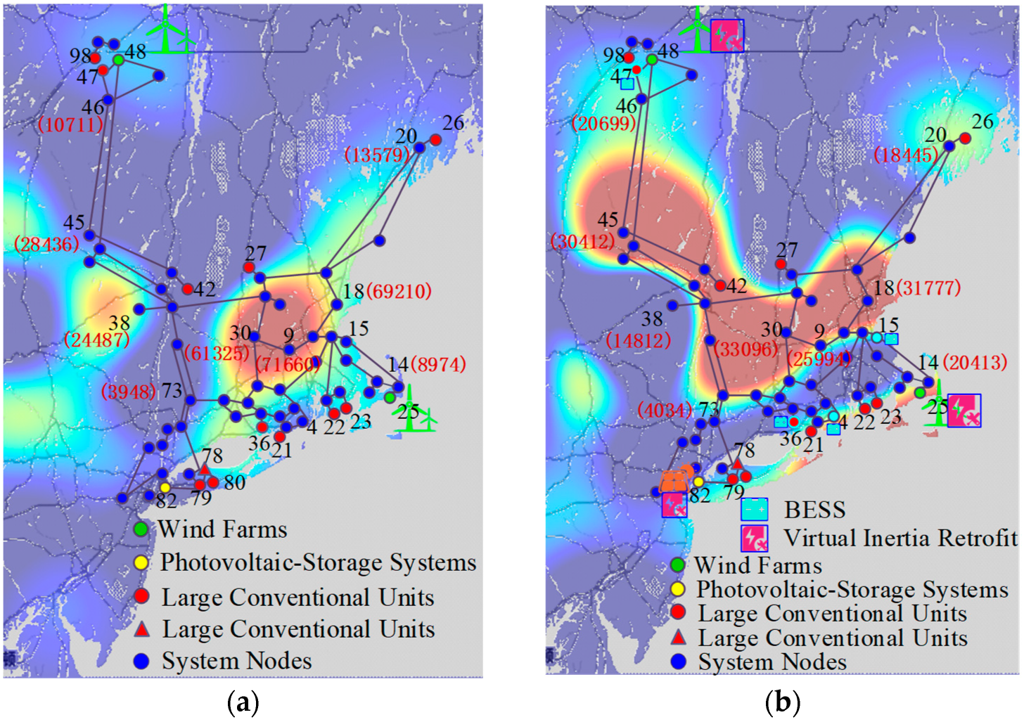
To analyze the impact of grid-forming resource planning on the spatial distribution of system inertia, a comparative analysis of the spatial distribution of system inertia was conducted by controlling the planning decision variables before and after the planning of grid-forming resources. Based on the calculation model for the spatial distribution of system inertia mentioned in Section 2 of this paper, the augmented matrix of system power nodes after the planning of BESS was calculated. The results of the partial spatial distribution of inertia before and after the planning of virtual inertia resources are shown in Figure 9, with some nodes marked in red numbers indicating their inertia levels, in units of MWs.
Figure 9 demonstrates that configuring BESS and virtual inertia resources (Figure 9b) creates a more uniform spatial inertia distribution compared to the base scenario (Figure 9a). The background thermal map, where redder areas indicate higher local inertia, shows a transition from a few intense red spots to a more widespread, moderate red coverage, indicating improved balance.
Specifically, previously weak nodes like 46, 45, and 14 show dramatically increased inertia values (e.g., node 46 rising from 10,711 to 20,699 MWs). Conversely, previously excessive nodes like 38, 30, 9, and 18 show significant reductions (e.g., node 9 dropping from 71,660 to 25,994 MWs). This improvement is achieved by retrofitting wind farms, PV-plus-storage systems with grid-forming virtual inertia support and deploying additional BESS. The planning of multiple types of virtual inertia resources optimizes the overall inertia distribution across all nodes, strengthens inertia at weak points, and leads to a more balanced spatial distribution of system inertia.

5.4.2. Sensitivity Analysis to Line Reactance Uncertainty

To verify the robustness of the proposed Kron reduction-based spatial inertia distribution method against line parameter uncertainty, a sensitivity analysis is conducted on line reactance under the same network configuration and parameters as shown in Figure 9b. Nodes 20 and 45 are selected as representative cases. The reactance values of the key lines connecting them to their respective source nodes (Line 20–26 and Line 45–46) varied by ±5% and ±10% of their nominal values. The resulting inertia calculations are summarized in Table 6.
As shown in Table 6, the standard deviations of the calculated inertia for both nodes remain relatively low within the given range of reactance variation, indicating that the proposed method exhibits good robustness against parameter uncertainty. A further comparison reveals that the standard deviation for Node 20 is noticeably smaller than that for Node 45. This difference can be primarily attributed to their respective electrical distances to the source nodes. Node 20 is electrically closer to source Node 26, making its inertia calculation less sensitive to variations in the connecting line parameter, whereas Node 45 is located farther from source Node 46, thus showing greater parameter sensitivity. Nevertheless, the ratios of the standard deviation to the mean inertia are only 0.16% and 0.27% for the two nodes, respectively, both of which are acceptably low.
This suggests that typical uncertainties in line reactance have a limited overall impact on the spatial inertia distribution results, remaining within an acceptable range for engineering applications.

5.5. Analysis of the Impact of VRE Uncertainty on Planning Results

5.5.1. The Impact on Planning Results of VRE Uncertainty

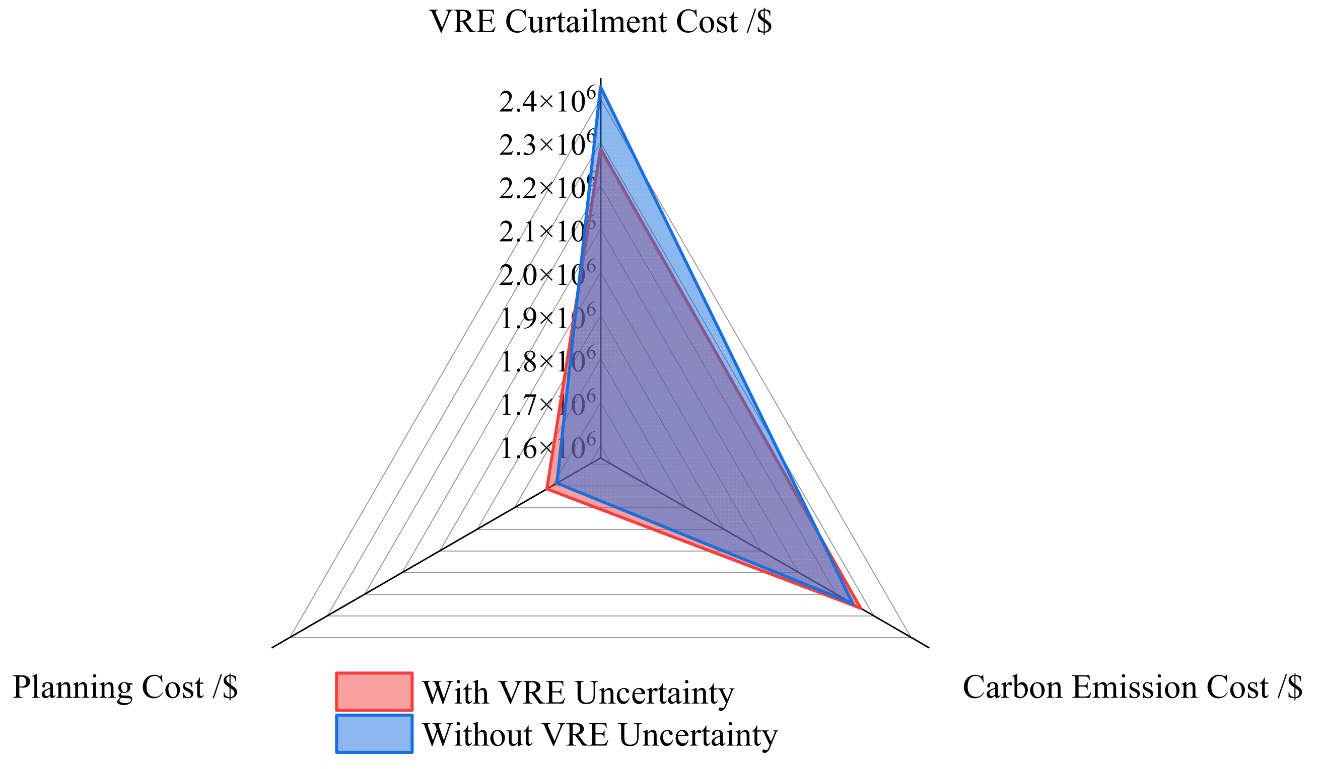
To analyze the impact of VRE generation uncertainty on planning results, a comparative study was conducted by examining planning outcomes with and without consideration of 10% VRE uncertainty, under the condition that FSC are taken into account. Planning scenarios were established both with and without the uncertainty constraints for comparative analysis. The results are presented in Table 7 and Figure 10.
Table 7 presents the planning results with and without consideration of VRE uncertainty constraints. As shown in Table 4, the scenario considering uncertainty requires a higher resource planning capacity compared to the scenario that does not. Specifically, to maintain system security under uncertainty, the required BESS power/energy capacity doubles (a 100% increase from 1200 MW to 2400 MW), and the required wind power retrofit capacity increases by approximately 228% (from 624 MW to 2050 MW). The PV retrofit capacity also sees a substantial increase from 128 MW to 1000 MW.
Furthermore, partial cost results for different scenarios in Figure 10 indicate that the scenario considering uncertainty incurs higher resource planning costs and carbon emission costs, but lower VRE curtailment costs than the scenario without such consideration.
This is because the uncertainty-aware scenario configures a greater capacity of BESS and VRE virtual inertia retrofitting under the constraints. Leveraging the flexible charging and discharging advantages of BESS enhances the system’s VRE accommodation capacity, thereby reducing curtailment costs. Additionally, it appropriately increases the power output of thermal power units to buffer fluctuations in VRE, further optimizing the power balance of system operation.

5.5.2. Sensitivity Analysis of the Temporal Uncertainty Budgets Γ T W and Γ T V for VRE

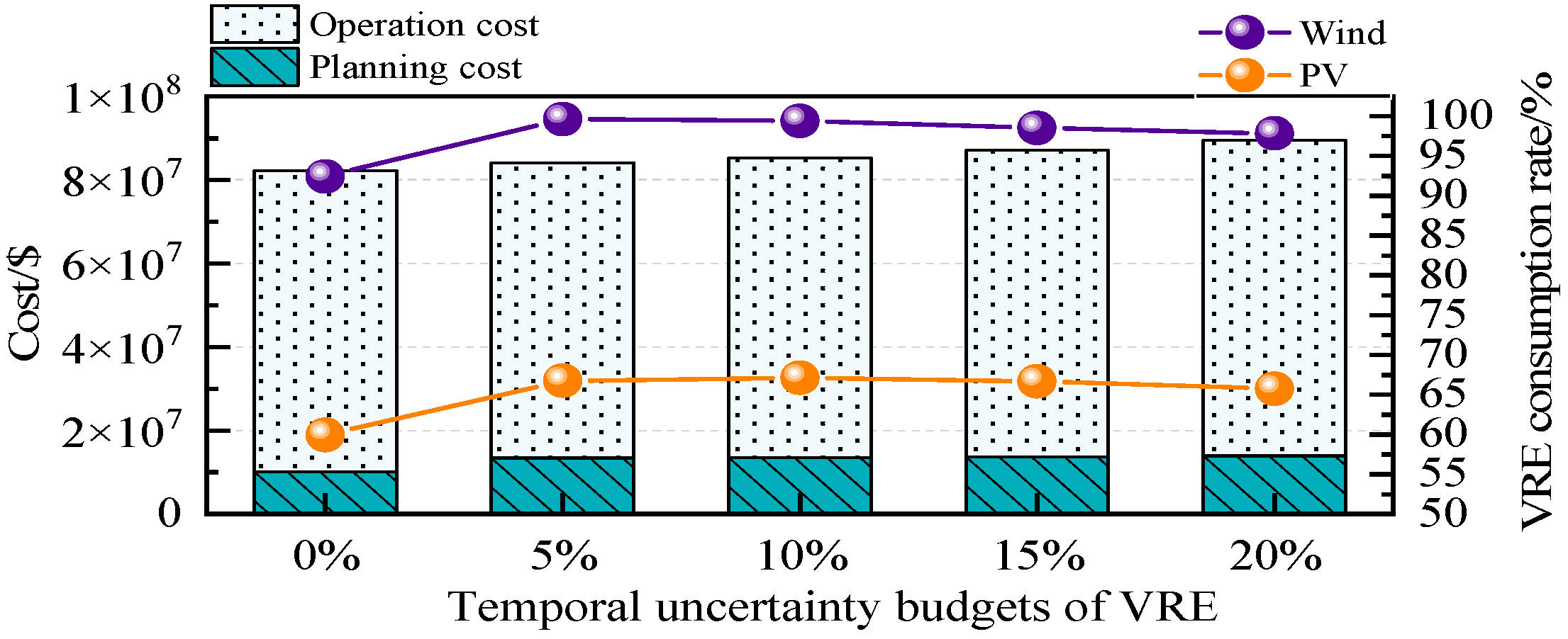
To thoroughly demonstrate the consideration of the uncertainty budget for VRE output in this paper, this section presents a sensitivity analysis. The impact of varying the uncertainty budget Γ T W and Γ T V (for the sake of analysis, it is assumed that the two are the same) from 0% to 20% on planning results, total system cost, and VRE consumption rate is compared and analyzed as shown in Table 8 and Figure 11.
In Figure 11, when the uncertainty budgets are 0%, the VRE consumption rate is relatively low, while the total system cost remains comparatively lower. At the same time, the overall scale of resource allocation in Table 8 also increases. This is because the model does not account for the uncertainty of renewable energy output, leading to insufficient configuration of frequency regulation resources, which weakens the system’s ability to accommodate VRE. After considering the uncertainty of VRE output, the VRE consumption rate increases significantly. As the uncertainty budgets grow, the total system cost gradually rises, while the VRE consumption rate remains at a satisfactory level without being disturbed by the volatility of VRE output. This indicates that the robust optimization method proposed in this paper for addressing VRE output uncertainty is effective and exhibits good sensitivity.

5.6. Effectiveness of the Solution Algorithm

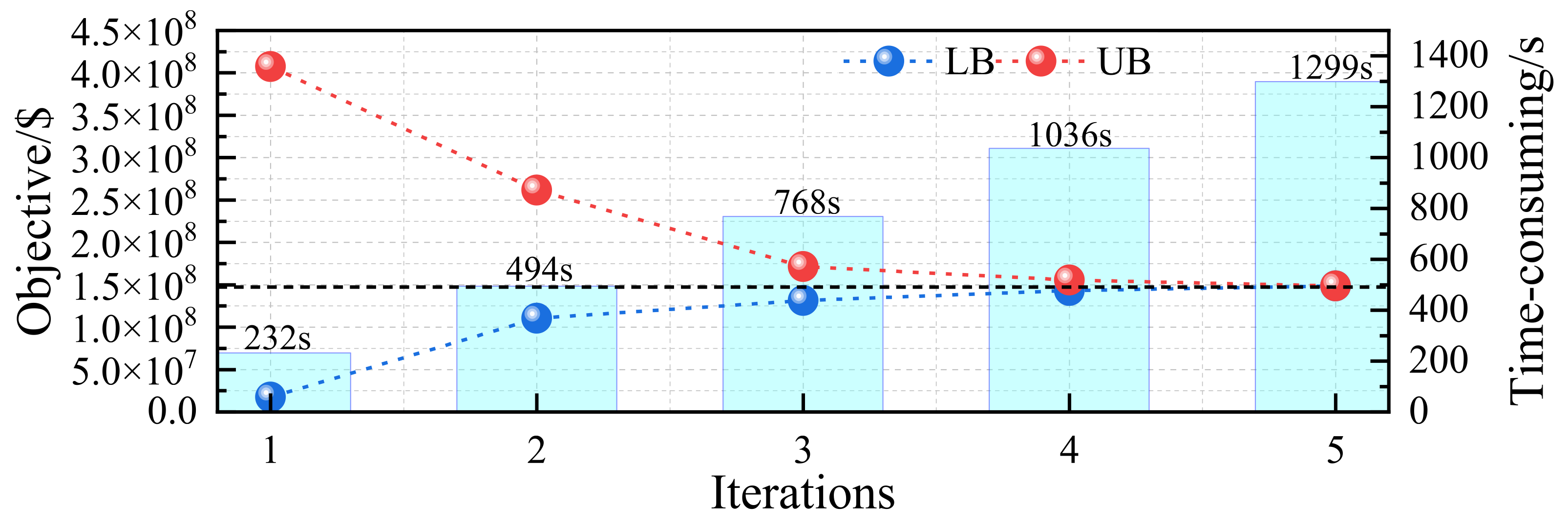
This paper proposes an improved C&CG algorithm to solve the robust planning problem, considering the uncertainty of renewable energy output in the model. The computational convergence process and cumulative iteration time for Scenario 3 are shown in Figure 12.
As the number of iterations increases, the upper and lower bounds of the objective gradually converge. After five iterations, with a convergence gap of 0.1%, the operating cost converges to USD 1.19 × 10⁷, at which point the cumulative time is 1299 s. It can be seen that the improved C&CG algorithm effectively solves the robust planning model, and its relatively high computational efficiency demonstrates potential for practical engineering applications.
Overall, the proposed wind–storage frequency regulation framework offers a practical and technically sound solution to the frequency stability challenges associated with high renewable energy penetration and extreme weather events. The findings underscore the critical role of coordinated control strategies in enhancing system reliability and pave the way for broader deployment of hybrid renewable–storage planning in future low-carbon power systems.

6. Conclusions

To ensure frequency security in a power system with high penetration of RES with a high penetration of VRE, this paper proposes a bi-level robust planning model for grid-forming energy storage considering renewable energy uncertainty and FSC. The following conclusions are drawn from the case study analysis:
(1)
The system frequency dynamics modeling, which accounts for the response delay of VSG, can accurately characterize the VIR of grid-forming resources. Guiding BESS planning based on the spatial distribution calculation method of system inertia effectively mitigates the uneven distribution of inertia caused by VRE integration. This method enhanced the system’s frequency security support capability, ensuring RoCoF of each node remained below 0.5 Hz/s and the frequency nadir above 59.8 Hz under the considered disturbance in the planning study.
(2)
The proposed cooperative planning model for multiple types of grid-forming resources effectively balances the economy and security of the planning results. By linearizing nonlinear FSC via second-order cone convex optimization, the planning scheme not only satisfies the frequency security threshold but also reduces the total cost by up to 15.9% compared to a single-resource solution. Specifically, the optimal cooperative plan involved deploying 2400 MW/4800 MWh of BESS alongside retrofitting 2050 MW of wind power and 1000 MW of PV capacity with grid-forming capabilities, demonstrating cost-effective resource synergy.
(3)
The proposed cooperative optimization planning method can effectively mitigate the impact of VRE uncertainty. By adopting a nested C&CG robust optimization algorithm, the model leverages the flexible charging and discharging advantages of BESS. This ensures the reliability of planning results under uncertainty, reducing the VRE curtailment rate and improving VRE accommodation, while necessitating a robust plan that increased BESS capacity by 100% and wind retrofit capacity by approximately 228% compared to a deterministic scenario.
The frequency security analysis and resource planning method proposed in this paper provide an effective technical approach for the secure and stable operation of power systems with high penetration of RES, offering theoretical guidance and reference for the construction and resource planning of future power systems.

Author Contributions

Conceptualization, Y.Y. and X.J.; methodology, Z.F. and Y.Y.; software, X.J.; validation, C.C.; formal analysis, Y.W.; investigation, Y.Y.; resources, Y.Y.; data curation, X.J.; writing-original draft preparation, Z.F. and C.C.; writing—review and editing, Y.W. All authors have read and agreed to the published version of the manuscript.

Funding

This research was funded by the Science and Technology Project of China Electric Power Research Institute Co., Ltd. “Research on Grid Forming Energy Storage Planning Method Considering Source Grid Coordination in Weak Support Power Grid” (52550024000P).

Data Availability Statement

The original contributions presented in this study are included in the article. Further inquiries can be directed to the corresponding author.

Conflicts of Interest

Authors Yijia Yuan, Zheng Fan, Xirui Jiang, Yanan Wu and Chengbin Chi were employed by the company China Electric Power Research Institute. The remaining authors declare that the research was conducted in the absence of any commercial or financial relationships that could be construed as a potential conflict of interest.

Abbreviations

The following abbreviations are used in this manuscript:
BESSBattery energy storage system
VREVariable renewable energy generation
VSGVirtual synchronous generator
RESRenewable energy sources
C&CGColumn-and-constraint generation
SGsSynchronous generators
RoCoFRate of change of frequency
PVPhotovoltaic
FSCFrequency security constraints
PFRPrimary frequency regulation
IRInertia response
VIRVirtual inertia response
SOCState of charge

Appendix A

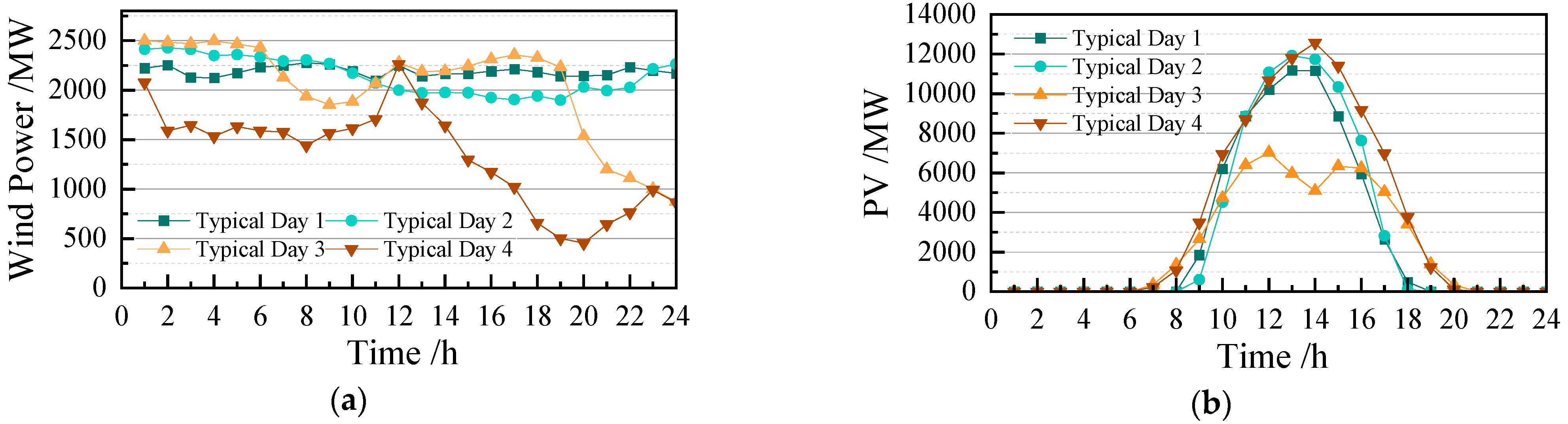
  • The wind power, PV, and load data for the typical day scenarios used in the case studies of this paper are shown in Figure A1 and Figure A2. The capacity of major generation resources in the modified NPCC-140 bus test system is provided in Table A1.
Figure A1. Forecasted VRE curve for a typical day: (a) wind power and (b) PV.
Processes 14 00090 g0a1
Figure A2. Load forecast curve for a typical day.
Processes 14 00090 g0a2
Table A1. Capacity of generation resources in the modified NPCC-140 node system.
Resource TypeCapacity/MWResource TypeCapacity/MW
Thermal Power1165Nuclear Power300
Conventional Hydropower250Wind Power400
Pumped Storage Hydropower100PV1600
2.
Considering the range of cost variations, the costs for grid-forming BESS planning and the grid-forming virtual inertia retrofitting of wind and PV power in the case studies of this paper were comprehensively determined, along with the relevant system operational parameters, as shown in Table A2. The BESS planning capacity must ensure a continuous discharge duration of 2 h.
Table A2. Parameters of VRE generation resources in the modified NPCC-140 node system.
ParametersValuesParametersValues
BESS Rated Power/MW600Wind Farm Lifespan/years20
BESS Capacity Planning Range/MWh[0,1200]PV Power Station Lifespan/years30
BESS Unit Capacity Cost/(USD/MWh)200,000BESS Lifespan/years20
BESS Unit Power Cost/(USD/MW)214,285Carbon Emission Cost/(USD/t)28.57
Wind Power Retrofit Cost/(USD/MW)28,571VRE Curtailment Penalty/(USD/MW)100
PV Retrofit Cost/(USD/MW)357,142BESS Charge/Discharge Efficiency/%0.95
Virtual Inertia Constant/s8Discount Rate/%0.08
3.
In the improved NPCC-140 node system, the grid nodes for VRE integration to be retrofitted and the candidate nodes for BESS planning are shown in Table A3.
Table A3. Candidate nodes of different types of resources in the improved NPCC-140 node system.
Resource TypeWind FarmPVBESS
Candidate nodes25, 4856, 822, 4, 5, 9, 15, 36, 47, 57

References

  1. China Electricity Council. 2024–2025 National Electricity Supply and Demand Analysis and Forecast Report. Available online: https://www.cec.org.cn/detail/index.html?3-341403 (accessed on 20 November 2025).
  2. Li, Y.; Gao, S.; Chen, X.; Fan, D.; Zhang, M. Load Frequency Control of Power Systems Based on Deep Reinforcement Learning with Leader–Follower Consensus Control for State of Charge. Processes 2025, 13, 3669. [Google Scholar] [CrossRef] [Scilit]
  3. Pantaleon, E.; Paucara, J.; Saly, R.D. Power Analysis Produced by Virtual Inertia in Single-Phase Grid-Forming Converters Under Frequency Events Intended for Bidirectional Battery Chargers. Energies 2025, 18, 5560. [Google Scholar] [CrossRef] [Scilit]
  4. Nandini, K.K.; Anubhav, K.P.; Sumana, S.R. Machine learning based annual solar energy forecasting for enhanced grid integration of photovoltaic systems. Bull. Electr. Eng. Inform. 2025, 14, 4267–4278. [Google Scholar] [CrossRef] [Scilit]
  5. Nandini, K.K.; Anubhav, K.P.; Shilpi, B.; Sujit, G.M. Smart inverters based technological advancements in future smart grids for improved flexible renewable energy penetration. Discov. Energy 2025, 5, 28. [Google Scholar] [CrossRef] [Scilit]
  6. Qaisar, M.W.; Fang, J. Grid-Forming Converters for Renewable Generation: A Comprehensive Review. Energies 2025, 18, 4565. [Google Scholar] [CrossRef] [Scilit]
  7. Zhang, Z.; Zhou, M.; Wu, Z.; Liu, J.; Liu, S. Energy Storage Location and Capacity Planning Method Considering Dynamic Frequency Support. Proc. CSEE 2023, 43, 2708–2721. [Google Scholar] [CrossRef]
  8. Zhang, Y.; Yu, Y.; Zhang, Y.; Chen, B.; Liu, Z. Frequency Regulation Performance of a Wind–Energy Storage Hybrid System During Turbine Shutdown Due to Extreme Wind. Processes 2025, 13, 3383. [Google Scholar] [CrossRef] [Scilit]
  9. Silva, A.; Amaro, M.; Mirez, J. Design of a Fuzzy Logic Control System for a Battery Energy Storage System in a Photovoltaic Power Plant to Enhance Frequency Stability. Energies 2025, 18, 4550. [Google Scholar] [CrossRef] [Scilit]
  10. Zhong, Q.; George, W. Synchronverters: Inverters that Mimic Synchronous Generators. IEEE Trans. Ind. Electron. 2011, 58, 1259–1267. [Google Scholar] [CrossRef] [Scilit]
  11. Li, H.; Zhang, X.; Wang, Y.; Zhu, X. Virtual Inertia Control of DFIG-based Wind Turbines Based on the Optimal Power Tracking. Proc. CSEE 2012, 32, 32–39. [Google Scholar] [CrossRef]
  12. Yang, Y.; Wu, Z.; Quan, X.; Xiong, J.; Wan, Z.; Wei, Z. A Unified Control Strategy Integrating VSG and LVRT for Current-Source PMSGs. Processes 2025, 13, 3432. [Google Scholar] [CrossRef] [Scilit]
  13. Simon, D.R.; Pieter, T.; Barry, R.; Dirk, V.H.; Johan, D. Trading energy yield for frequency regulation: Optimal control of kinetic energy in wind farms. IEEE Trans. Power Syst. 2021, 30, 2469–2478. [Google Scholar] [CrossRef] [Scilit]
  14. Assogna, R.; Ciabattoni, L.; Comodi, G. PSO-Based Supervisory Adaptive Controller for BESS-VSG Frequency Regulation Under High PV Penetration. Energies 2025, 18, 5401. [Google Scholar] [CrossRef] [Scilit]
  15. Liu, R.; Wang, Z.; Wu, J.; Zhao, T.; Chan, Y. Planning Optimization of Virtual Inertia Considering Spatial Distribution Characteristics of Frequency. Autom. Electr. Power Syst. 2024, 48, 122–130. [Google Scholar]
  16. Huang, D.; Sun, P.; Yao, W.; Liu, C.; Zhai, H.; Gao, Y. Bi-Level Planning of Grid-Forming Energy Storage–Hydrogen Storage System Considering Inertia Response and Frequency Parameter Optimization. Energies 2025, 18, 3915. [Google Scholar] [CrossRef] [Scilit]
  17. Zhu, L.; Dong, K.; Tang, L.; Li, Z.; Yu, J. Joint Optimal Clearing Model for Electric Energy, Inertia and Primary Frequency Response Considering Synchronous Inertia and Energy Storage Virtual Inertia Values. Proc. CSEE 2024, 44, 7543–7555. [Google Scholar] [CrossRef]
  18. Zhu, Y.; Qin, L.; Yan, Q.; Wei, Z. Wind-storage combined frequency regulation strategy and optimal planning method of energy storage system considering process of frequency response. Electr. Power Autom. Equip. 2021, 41, 28–35. [Google Scholar] [CrossRef]
  19. Ding, Q.; Zhang, X.; Zhang, N.; Li, Z.; Li, W. A Joint planning and Planning Method for Power System Inertia and Primary Frequency Regulation Reserve Considering Extreme Events. Proc. CSEE 2024, 1–17. Available online: http://kns.cnki.net/kcms/detail/11.2107.TM.20240829.1246.008.html (accessed on 18 October 2025).
  20. Zhou, M.; Wang, W.; Li, X.; Li, P.; Chen, Y. A Coordinated Control Strategy for Black Start of Wind Diesel Storage Microgrid Considering SOC Balance of Energy Storage. Processes 2025, 13, 3770. [Google Scholar] [CrossRef] [Scilit]
  21. Cui, H.; Konstantinopoulos, S.; Osipov, D.; Wang, J.; Li, F.; Tomsovic, K.L. Disturbance Propagation in Power Grids with High Converter Penetration. Proc. IEEE 2023, 111, 873–890. [Google Scholar] [CrossRef] [Scilit]
  22. Li, Y.; Hu, P.; Cao, Y.; Yu, Y. Data-driven Estimation Method for Inertia Parameters of Grid-forming Converter Considering Frequency Response Delay. Autom. Electr. Power Syst. 2024, 48, 80–88. [Google Scholar]
  23. Dörfler, F.; Bullo, F. Kron reduction of graphs with applications to electrical networks. IEEE Trans. Circuits Syst. 2013, 60, 150–163. [Google Scholar] [CrossRef] [Scilit]
  24. Yang, N.; Zeng, S. Three-phase power flow solution for multi-grounded four-wire residential networks considering neutral grounding. Energy Build. 2024, 323, 114784. [Google Scholar] [CrossRef] [Scilit]
  25. Zhang, Z.; Guo, Z.; Zhou, M.; Wu, Z.; Bo, Y.; Chen, Y.; Li, G. Equalizing multi-temporal scale adequacy for low carbon power systems by co-planning short-term and seasonal energy storage. J. Energy Storage 2024, 84, 111518. [Google Scholar] [CrossRef] [Scilit]
  26. Joe, H.C.; Graham, R. User Manual for Power System Toolbox, Version 3.0. 2008. Available online: https://sites.ecse.rpi.edu/~chowj/ (accessed on 20 November 2025).
  27. GB/T 15945-2008; General Administration of Quality Supervision, Inspection and Quarantine of the People’s Republic of China, Standardization Administration of the People’s Republic of China. Power Quality-Frequency Deviation for Power System. Standards Press of China: Beijing, China, 2008.
  28. Cui, H.; Li, F.; Tomsovic, K. Hybrid Symbolic-Numeric Framework for Power System Modeling and Analysis. IEEE Trans. Power Syst. 2021, 36, 1373–1384. [Google Scholar] [CrossRef] [Scilit]
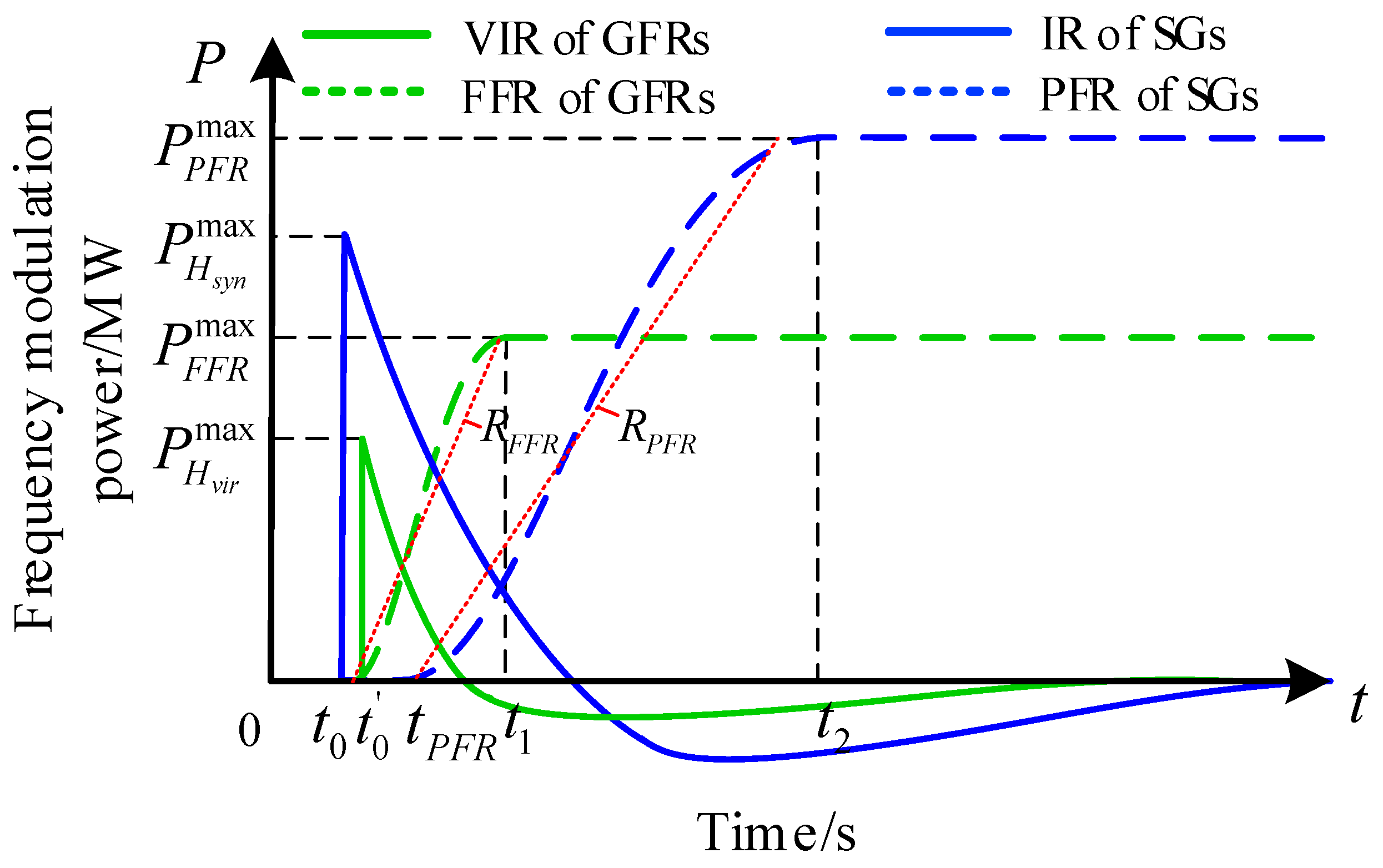
Figure 1. Schematic diagram of power system frequency regulation and power response.
Processes 14 00090 g001
Figure 2. Schematic diagram of the power system frequency variation.
Processes 14 00090 g002
Figure 3. Diagram of the PFR response process for multiple resource types.
Processes 14 00090 g003
Figure 4. Flowchart of the nested C&CG algorithm.
Processes 14 00090 g004
Figure 5. Composition of total system costs in each scenario.
Processes 14 00090 g005
Figure 6. System frequency security indicators for each time period under different scenarios: (a) without and (b) with FSC.
Processes 14 00090 g006
Figure 7. The second-level transient simulation curve of system frequency for the second hour of a typical day in Figure 6b: (a) without and (b) with FSC.
Processes 14 00090 g007
Figure 8. Sensitivity analysis of FSC under different frequency security thresholds: (a) maximum frequency variation threshold and (b) the RoCoFmax threshold.
Processes 14 00090 g008
Figure 9. Partial inertial spatial distribution of the system in different scenarios: (a) without and (b) with grid-forming resources configured.
Processes 14 00090 g009
Figure 10. The VRE curtailment rate for each scenario.
Processes 14 00090 g010
Figure 11. Sensitivity analysis of temporal uncertainty budgets of VRE.
Processes 14 00090 g011
Figure 12. The objective value and cumulative time consumption for each iteration.
Processes 14 00090 g012
Table 1. Scenario settings.
ScenarioMultiple Types of Grid-Forming
Resources
FSCVRE
Uncertainty
BESSWind PowerPV
Scenario 1×
Scenario 2××
Scenario 3
Table 2. Planning results of multiple types of grid-forming resources in each scenario.
ScenarioMultiple Types of Grid-Forming Resources
BESS Power/MWBESS Storage Power/MWhWind Power Retrofit
Capacity/MW
PV Retrofit
Capacity/MW
Scenario 1××3976950
Scenario 236007200××
Scenario 32400480020501000
Table 3. Planning results of multiple types of grid-forming resources in each scenario.
ScenarioMultiple Types of Grid-Forming Resources
BESS Power/MWBESS Storage Power/MWhWind Power Retrofit
Capacity/MW
PV Retrofit
Capacity/MW
Without FSC12002400624128
With FSC2400480020501000
Table 4. Resource planning results under different maximum frequency variation thresholds.
Maximum Frequency Variation Threshold/Hz
(RoCoFmax = 0.5 Hz/s)
Multiple Types of Grid-Forming Resources
BESS Power/MWBESS Storage Power/MWhWind Power Retrofit
Capacity/MW
PV Retrofit Capacity/MW
0.14800960040001292
0.21800360040001349
0.3240048004000962
0.4240048003372549
0.5180036004000709
RoCoFmax threshold/(Hz/s)
(Maximum frequency variation threshold = 0.5 Hz/s)
Multiple Types of Grid-Forming Resources
BESS Power/MWBESS Storage Power/MWhWind Power Retrofit
Capacity/MW
PV Retrofit Capacity/MW
0.5180036004000709
0.624004800446535
0.818003600402593
0.918003600295650
1.018003600247584
Table 5. Resource planning results under different delay times T F F R d and T F F R c .
T F F R d /s
( T F F R c = 5 s)
Multiple Types of Grid-Forming Resources
BESS Power/MWBESS Storage Power/MWhWind Power Retrofit Capacity/MWPV Retrofit Capacity/MWTotal Cost/USD
0.136007200265407.98 × 107
0.32400480030562318.13 × 107
0.51800360040007098.22 × 107
0.71200240040009658.61 × 107
0.912002400400014239.12 × 107
T F F R c /s
( T F F R d = 0.5 s)
Multiple Types of Grid-Forming Resources
BESS Power/MWBESS Storage Power/MWhWind Power Retrofit Capacity/MWPV Retrofit Capacity/MWTotal Cost/USD
21800360030645267.88 × 107
51800360040007098.22 × 107
83000600040005679.97 × 107
1048009600367601.001 × 108
1248009600400001.006 × 108
Table 6. Node calculation inertia under different line reactance uncertainty.
Node Calculation Inertia/MWsLine Reactance Uncertainty (Line 20–26; Line 45–46)Standard Deviation σ
−10%−5%0+5%+10%
No. 2021,329.821,311.321,286.121,261.721,236.433.48
No. 4522,776.422,741.722,699.122,657.522,622.861.93
Table 7. Planning results of multiple types of grid-forming resources in each scenario.
ScenarioMultiple Types of Grid-Forming Resources
BESS Power/MWBESS Storage Power/MWhWind Power Retrofit
Capacity/MW
PV Retrofit
Capacity/MW
Without VRE Uncertainty12002400624128
With 10% VRE Uncertainty2400480020501000
Table 8. Resource planning results under different temporal uncertainty budgets of VRE.
Temporal Uncertainty Budgets of VREMultiple Types of Grid-Forming Resources
BESS Power/MWBESS Storage Power/MWhWind Power Retrofit Capacity/MWPV Retrofit Capacity/MW
0120024001063561
5%180036002561713
10%180036004000709
15%240048002388984
20%3000600040001002
Disclaimer/Publisher’s Note: The statements, opinions and data contained in all publications are solely those of the individual author(s) and contributor(s) and not of MDPI and/or the editor(s). MDPI and/or the editor(s) disclaim responsibility for any injury to people or property resulting from any ideas, methods, instructions or products referred to in the content.