Abstract
A virtual power plant (VPP) faces multiple uncertainties and temporal coupled decisions when participating as an independent entity in electricity and green markets. A multi-level electricity–green coupled market framework is constructed for a VPP participating as an independent market entity. To address uncertainties in renewable energy outputs and market prices, a risk management method based on conditional value at risk entropy weight method information gap decision theory (CVaR-EIGDT) is proposed. To address the temporal coupled challenges in VPP participation across multi-level electricity–green coupled markets, a multi-stage rolling decision-making method coordinating annual, monthly, and daily scales is proposed, achieving deep coupling in the decision-making sequence of multi-level electricity–green coupled markets. Results show that the proposed model enables adaptive decision-making under varying risk preferences, with decisions exhibiting strong practical adaptability while balancing real-time adjustments and long-term planning. The multi-level electricity–green coupled market framework enhances VPP profitability and resilience, while the CVaR-EIGDT method effectively improves decision-making efficiency across multi-level electricity–green coupled markets.
1. Introduction
Facing global conventional energy crises and pressing environmental challenges, countries worldwide have successively rolled out a suite of emission reduction targets and regulatory policies. Carbon markets and renewable portfolio standards are mechanisms widely adopted by countries to control carbon emissions through a combination of market-based incentives and policy-driven mandates. The power industry is one of the major sources of carbon emissions, hence there exists a deep coupling relationship among the electricity market, carbon market, and renewable portfolio standards.
China, which is currently a multi-electricity market system with medium- and long-term transactions as the mainstay and spot transactions as an important supplement, has been basically established and further improved [1]. The national carbon emission trading (CET) market and the renewable energy green electricity certificate trading (GCT) market are both officially operational [2,3]. Meanwhile, the construction of the electricity futures market has entered an active exploration phase [4].
China’s electricity market, CET market, and GCT market developed relatively late and have, to some extent, drawn on the designs of the electricity, carbon markets, and renewable portfolio standards in European Union (EU) and the United States (U.S.). China’s market mechanisms inherently possess compatibility [5]. The medium- and long-term contract and the future structures of the futures market are aligned with the financial contract systems of mature markets such as PJM in the U.S. and the European electricity market. The CET market is compatible with the EU’s EU Emissions Trading System (EU-ETS) and the U.S.’s Regional Greenhouse Gas Initiative (RGGI), while the GCT market is analogous to the EU’s Guarantees of Origins (GO) market, the U.S.’s Renewable Energy Certificates (RECs) market, and Australia’s Large-scale Generation Certificates (LGCs) market. This compatibility not only reflects the advantages of latecomer status but also provides a solid institutional foundation and broad space for convergence for the China’s market in the process of deepening market-oriented reforms and energy-transition processes.
Against this backdrop of profound global market transformation, various new market entities have emerged and are playing increasingly crucial roles. As a typical representative, the VPP shows higher market arbitrage opportunities compared to traditional entities when participating in diverse markets including the electricity market, electricity futures market, CET market, and GCT market, leveraging its inherent resource diversity.
Ref. [6] establishes a market framework for thermal power to participate in the electricity futures market, the medium- and long-term electricity market, and the spot electricity market. Ref. [7] constructs a market framework for VPPs participating in internal and external electricity retail markets, the CET market, and the GCT market. Ref. [8] establishes a trading framework for VPPs participating in medium- and long-term contracts for the difference (CFD) and the GCT market. Ref. [9] constructs a market framework for VPPs participating in the electricity market, the CET market, and the China-certified emission reduction (CCER) market. Ref. [10] proposes a multi-level market framework for VPPs participating in the “medium- and long-term and spot” electricity market and the “primary and secondary” CET market, where internal resources of VPPs can sign medium- and long-term contracts with VPPs.
However, the existing literature has not systematically integrated the electricity futures market, the medium- and long-term electricity market, the electricity spot market, and CET and GCT markets into a unified framework, nor has it recognized virtual power plants (VPPs) as independent entities eligible to participate in the medium- and long-term, or in the futures market.
While VPPs’ participation in multiple markets enhances their value potential, it also exposes them to a series of complex and intertwined potential risks.
First, diverse markets constitute a complex interconnected system with distinct operational rules. Each market operates independently based on unique mechanisms—such as clearing protocols and settlement cycles—that differ significantly. Moreover, the inherent coupling among these markets presents considerable challenges for VPPs.
Second, distinct price formation mechanisms exist across different markets. More importantly, the complex coupling between markets leads to high price volatility and low predictability.
For uncertainty risk management, two primary approaches are stochastic optimization (SO) and information gap decision theory (IGDT). The former replaces uncertainties with scenarios, which is suitable for situations where the probability distribution information of uncertainty is known [11]. The latter defines the range of uncertainties via predicted value deviation envelopes, requiring no probability distribution [12]. The two approaches can be combined to handle various types of uncertainties [13,14,15,16]. Furthermore, conditional value at risk (CVaR) is integrated into SO to quantify scenario-related risks, forming the CVaR-IGDT risk-management method.
Ref. [17] develops robust optimization strategies and opportunity optimization strategies for integrated energy systems participating in the electricity market based on IGDT. Ref. [18] manages the uncertainties of electricity prices and distributed energy outputs based on SO and IGDT, respectively. Ref. [19] combines CVaR and IGDT to address the uncertainties in concentrating solar power output and electricity spot prices faced by concentrating solar power plants (CSPs). Ref. [20] addresses the uncertainties in system outputs and electricity prices faced by integrated biomass-concentrated solar systems participating in the electricity market, based on CVaR-IGDT.
Despite attempts in the existing literature to combine CVaR and IGDT for uncertainty management, most studies fail to effectively distinguish the weights of distinct uncertainties or incorporate objective weighting methods.
In summary, to address the research gaps identified in the existing literature, under a multi-level coupled market framework, this paper proposes a general trading strategy decision-making method based on CVaR-entropy weight-IGDT (CVaR-EIGDT) and multi-stage rolling. The key contributions and novelty of this paper are as follows:
(1) A multi-level coupled market framework is established, where VPPs participate as independent market entities, consisting of a “futures + medium- and long-term + spot” multi-level electricity market and a “primary CET + secondary CET + GCT” multi-level green market. Using China’s current market development status and future direction as a demonstrative case study, the proposed market framework should also be compatible with international market environments.
(2) A CVaR-EIGDT risk management method to address uncertainties associated with renewable energy outputs and market prices is proposed, with the entropy weight method employed to differentiate the weights of distinct uncertainties objectively.
(3) An annual-monthly-daily coordinated multi-stage rolling decision-making method to realize temporal optimization coordination and deep sequential coupling in multi-level coupled market decisions is proposed.
Table 1 and Table 2, respectively, present a comparison between the market frameworks of this paper and the existing literature, as well as a comparison between the uncertainty management methodology of this paper and the existing literature.

Table 1.
Comparison between the market frameworks of the existing literature and this paper.
Table 2.
Comparison between the uncertainty management methodology of the existing literature and this paper.
2. The Multi-Level Coupled Market Framework Involving VPP Participation
VPPs participate in the multi-level coupled market framework, including the electricity futures market, medium- and long-term market, electricity spot market, CET market, and GCT market, as independent entities, forming a multi-level electricity–green coupled market framework consisting of a “futures + medium- and long-term + spot” multi-level electricity market and a “primary CET + secondary CET + GCT” multi-level green market, as shown in Figure 1.
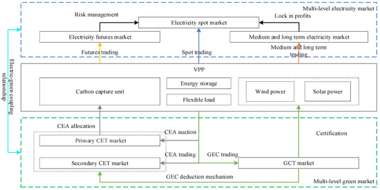
Figure 1.
VPP structure and participation in multi-level electricity–green coupled markets.
The CET market is divided into primary and secondary segments. The primary CET market operates annually prior to the compliance cycle, involving free allocation and paid auction of carbon emission allowances (CEAs) for the upcoming year. Specifically, free CEAs are allocated to carbon capture units within the VPP based on the industry benchmark method, accounting for 70% of the product of the units’ total electricity generation in the previous year and the industry benchmark carbon emission intensity. Additionally, the VPP participates in paid CEA auctions considering factors such as the compliance pressure of its carbon capture units and annual electricity generation plans. The total initial CEAs acquired by the VPP equals the sum of free allocated and paid auctioned allowances.
In the secondary CET market, VPP trades CEAs based on their holdings and year-end compliance obligations. Market participants with carbon emission intensities below the benchmark receive free CEAs exceeding their compliance requirements, which can be sold on the secondary market to gain additional profits. Conversely, those with intensities above the benchmark obtain free CEAs insufficient to meet their obligations, thus needing to purchase additional allowances on the secondary market at extra cost to fulfill compliance. All participants have to fulfill their CEAs compliance obligation at the end of the year; therefore, prior to the compliance cycle conclusion, each can flexibly adjust their CEA holdings based on market prices, buying or selling to minimize transaction costs or maximize profits.
In the GCT market, one green electricity certificate (GEC) is certified for every 1 MWh of renewable energy generated by a VPP. The VPP is required to fulfill its annual GECs compliance obligation by submitting a certain number of GECs based on the renewable energy consumption weighting [21]. Similar to the fulfillment of CEAs compliance obligation, market participants can flexibly trade GECs before the end of compliance cycle. The GCT market must undertake the task of connecting with CEAs offsetting to facilitate the circulation of GECs. This paper assumes that the surplus GECs after fulfilling compliance obligation can offset a certain proportion of the shortfall in CEAs compliance obligation. Notably, the grid-connected electricity of a VPP does not fully equal its total electricity generation, so the GECs certified for the renewable energy electricity in the VPP are divided into tradable GECs and non-tradable GECs based on the grid-connected and self-consumption portions [22]. GECs are certified to the VPP on a daily basis according to its renewable energy generation, with the proportion of tradable GECs equivalent to the ratio of the VPP’s daily grid-connected electricity to its total daily generation (non-tradable GECs account for the remainder). Non-tradable GECs are assumed to be restricted to fulfilling GEC compliance obligations and offsetting CEAs obligations. Both the secondary CET market and the GCT market conduct daily trading subsequent to the settlement of the electricity spot market.
In the electricity futures market, the VPP signs monthly futures contracts for the upcoming year prior to the end of the current year, based on their forecasts of electricity spot prices and potential energy deviations in the spot market. This study assumes that VPPs are only permitted to submit short futures contracts, with all submitted contracts guaranteed to be matched and executed. Each monthly futures contract is automatically decomposed into daily contracts for the corresponding month, with delivery settled at the daily spot market price subsequent to spot market settlement [23].
In the medium- and long-term electricity market, VPP can sign annual and monthly medium- and long-term contracts. Before the year, VPPs sign annual generation contracts as independent entities, which are decomposed by VPPs into monthly plans according to their generation schedules. Before the start of each month, the VPP signs the next monthly contract, which can be flexibly decomposed into each time period of the current month.
In the electricity spot market, a VPP actual grid-connected electricity energy may deviate from the contracted energy in medium- and long-term agreements, driven by factors such as fluctuations in renewable energy output and internal resource dispatching adjustments. VPPs are required to declare their full electricity trading energy for each time moment in the spot market, with any energy deviation from the medium- and long-term contracted energy, settled at the spot price.
As mentioned above, in the proposed multi-level coupled market, VPPs need to conduct trading activities according to the trading sequence and process of each market, as shown in Figure 2.
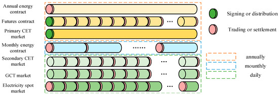
Figure 2.
Time scale relationship diagram of multi-level coupled markets.
At the start of each year, VPPs sign annual energy contracts and electricity futures contracts, with free CEAs allocation in the primary CET market also conducted during this period. Futures contracts are evenly decomposed into daily contracts for settlement. Monthly energy contracts are signed at the beginning of each month. the spot market operates 24-h trading daily, while the secondary CET market and GCT market trade after the spot market closes.
2.1. Coupling Relationship of Spot, Futures, Medium-, and Long-Term Market
The coupling of the spot, medium- and long-term, and futures markets represents a cross-time scale coupling relationship between electricity quantity and price.
The spot market provides real-time price signals and instantaneous transaction mechanisms, dynamically reflecting the real-time supply-dem and balance of the electricity system. Medium- and long-term contracts lock in the energy price for future periods, securing the basic electricity energy profit and separating the medium- and long-term profit risk of VPP from the fluctuations in spot market prices.
The futures market provides efficient and flexible financial instruments to lock in the spot deviation energy price for future periods, adjust the profit from spot deviation energy settlement, and transfer the short-term profit risks of VPP from the fluctuations of spot market prices to the financial market.
2.2. Coupling Relationship of Electricity, CET, and GCT Markets
The output of carbon capture unit, renewable energy outputs, and traded electricity energy within the VPP are dynamically interconnected through carbon emission liability and renewable energy consumption obligations. Specifically, the CET market increases the cost of carbon capture unit, while the GCT market can create additional profits to renewable energy units.
VPPs regulate the carbon emissions and the number of GECs by adjusting the output of carbon capture unit and renewable energy power, respectively. VPP obtains CEAs through CET market transactions to fulfill the carbon compliance obligation arising from the output of carbon capture unit and earns profits by selling excess tradable GECs in the GCT market under the premise of fulfilling the renewable energy consumption compliance obligation. Furthermore, GECs can offset a certain amount of CEA deficits via a dedicated deduction mechanism. Together, these interactions form an integrated “electricity–CET-GCT” coupling relationship.
2.3. Market Assumptions
2.3.1. Price Taker Assumption
Under the trend of improving the construction of provincial electricity spot markets in China and the goal of building a unified national electricity market, market activity is increasing. Meanwhile, the ability of individual market entities to influence electricity prices remains constrained, as the market’s increasingly mature operation and expanded participation base enhance its competitiveness and reduce the pricing power of single participants. For the CET market and GCT market, China has established national trading platforms, and prices are determined by the supply and demand and the situation in the national market. Therefore, this paper considers the participation of VPPs in the market as price takers. Given the booming supply and demand and in China’s electricity market, it is assumed that all bidding strategies made by the VPP in the market can be cleared or executed. This assumption enables the research to focus on the core issues of VPP multi-level coupled market risk decision-making, rather than on the specific details of market microstructure or clearing mechanisms. The price-taker assumption is reasonable when analyzing the VPP’s economic potential and strategic market value [24].
2.3.2. VPP Assumption
To simplify the model and VPP complexity, focus on core issues and improve computational efficiency, concentrating on market strategy optimization rather than physical details. The internal aggregated resources studied in this paper include generalized modeling of carbon capture unit, wind power, solar power, energy storage, and flexible loads; it is assumed that all aggregated resources of the VPP are connected to the same node.
This combination encompasses key functions including dispatchable generation, stochastic generation, regulation-capable resources, and dem and response, which reflect the typical characteristics of a VPP. By adjusting the quantity and proportion of internal resources, this model can flexibly simulate different types of VPP, such as generation-type, load-type VPPs, or VPPs-expanded resource scales. To highlight the core contributions of market trading and uncertainty management methods, this paper focuses on generation-type VPP as the primary research subject, while also providing comparative case analyses of other types of VPPs.
Given the above assumptions, the expected profit calculated in this paper represents a theoretical upper bound. The model proposed is more suitable for evaluating the strategic value and economic potential of VPP.
3. VPP Deterministic Trading Model in a Multi-Level Coupled Market
Based on the VPP multi-level coupled market participation framework constructed in Section 1, a deterministic trading model is established, where uncertainties are replaced with their predicted values.
3.1. Objective Function
The objective function consists of three parts: annual transaction costs of VPP, monthly transaction costs, and daily transaction and dispatching costs. The annual transaction costs include annual electricity energy contracts, monthly futures contracts, and primary CET market transaction costs; the monthly transaction costs include monthly electricity energy contract transaction costs; the daily transaction costs include spot electricity energy transaction costs, secondary CET market transaction costs, GCT market transaction costs, futures contract settlement costs, power generation costs, and flexible load electricity profits and dispatching costs.
represent the total transaction cost of VPP’s annual, monthly, and daily transaction costs, respectively; and represent the annual electricity contract price and contracted electricity volume of VPP, respectively; and represent the auction price of the primary CET market and auction volume of VPP, respectively; and represent the monthly peak load and off-peak electricity futures contract costs, respectively; and represent the monthly electricity contract price and contracted electricity energy of VPP per month; , , and represent the spot market prices at each moment and the positive and negative deviation electricity energy of VPP in the spot market, respectively; represents the dispatching cost of VPP, represents the power generation cost of carbon capture unit. and represent the daily price of the secondary CET market and the volume of CEAs purchased and sold by VPP in the secondary CET market per day, respectively; and represent the daily GECs price and the volume of GECs purchased and sold by VPP in the GCT market per day, respectively; and represent the peak load and off-peak futures delivery costs, respectively.
3.2. Constraints
3.2.1. Annual Constraints
Annual constraints include transaction constraints for markets at the beginning of the year and compliance constraints at year-end.
- Constraints of annual electricity energy contract
and represent the electricity quantity decomposed from the annual contract to each month and the monthly proportional coefficient, respectively.
- Constraints of the primary CET market before the year:
and represent the total CEAs amount and pre-allocated CEAs amount obtained in the primary CET market, respectively; represents the trading volume of CEAs in the primary CET market; and represent the proportion of pre-allocated CEAs based on the power generation of the carbon capture unit in the previous year and the benchmark value of carbon emission intensity, respectively, set at 0.7 and 0.8049 [25]; represents the total power generation of the carbon capture unit in the previous year. α represents the upper limit of the trading proportion in the primary CET market.
- Constraints of signing for electricity futures:
Based on the predicted peak/off-peak average spot prices and the predicted monthly total spot deviation energy, the VPP signs monthly peak and off-peak futures contracts for the next year.
and represent the predicted average spot price during peak hours and the predicted average spot price during off-peak hours, respectively; and represent the contracted volume of monthly peak and off-peak electricity futures; represents the positive spot deviation electricity energy; and represent the sets of peak and off-peak hours in this month, respectively.
- Constraints of year-end green market compliance:
At year-end, the carbon emission regulatory authority verifies the final total free CEAs for carbon capture units and settles the CEAs. Simultaneously, it settles GECs based on the VPP’s renewable energy consumption quota. Surplus GECs after fulfilling compliance obligations may be used to offset part of the CEA settlement deficit.
is the total amount of final free CEAs; is the actual power generation of the carbon capture unit at each moment; is the amount of GECs held by the VPP after completing daily transactions; (15) denotes that the amount of GECs held at the end of the year should be greater than the renewable energy consumption allowance. is the surplus of GECs after the VPP completes its renewable energy consumption allowance; and K are, respectively, the renewable energy consumption allowance coefficient and carbon emission intensity of the carbon capture unit for the VPP; is the amount of GECs used to offset CEAs; is the total power generation of the VPP; and are, respectively, the carbon emission amount that can be offset per unit of GECs and the upper limit proportion of CEAs that can be offset by GECs; (17) denotes the settlement of CEAs, where the sum of the finally approved free CEAs, the amount of GECs offsets, and the sum of CEAs trading should exceed the CEAs compliance obligation requirement; (18) denotes that the amount of GECs used for offsetting should be less than the surplus of GECs; and (19) denotes that the amount of GECs used for offsetting should be less than a certain proportion of the free CEAs.
3.2.2. Monthly Constraints
Monthly constraints include monthly transaction constraints for various markets and constraints on the monthly power generation schedule of carbon capture unit.
- Constraints of medium- and long-term electric energy contracts:
represents the divided parts of monthly contracted electricity energy into daily and hourly electricity energy, is the collection of all time periods within month m. The monthly contracted electricity energy can be flexibly decomposed based on daily conditions; represents the minimum proportion of annual contracted electricity energy to medium- and long-term contracted electricity energy.
- Constraints of monthly green market transactions divided into parts:
A monthly trading plan for the green market is formulated and decomposed into daily execution targets.
and represent the planned trading volumes of the secondary CET market and GCT market for this month, respectively; represents the set of all dates for this month.
- Constraint of monthly power generation capacity of carbon capture unit.
A monthly power generation schedule is set for carbon capture units with reserved reserve capacity, enabling output adjustment during the spot trading period. The sum of the monthly maximum power generation schedule and the monthly reserve capacity of carbon capture units must satisfy the monthly ramp rate constraints, thereby linking the medium- and long-term monthly power generation plans with the monthly reserve capacity.
and represent the monthly power generation plan of the carbon capture unit and its decomposed power generation output for each time period of the current month, respectively; is the maximum power generation capacity of the carbon capture unit per month, and represent the monthly positive and negative reserves of the carbon capture unit, respectively; and represent the monthly upward and downward ramp rates of the carbon capture unit, respectively. Next, (25) and (26) denote the monthly output limits of the carbon capture unit; (27) and (28) denote the monthly ramp constraint of the carbon capture unit.
3.2.3. Daily Constraints
Daily constraints comprise operational constraints on the VPP’s aggregated resources and market transaction constraints during the spot trading period.
- Constraints of flexible load
Considering shiftable flexible load and its actual demand, it can be adjusted within a predefined range of the load baseline, with load shifting implemented across different time periods while ensuring the invariance of the total daily load before and after shifting.
, and represent the adjustment of flexible load, the actual load consumption, and the load baseline value, respectively; and represent the maximum and minimum load demands of flexible load; is the maximum adjustment parameter of flexible load.
- Constraints of spot market trading:
M is a sufficiently large constant; and represent 0–1 variables indicating positive and negative deviation states in the spot market, respectively.
- Constraints of carbon capture unit:
During the spot trading period, the monthly reserve capacity of carbon capture units, as determined monthly, is allocated on a daily basis as the daily reserve capacity. Carbon capture units can then adjust their output within the limits of the daily reserve capacity during the spot trading period.
, , and represent the daily positive and negative reserve capacities, respectively; (37) denotes the daily output constraint of the carbon capture unit; (38) and (39) denotes the daily ramp constraint of the carbon capture unit. is the output adjustment of the carbon capture unit during the spot market period; and represent the upper and lower limits of the carbon capture unit’s output, respectively; and represent the upward and downward ramp rates of the carbon capture unit per time period, respectively; a and b represent the quadratic and linear coefficients of the carbon capture unit’s cost, respectively.
- Constraints of carbon capture system:
Consider a liquid-based carbon capture system where the storage tank stores the CO2-enriched absorption liquid, and the regeneration system desorbs and recovers the CO2 stored in the tank.
and represent the CO2 storage capacity and its upper limit of the liquid storage tank in the carbon capture system; , and , respectively represent the CO2 absorption capacity, regeneration capacity, and its upper limit of the carbon capture system; represents the carbon capture efficiency; represents the electricity consumption for carbon capture, and θ represents the electricity consumption per unit of CO2 captured.
- Constraints of upper and lower limits of renewable energy outputs:
, , and , represent the actual power generation of wind and solar power at each moment, as well as the maximum power generation of wind and solar power at each moment, respectively.
- Constraints of energy storage:
Consider an energy storage system that requires daily energy reset and efficiency.
and represent the electric energy, charging, and discharging electric energy of energy storage; represents the charging and discharging efficiency of energy storage; and represent the lower and upper limit of the stored electric energy; and represent 0–1 variables indicating the charging and discharging states of the energy storage system, respectively, represents the upper limits of charging and discharging energy; and represents the set of starting and ending times of each day; represents the initial electric energy of energy storage.
- Constraint of VPP energy balance:
- Constraint of dispatching cost
Dispatching cost refers to the sum of the adjustment costs of energy storage and flexible load.
and represent the cost of energy storage charging and discharging, and the cost of flexible load adjustment, respectively.
- Constraint of futures-delivery profit:
After the close of the spot market, the monthly futures contract volumes are automatically settled daily based on the spot electricity prices as follows:
and represent the average day-ahead spot electricity prices during the peak and off-peak periods, respectively; and represent the contracted electricity volumes decomposed into daily volumes from the monthly peak load and off-peak load futures contracts, respectively.
- Constraint of CEAs daily trading:
To curb excessive speculation, the total CEAs held by the VPP shall not exceed a predefined cap. Meanwhile, the daily CEA purchases in the secondary CET market must not exceed a specified proportion of the pre-allocated CEAs, and the daily CEA sales shall not exceed the VPP’s existing CEA holdings.
represents the CEAs holdings of VPP after the transaction is completed; and g represent the CEAs purchase cap parameter and CEAs holding parameter, respectively; represent 0–1 variables indicating the status of purchasing and selling CEAs in the secondary CET market, respectively.
- Constraint of GECs’ daily trading:
The daily trading constraints for GECs are similar to those for CEAs. However, unlike CEAs, the number of GECs sold by a VPP each day must not exceed the number of tradable GECs it holds. The number of tradable GECs equals the sum of the number of tradable GECs certificated to the VPP and the number of GECs purchased from the GCT market. The proportion of tradable GECs certificated is equal to the ratio of renewable energy generation to the total power generation within the VPP.
and represent the GECs holdings and tradable GECs holdings of VPP after the transaction is completed, respectively; represents the proportion of non-tradable GECs of VPP; and represent 0–1 variables indicating the status of purchasing and selling GECs in the GCT market, respectively; represents the set of all time periods on this day.
4. VPP Multi-Stage Transaction Decision-Making Model and Solution Based on CVaR-EIGDT
To effectively characterize the uncertainty in the VPP participating in the multi-level coupled market trading model presented in Section 2, and to coordinate multi-level coupled market decisions across different time scales, this paper proposes a CVaR-EIGDT uncertainty modeling method and introduces a multi-stage rolling decision-making model to address these issues. The proposed model is linearized into mixed-integer linear programming using the binary expansion method and the big M method.
4.1. Uncertainty Modeling Based on CVaR-EIGDT
The uncertainties confronted by VPP engaging in multi-market transactions can be categorized into two types: renewable energy output uncertainty and market price uncertainty. The former encompasses the variability in wind and solar power outputs, a challenge that has been addressed by accurate forecasting methodologies. Accordingly, an SO approach based on CVaR is adopted to manage the risks associated with renewable energy forecasting scenarios. Market price uncertainty covers spot prices, medium- and long-term contract prices, CEA prices, and GEC prices. Given that the relationship between market prices is complex., featuring substantial price volatility and poorly characterized price signals, the EIGDT method, which is independent of the probability distributions of uncertainty, is employed to manage market price uncertainty.
4.1.1. Modeling Uncertainty in Renewable Energy Outputs with CVaR
The uncertainty of renewable energy outputs includes two variables and . Scenario generation techniques are applied to construct joint scenarios of wind and solar power outputs , , together with their corresponding occurrence probabilities . Decision variables are divided into two categories [26]: one is transaction variables unrelated to scenarios, including , , , , , , , , which take unique values in the market and remain consistent across all scenarios, thereby ensuring feasibility under each scenario; the other is dispatching variables related to scenarios, including, which can be flexibly adjusted according to actual scenarios during actual dispatching, with different values under different scenarios. By substituting the renewable energy output variables in the model presented in Section 2 with the generated scenario-based values and appending a scenario subscript ω to the dispatching variables to denote their scenario-specific values, the CVaR-based model is formulated as follows:
represents the risk preference parameter, with a higher value indicating greater risk aversion; , and , respectively represent the expected profit of the VPP considering CVaR, the expected profit of the VPP, and the CVaR value; represents the total profit of the VPP when the value of renewable energy outputs is taken as the scenario .
4.1.2. Modeling Uncertainty in Market Prices Uncertainty with EIGDT
IGDT is a non-probabilistic decision-making tool, suitable for application scenarios where the price distribution in actual markets is difficult to predict accurately. Moreover, it enables the formulation of tailored strategies for decision-makers with different risk preferences. The fluctuation range of uncertainties in IGDT is:
and represent the uncertain variable and its predicted value, respectively; and represent the fluctuation amplitude and fluctuation range, respectively.
In this paper, price uncertainty encompasses multiple uncertainties. When addressing complex decision-making problems involving multiple uncertain parameters within the IGDT framework, weight coefficients are typically introduced to normalize the fluctuation ranges of uncertainties, aggregating them into a scalar uncertainty measure. The entropy weight method is adopted to determine the weight coefficients based on the predicted values of different uncertainties, thereby constructing the entropy weight IGDT (EIGDT). As an objective weighting method, the entropy weight method assigns weights to each uncertainty according to the inherent dispersion degree of the data [27]. Its mathematical expressions are as follows:
The entropy weight method requires that all data have the same granularity. Given that various types of uncertainties have different time scales, this paper employs linear interpolation to sample various types of uncertainties to resample the data of various uncertainties to match the length corresponding to the minimum granularity data. The fluctuation ranges of various uncertainties calculated according to the entropy weight method are as follows:
, , and represent the fluctuation ranges corresponding to the day-ahead electricity price, monthly medium- and long-term electricity price, CET price, and daily GCT price, respectively, with corresponding weight coefficients of , , and .
EIGDT is categorized into robust model and opportunity models. The robust model ensures that the actual profit does not fall below the downward deviation of the benchmark profit, while maximizing the tolerance range for price fluctuations; the opportunity model, by contrast, ensures that the actual profit does no less than the upward deviation of the benchmark profit, while minimizing the tolerance range for price fluctuations. Setting based on CVaR as the benchmark profit value, the robust model based on CVaR-EIGDT is as follows:
The opportunity model based on CVaR-EIGDT is as follows:
is the deviation parameter, and is the objective function value under the deterministic model.
The CVaR-EIGDT models are both bi-level models. Analysis of the models indicates that when the medium to long term contract price of VPP is times the predicted value, the prices for purchasing spot electricity, CEAs, and GECs are times the predicted value, and the selling price is times the predicted value, that is
The CVaR-EIGDT robust optimization model achieves the minimum profit, and in contrast, that is:
The CVaR-EIGDT opportunity model achieves the maximum profit. At this point, the CVaR-EIGDT bi-level models can be transformed into a single-level model, and the single-level robust model based on CVaR-EIGDT is as followed:
The single-level opportunity model based on CVaR-EIGDT is as followed:
4.1.3. Uncertainty Independence Based on CVaR-EIGDT
Renewable energy and price uncertainties may interact with each other. For wind and solar power uncertainties, this paper considers joint probability distributions. Regarding the interaction between price uncertainty and renewable energy uncertainty, since EIGDT makes decisions under extreme uncertainty scenarios such as adverse weather reducing wind and solar power output, if spot electricity prices are driven up, it partially offsets the severity of such scenario. However, the CVaR-EIGDT robust model considers the worst-case scenario where adverse weather reduces wind and solar power output while spot prices still fall. Similarly, the opportunity model considers the most optimistic scenario. Therefore, under this method, the independence of renewable energy and price uncertainties does not affect the decision.
4.2. Multi-Stage Rolling Decision-Making Method
To coordinate the time coupled issue of decision variables across different time scales in multi-level coupled markets, a multi-stage rolling decision-making method coordinating annual, monthly, and daily scales is proposed, which combining annual optimization, intra-annual rolling optimization, and intra-month rolling optimization, as shown in Figure 3.
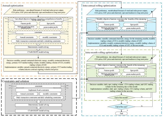
Figure 3.
Multi-stage rolling decision-making model.
First, conduct an annual optimization once at the beginning of the year, followed by intra-annual rolling optimizations within the year. The number of intra-annual rolling optimizations matching the number of months in the current year until year-end. After each monthly intra-annual rolling optimization, intra-month rolling optimizations are launched, with the number of optimizations matching the number of days in that month. Only after the current month ends will the monthly intra-annual rolling optimization for the next month proceed.
In the annual optimization stage, VPPs first solve the deterministic model of multi-level market transactions on an annual time scale based on the annual forecast of renewable energy outputs and market prices for the next year. Then, considering its own risk preference, it uses the objective function value of the deterministic model as a benchmark to solve the CVaR-EIGDT model of multi-level market transactions on an annual time scale, generating transaction plans and aggregated resource dispatching at the annual, monthly, daily, and hourly scales. The VPP implements the annual contracted electricity energy, the primary CET market trading volume, and the futures contract signing volume and price, before proceeding the intra-annual rolling optimization stage.
In the intra-annual rolling optimization stage, the VPP updates its forecasts for renewable energy outputs and market prices. It fixes the trading plans determined and implemented in the annual optimization stage, then solves a deterministic model for multi-level market trading with the remaining months of the year as the time scale. Subsequently, based on its risk preference, it uses the deterministic model’s objective function value as a benchmark to solve a CVaR-EIGDT model for multi-level market trading with the remaining months of the year as the time scale. This results in transaction plans and aggregated resource dispatching at the monthly, daily, and hourly scales. The VPP implements the monthly contracted electricity energy for the next month, as well as the monthly trading volume of the secondary CET market and GCT market for the next month, before proceeding the intra-month rolling optimization stage.
In the intra-month rolling optimization stage, the VPP continues to update its forecasts for renewable energy outputs and market prices. It fixes the trading plan determined and implemented in the intra-month rolling optimization stage, solves the deterministic model for multi-level market trading with the remaining days of the month as the time scale. Based on its risk preference, it uses the objective function value of the deterministic model, solves the CVaR-EIGDT model for multi-level market trading with the remaining days of the month as the time scale, generating trading plans and aggregated resource dispatching at various levels for each day and each hour. It implements the daily spot trading volume for the next day, as well as the trading volume in the secondary CET market and GCT market for the next day. This daily intra-month rolling process continues until the end of the month, when the VPP proceeds the next round of monthly intra-annual rolling optimization stage, repeating the cycle until the end of the year.
4.3. Model Solution
The proposed model constraints contain bilinear terms and if-then conditional constraints, which are linearized through binary expansion and the big M method, respectively.
The bilinear term formed by multiplying two continuous variables can be linearized using the binary expansion method [28]. Take for example, the reasonable value range for continuous variables is:
is expanded into discrete parameter values within its range. Let , then
is a 0–1 variable. Multiply both sides by and letting , then:
Additionally, supplementary constraints are as follows:
M is a sufficiently large constant. is linearized as (89)–(91).
The if-then conditional constraints can be linearized using the big M method [29]. Taking the Formula (82) as an example, it can be linearized as the following constraint conditions:
The linearized model is a mixed-integer linear programming problem, which can be solved by commercial solvers.
5. Case Study Analysis and Comparative Discussions
5.1. Case Introduction
To improve computational efficiency and facilitate presentation without compromising the universality of the results, a simulation is conducted using a condensed time scale: 4 typical months, 3 typical days per selected month, and 24 time periods per day. The peak load periods of the futures market are defined as 10:00 to 21:00 daily, with all remaining time periods designated as off-peak. The VPP under study is configured with one carbon capture unit, one wind power unit, one solar power unit, one energy storage unit, and one flexible load.
For the predicted renewable energy scenarios in annual, monthly, and daily decision-making, the mutual influence relationship between wind and solar renewable energy outputs needs to be considered [30]. This paper adopts the following method to generate combined wind and solar outputs scenarios: First, 100 independent wind and solar power output scenarios are generated via Latin hypercube sampling, using the latest forecast data as inputs. Subsequently, to capture the inherent correlation between wind and solar power outputs, the initial sampled scenarios are further resampled based on the Copula function, yielding 1000 joint wind–solar output scenarios along with their corresponding occurrence probabilities. To alleviate the computational burden caused by an excessive number of scenarios, the K-means clustering algorithm is employed to reduce the scenario set, ultimately deriving 5 typical scenarios and their respective probabilities. This method effectively reduces the computational complexity of the model while preserving the accuracy of characterizing renewable energy output uncertainty.
Given that flexible load is inherently adjustable, so load uncertainty is not considered in this paper. The annual forecast of wind and solar power outputs and the flexible load baseline in a certain region in southern China are shown in Figure 4.
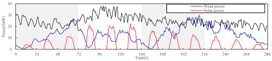
Figure 4.
Annual forecast of wind power, solar power, and flexible load baseline.
Spot market prices are obtained from the Guangdong Day-ahead Spot Market [31], while transaction prices in the primary and secondary CET market and the GCT market are derived from the National Carbon Emission Trading Market [32] and the China Green Power Certificates transaction platform [33], as shown in Figure 5.
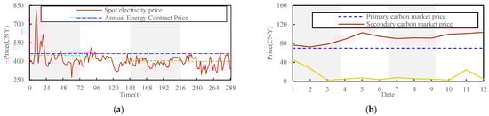
Figure 5.
Annual forecast of electricity and green market prices. (a) Electricity and green market prices forecast, (b) green market prices forecast.
Other market parameter settings are shown in Table 3.
Table 3.
Market Parameters.
δ = 0.1 and β = 0.1 in the CVaR-EIGDT robust model, and δ = −0.1 and β = 0.05 in the CVaR-EIGDT opportunity model. The simulation was computed on a personal computer with an Intel i7-10700K CPU and 64GB RAM, modeled by YALMIP in MATLAB 2023b, solved by Gurobi 12.0.1.
5.2. Analysis of Different Risk Decision
To analyze the differences in decision-making of VPPs under different risk preferences, this subsection compares the benefits and costs of the deterministic model, the multi-stage rolling robust model (abbreviated as robust model), and the multi-stage rolling opportunity model (abbreviated as opportunity model), as shown in Table 4.
Table 4.
Profits and costs of different decision-making models.
Compared to the deterministic model, the expected profits of the robust model and the opportunity model have changed by −11.4% and 7.9%, respectively. The opportunity model simultaneously captures the long-term price, futures contract price, and spot price differences in the multi-level electricity market, as well as the profit opportunities in the multi-level green market. The robust model sacrifices potential price arbitrage opportunities in exchange for a relatively conservative and risk-averse decision.
In terms of cost, compared to deterministic model, the robust model incurs higher dispatching costs to cope with the extremely adverse scenarios of uncertainties. Conversely, opportunity model utilizes the minimal incremental dispatching cost to address the extremely optimistic scenarios of uncertainties, thereby achieving a reduction in total cost.
Further analysis of VPP’s decision-making in multi-level electricity markets and multi-level green markets is shown in Table 5, Figure 6 and Figure 7, respectively.
Table 5.
Composition of power supply and electricity, and electricity market trading situation.
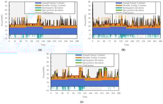
Figure 6.
Electricity market decision-making situation. (a) Robust model, (b) Opportunity model, (c) Deterministic model.
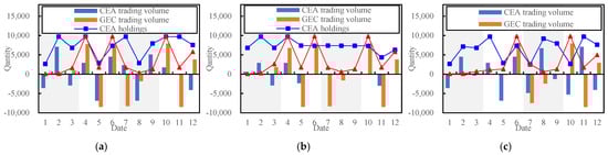
Figure 7.
Green market decision-making situation. (a) Deterministic model, (b) Robust model, (c) Opportunity model.
Compared with the deterministic model, the power generation of the carbon capture unit under the robust model and the opportunity model decreased by 3.5 MW·h and 1.2 MW·h, respectively, while the total output of wind and solar power registered respective changes of −11.4 MW·h and 12.9 MW·h. The reason is that the opportunity model reduces the power generation of carbon capture unit with higher costs in order to obtain higher profits, and increases the power generation of renewable energy sources with almost no cost but higher volatility; on the contrary, to ensure robustness, the robust model reduces the power generation of renewable energy sources, and at the same time, to avoid increasing the pressure of compliance obligation in the CET market, the output of carbon capture unit slightly decreases.
As Figure 6 shown, the deterministic model conducts spot deviation energy trading when there is a profitable spread between spot price and the medium- and long-term price. The robust model only conducts spot negative deviation trading when there is excess generation capacity in the first half of the year. The opportunity model conducts a large amount of spot negative deviation trading throughout the year.
Based on the analysis of Table 5 and Figure 6, compared with the deterministic model, the robust model considers the price risk of medium’ and long-term contracts, slightly reduces the volume of medium’ and long-term contracts to ensure long-term stable profit, and reduces the transaction of deviated energy in the high-risk spot market while decreasing the outputs of internal power sources to ensure sufficient reserve capacity, thereby ensuring the robustness of decision-making. The opportunity model has signed a large number of economical medium- and long-term contracts and conducts a large number of deviation settlements in the spot market to ensure the balance between its own power generation and marketed electricity energy under an aggressive market strategy.
As Figure 7 shown, all three models engage in CEAs and GECs trading during the compliance cycle, selling surplus CEAs and repurchasing GECs towards the end of the compliance cycle to fulfill their compliance obligation. The difference lies in that under the deterministic and opportunity models, VPP are actively trading in the secondary CET market and GCT market, pursuing the maximization of comprehensive profit through frequent transactions. In contrast, the scale of carbon trading under the robust model is significantly smaller. The main reason for this difference is that the characteristics of VPPs’ internal power generation resources determine that their pressure to fulfill CEAs compliance obligation is greater than that of GECs, and the price of CEAs is higher than that of GECs. The robust model tends to stabilize VPPs’ CEAs holdings through CEAs trading until the end of the compliance cycle, rather than engaging in market arbitrage. Therefore, under the premise of meeting expected profit requirements, it still trades in the GCT market with less compliance pressure to obtain certain profits. Conversely, the opportunity model actively captures arbitrage opportunities in the CET and GCT market on the basis of fulfilling compliance obligation, further enhancing overall profits.
The compliance completion status of VPP in the green market is shown in Table 6.
Table 6.
Compliance completion status in the green market.
There are significant differences in the green market fulfillment strategies of VPP under different risk preference. Under the deterministic model, more economical green market fulfillment strategies can be achieved through market transactions and offset mechanisms, without relying on carbon capture systems to cover additional emission reduction costs. The robust model, for the robustness of market decisions, extensively utilizes carbon capture systems while maintaining a certain surplus in the GCT market to ensure fulfillment in the case of unfavorable market prices. The opportunity model, on the other hand, coordinates the use of carbon capture systems and green market transactions under the most optimistic market prices to achieve the lowest-cost fulfillment strategy.
5.3. Analysis of Different Market Participation Situations
To show the advantages of VPP participation in the proposed multi-level coupled market, this paper sets up seven VPP market participation modes, as shown in Table 7.
Table 7.
Market participation modes.
The expected profits of VPP under different market participation modes is shown in Table 8.
Table 8.
Expected profits under different market participation modes.
The expected profits of M2 and M3 under the three models have decreased by an average of 18.2% and 19.2%, respectively compared to M1. The secondary CET market not only provides trading adjustments for CEAs but also provides VPPs the opportunity for additional profit. The GCT market, through the mechanism of using GECs to offset CEAs, alleviates the pressure on VPPs to fulfill their CEAs compliance obligation and similarly provides VPPs the ability to generate additional profit.
In terms of the profit of robust model, compared with M1, the average changes in the expected profit of M4, M5, M6, and M7 are −0.3%, −11.2%, 0.01%, and −1.5%, respectively. In terms of the profit of opportunity model, compared with M1, the average changes in the expected profits of M4, M5, M6, and M7 are −0.6%, −10.3%, −0.4%, and −8.5%, respectively.
Regardless of the risk preference, the medium- and long-term market is the “ballast stone” for VPP profits, which can ensure the continuous and stable profit of VPP and avoid the instability of profits caused by price fluctuations in the spot market. The futures market is a management tool for spot price risks. When losses are incurred due to spot price fluctuations in the settlement of spot deviations, delivery gains can be obtained in the futures market.
It is worth noting that in the robust model, the expected profit of M6 has a slight increase compared to that of M1. This is due to there is no need to face the risks of the spot market under the M6 mode, so the robust model can achieve a slightly higher expected profit. However, in the opportunity model, the expected profit decreases due to the loss of arbitrage opportunities in the spot market.
5.4. Analysis of Different Decision-Making Models
To verify the superiority of the proposed multi-stage rolling decision-making method based on CVaR-EIGDT, a comparative analysis was conducted between the proposed model and different decision-making models, as shown in Table 9. The two-stage rolling refers to the annual-daily two-stage rolling decision-making, without setting up a monthly trading plan for the green market, and monthly medium- and long-term contracts are signed on the first day of each month. In multi-stage SO, based on the three stages of annual-monthly-daily, we adopt the implementation method of a scenario tree of 1 × 5 × 5 and non-anticipativity constraints [34]. Rolling optimization in multi-stage SO is realized by fixing decisions for past time periods or stages.
Table 9.
Expected profits of different decision-making models.
As shown in Table 9, the expected profits of the CVaR-EIGDT robust model and CVaR-EIGDT opportunity model are the lowest and highest, respectively, except for the CVaR-IGDT models, while the expected profits of the EIGDT robust model and EIGDT opportunity model are the second lowest and second highest, respectively. It is due to CVaR-EIGDT taking into account risk management methods for both known and unknown probability of uncertainties, enabling it to capture both more adverse and more optimistic scenarios of uncertainties. Multi-stage SO models consider the adjustment of decisions in response to uncertainty scenarios, resulting in higher profits compared to the CVaR SO model, with both positioned in the middle range.
The expected profit of two-stage rolling decision-making is greater than that of multi-stage rolling decision-making, as the former does not consider long-term decisions in the monthly green market and only obtains optimal profits from a daily rolling perspective.
The proposed model is compared with the closest CVaR-IGDT model and the multi-stage SO model, as shown in Table 10.
Table 10.
Comparison of the proposed model with CVaR-IGDT model and multi-stage SO model.
As shown in Table 10, CVaR-EIGDT and CVaR-IGDT show little gap in expected profits, but there is a significant difference in the composition of specific profits, indicating that weights have influenced the decision-making. Specifically, the CVaR-IGDT-based model exhibits a larger gap in profits between the CET market and the GCT market, while the CVaR-EIGDT-based model achieves a more balanced performance in these markets. It is due to CVaR-IGDT assigning equal weighs to each uncertainty, leading to an overestimation of price volatility in the green market. Similarly, the CVaR-IGDT-based model underestimates the volatility of spot prices, resulting in lower futures profits compared to the CVaR-EIGDT model. CVaR-EIGDT, on the other hand, balances the weights of various uncertainties to make optimal decisions.
The significantly lower total cost compared to other models is the most distinctive feature of multi-stage SO. It is due to multi-stage SO considers the ability to adjust current decisions dynamically based on future uncertainty scenarios change, providing stronger resilience to uncertainty and reducing the total cost under uncertainties management. CVaR-EIGDT and CVaR-IGDT consider extreme price scenarios, resulting in relatively higher total costs.
Furthermore, based on the price fluctuation range and the generation method of wind–solar power joint output scenarios, four price scenarios are generated through random sampling for each price type, and 20 wind–solar power joint output scenarios are randomly sampled, resulting in a total of 44 × 20 = 5120 random scenarios. These random scenarios are substituted into the decision-making schemes of different models to verify their effectiveness in facing actual situations with uncertainties. The profit of different decision-making models in facing actual situations are shown in Figure 8.
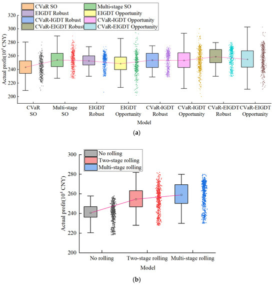
Figure 8.
Actual profits of different decision-making models. (a) Comparison of multi-stage rolling decision-making models, (b) comparison of CVaR-EIGDT robust model.
With the exception of the two SO models, opportunity models can capitalize on uncertainties to catch high profits, offering a wider range of profits, yet their average profits are lower than those of robust models. Owing to their inherent robustness, robust models exhibit a narrower profits range. The CVaR SO model achieves the lowest average profit, while the multi-stage SO model achieves a relatively higher average profit. However, as both remain within the SO framework, their robustness and opportunistic performance are inferior to those of the CVaR-EIGDT robust model and the opportunity model, respectively. The proposed CVaR-EIGDT model integrates the advantages of CVaR and entropy weight method, resulting in a wider range of profits compared to the pure IGDT model, while also achieving the highest average profits.
The no rolling model is unable to adjust decisions based on real-time information, resulting in lower average profits. Rolling decision-making can better adjust corresponding decisions based on updates of predictive information, thus achieving higher average profits. Multi-stage rolling decision-making achieves higher average profits than two-stage rolling decision-making. Compared to two-stage rolling decision-making, multi-stage rolling decision-making retains the real-time nature of rolling decision-making while adding the conservatism of monthly long-term decision-making, achieving an organic integration of dynamic decision adjustment and long-term decision planning.
5.5. Sensitivity Analysis on Risk Parameters δ and β
The key parameters controlling risk preferences in the IGDT and CVaR are the deviation parameter δ and the risk preference parameter β, respectively. The sensitivity analysis of the VPP’s expected profits under different values of δ and β is shown in Figure 9.
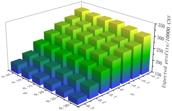
Figure 9.
Sensitivity of expected profits under different δ and β.
It can be seen that as δ and β increase, the expected profit decreases gradually, and the VPP’s risk attitude shifts from riskseeking to risk-averse. By dynamically adjusting δ and β, the VPP can achieve decisions with different risk preference and risk preference on different types of uncertainties.
5.6. Analysis of Linearization Efficiency
Table 11 compares the total solver time and expected profit before and after linearization.
Table 11.
Linearization efficiency.
It can be seen that linearization improves computational efficiency by 57.6% for the robust model and 12.6% for the opportunity model, with expected profit gap of only 0.19% and 0.37%.
5.7. Analysis of Applicability Across Different VPP Resource Scales
The applicability of the proposed model is tested on VPPs of different resource scales, as shown in Table 12.
Table 12.
Comparison for robust model with different resource scales.
It can be seen that the proposed model is adaptable to VPPs with different scales of resources, and the change in solver time is positively correlated with the change in schedulable resource scales.
5.8. Sensitivity Analysis of Different Regulatory Parameters
In the carbon markets of the EU and the U.S., free allocation of carbon allowances accounts for a smaller share, with greater reliance on auctions and market trading. Similarly, the proportion of renewable energy allowances in the green certificate markets of the EU and the U.S. is correspondingly higher. Therefore, significant modifications to the proposed model are unnecessary, only adjustments to key parameters is needed to simulate the European and U.S. market mechanisms to some extent. Table 13 presents a sensitivity analysis of different regulatory parameters.
Table 13.
Sensitivity analysis of different regulatory parameters in robust model.
It can be seen that under different regulatory parameter settings, the expected profits of the VPP can be maintained within a reasonable fluctuation range, which demonstrates the adaptability of the proposed model to diverse international market environments.
5.9. Analysis of Case for Annual Time Scales
The robust model was tested with annual time scales case, includes 12 months, 30 days per month, and 24 h per day. The results are shown in Table 14.
Table 14.
Annual time scale case testing on robust model.
It can be seen that the annual optimization and the first month of intra-annual rolling optimization and the first day of intra-month rolling optimization require longer computation time, while the average time is shorter. As the proposed model is an annual, monthly, and daily coordination model, its optimization process runs continuously throughout the year. The computing resources and time required for annual, monthly, and daily rolling optimization are all within an acceptable range.
5.10. Comparative Discussions with State-of-the-Art Methods
The decision-making methodological framework based on CVaR-EIGDT and multi-stage rolling proposed in this paper exhibits unique advantages in comparison with state-of-the-art methods in existing literature.
In comparison with multi-stage SO [34], this framework leverages the EIGDT to address price uncertainties characterized by unknown probability distributions, avoiding the modeling and computational burden incurred by complex scenarios trees and non-anticipativity constraints while providing direct protection against extreme price risks in multi-level coupled electricity market.
In contrast to advanced distributionally robust optimization [35], this framework does not rely on the construction of ambiguity sets that necessitate prior information or restrictive assumptions. Furthermore, this framework affords greater flexibility in risk preferences, and its entropy-weighted method for weight allocation affords a more objective measure of uncertainties.
Compared to artificial intelligence methods such as reinforcement learning [36], this framework can directly derive globally optimal solutions without requiring massive data or substantial computational resources for iterative training. Additionally, it features explicit market modeling, making the decision-making process more interpretable.
Furthermore, CVaR and EIGDT provide rigorous mathematical definitions and intuitive parameters for both risk-averse and risk-seeking preferences, allowing decision-makers to precisely control risk preferences. The multi-stage rolling decision-making method achieves deep temporal coupling of sequential decisions, dynamically adjusting decisions according to the updated information, thereby striking an optimal balance between long-term planning objectives and real-time adaptability.
The uniqueness of this method lies in the organic integration of CVaR, IGDT, entropy-weighted method, and multi-stage rolling decision-making. Characterized by low computational costs and modest requirements for uncertainty prediction accuracy, this framework provides a solution for complex decision-making problems involving both probability known and unknown uncertainties, as well as temporally coupled challenges, while featuring flexible risk preference parameters and high interpretability.
6. Conclusions
This paper focuses on the risk management of a multi-level coupled market where a VPP participates in both the electricity markets and green markets as an independent entity. It constructs a multi-level coupled market framework consisting of a “futures + medium- and long-term + spot” multi-level electricity market and a “primary CET+ secondary CET+ GCT” multi-level green market. To address the two uncertainties of known and unknown probability distributions of market prices and renewable energy output, as well as to achieve decision-making coordination across the time scales of multi-level coupled market, a general decision-making method based on CVaR-EIGDT risks management method and annual-monthly-daily coordinated multi-stage rolling method is proposed. On this basis, a Chinese case study was conducted, and the results show the following:
(1) The proposed multi-stage rolling risk decision-making method based on CVaR-EIGDT is enabled to make decisions with corresponding risk preferences in multi-level electricity markets and multi-level green markets under both robust and opportunity models. The robust model ensures that the decision does not fall below the set expected profit when uncertainties fluctuate, while the opportunity model seeks higher expected profits when uncertainties fluctuate. Adjusting the risk parameters can precisely achieve different risk preferences.
(2) The proposed multi-level coupled market framework involving VPPs can maximize the market profit of VPP. An exemplary Chinese case study shows that the medium- and long-term markets and electricity futures markets form a hedge against the renewable energy resources actual outputs and prices risks in markets; the primary and secondary CET market, as well as the GCT market, facilitate VPPs in achieving their low-carbon and green transformation goals while providing additional profit.
(3) Compared to multi-stage SO and other decision-making methods based on CVaR and IGDT, the proposed method exhibits stronger adaptability to real-world scenarios involving diverse uncertainties and achieves the highest average profit in practical scenario validation. The multi-stage rolling decision-making method, which balances real-time adjustments with long-term strategic planning, outperforms the two-stage rolling decision-making method in practical applications. In addition, compared to distributionally robust optimization and reinforcement learning methods, the proposed method offers unique strengths in terms of objectivity, flexibility in risk preferences, and interpretability.
(4) The proposed trading strategy decision-making method is a general methodological framework validated by China’s cases, featuring scalability across diverse application scenarios and time scales. Using China’s market framework as a case study, the model can be extended to VPP trading decisions in internationally multi-level coupled markets with diverse resource aggregation types by adjusting model parameters and the composition of VPP resources, demonstrating adaptability to international market environments. The VPP can make risk-preference-based decisions across simplified typical scenarios or even annual time scales with low computational costs, lower uncertainty prediction accuracy, and the coexistence of known and unknown probability distributions of uncertainties.
This paper still has certain limitations, which define the scope of the study but also point out directions for future research. First, it does not consider the impact of other market participants’ strategic behaviors and market clearing mechanisms on actual trading results. Second, it does not consider the network topology of VPP aggregated resources, and the VPP resource composition model was simplified without considering the detailed modeling of truly heterogeneous and unpredictable resources. Third, the model primarily focuses on market and production-side uncertainties, without incorporating real-world risks such as policy changes and component failures.
The above assumptions are necessary choices adopted in this study to focus on core decision-making methods rather than market clearing mechanisms and physical operational details, which clearly define the research scope of this paper, that is, the proposed model is suitable for evaluating the strategic value and economic potential of VPPs at the market level. Moreover, these assumptions can serve as a foundational starting point for more general future research, based on this study, the assumptions can be gradually relaxed by incorporating factors such as topology constraints, strategic bidding behavior, and multi-dimensional heterogeneous resource modeling and its uncertainties to further enhance the model’s practical applicability.
Author Contributions
Conceptualization, H.Z.; methodology, H.C.; software, H.Z.; validation, H.Z. and S.Z.; formal analysis, H.Z.; investigation, S.Z.; resources, H.C.; data curation, S.Z.; writing—original draft preparation, H.Z.; writing—review and editing, H.Z.; visualization, S.Z.; supervision, H.C.; project administration, H.C. All authors have read and agreed to the published version of the manuscript.
Funding
This research was funded by the National Key Research and Development Program of China (2022YFB2403500) and the National Natural Science Foundation of China (No. 51937005).
Data Availability Statement
Data available on request due to privacy. The data presented in this study are available on request from the corresponding author.
Conflicts of Interest
The authors declare no conflicts of interest.
References
- National Energy Administration. 2024 Annual Report on the Development of China’s Electricity Market. Available online: https://www.nea.gov.cn/20250717/54ae0fdb11f04b39a5b670999c04ef81/c.html (accessed on 5 December 2025).
- Development Report on China’s Green Electricity Certificates. 2024. Available online: https://www.nea.gov.cn/20250421/adcc933deed143dbbbfad982eacfc624/c.html (accessed on 10 October 2025).
- Progress Report of China’s National Carbon Market. 2025. Available online: https://www.mee.gov.cn/ywgz/ydqhbh/wsqtkz/202509/t20250927_1128352.shtml (accessed on 10 October 2025).
- Liu, W. Guangzhou Municipal Local Financial Supervision and Administration Bureau: Support the Guangzhou Futures Exchange in Advancing Carbon Futures Research. Futures Daily. 2024. Available online: https://link.cnki.net/doi/10.28619/n.cnki.nqhbr.2024.000321 (accessed on 11 November 2025). [CrossRef]
- Jiang, Y.; Chen, W. Review and Prospect of Coupled Electricity-Carbon-Renewable Portfolios Trading. Electr. Power Constr. 2023, 44, 1–13. [Google Scholar] [CrossRef]
- Tao, Y.; Wei, Z.; Lan, S.; Shi, S.; Su, P. Market-Wide Revenue Optimization Model of Power Generation Company Considering Electricity Futures Trading. Electr. Power Constr. 2024, 45, 141–149. [Google Scholar]
- Hongliang, W.; Benjie, L.; Daoxin, P.; Ling, W. Virtual Power Plant Participates in the Two-Level Decision-Making Optimization of Internal Purchase and Sale of Electricity and External Multi-Market. IEEE Access 2021, 9, 133625–133640. [Google Scholar] [CrossRef]
- Wu, Y.; Wu, J.; De, G. Research on Trading Optimization Model of Virtual Power Plant in Medium- and Long-Term Market. Energies 2022, 15, 759. [Google Scholar] [CrossRef]
- Liu, R.; Chen, K.; Sun, G.; Lin, S.; Jiang, C. Bidding Strategy for the Virtual Power Plant Based on Cooperative Game Participating in the Electricity-Carbon Joint Market. Int. J. Electr. Power Energy Syst. 2024, 163, 110325. [Google Scholar] [CrossRef]
- Zhou, Y.; Wu, J.; Sun, G.; Han, H.; Zang, H.; Wei, Z. A Two-Stage Robust Trading Strategy for Virtual Power Plant in Multi-Level Electricity-Carbon Market. Autom. Electr. Power Syst. 2024, 48, 1838–1846. [Google Scholar]
- Rockafellar, R.T.; Uryasev, S. Optimization of Conditional Value-at-Risk. J. Risk 2000, 2, 21–41. [Google Scholar] [CrossRef]
- Seyedeh-Barhagh, S.; Abapour, M.; Mohammadi-Ivatloo, B.; Shafie-Khah, M.; Laaksonen, H. Optimal Scheduling of a Microgrid Based on Renewable Resources and Demand Response Program Using Stochastic and IGDT-Based Approach. J. Energy Storage 2024, 86, 111306. [Google Scholar] [CrossRef]
- Khajehvand, M.; Fakharian, A.; Sedighizadeh, M. A Risk-Averse Decision Based on IGDT/Stochastic Approach for Smart Distribution Network Operation under Extreme Uncertainties. Appl. Soft Comput. 2021, 107, 107395. [Google Scholar] [CrossRef]
- Tan, Y.; Guan, L. Hybrid Optimization for Collaborative Bidding Strategy of Renewable Resources Aggregator in Day-Ahead Market Considering Competitors’ Strategies. Int. J. Electr. Power Energy Syst. 2023, 145, 108681. [Google Scholar] [CrossRef]
- Mirzaei, M.A.; Nazari-Heris, M.; Mohammadi-Ivatloo, B.; Zare, K.; Marzband, M.; Shafie-Khah, M.; Anvari-Moghaddam, A.; Catalão, J.P.S. Network-Constrained Joint Energy and Flexible Ramping Reserve Market Clearing of Power- and Heat-Based Energy Systems: A Two-Stage Hybrid IGDT–Stochastic Framework. IEEE Syst. J. 2021, 15, 1547–1556. [Google Scholar] [CrossRef]
- Aliasghari, P.; Mohammadi-Ivatloo, B.; Abapour, M. Risk-Based Scheduling Strategy for Electric Vehicle Aggregator Using Hybrid Stochastic/IGDT Approach. J. Clean. Prod. 2020, 248, 119270. [Google Scholar] [CrossRef]
- Huang, Y.; Li, T.; Yao, Y.; Ma, G.; Li, X.; Yu, X.; Xu, W.; Wang, J. IGDT-Based Two-Layer Optimization of Trading Strategies in Multi-Energy Markets. Energy 2025, 333, 137374. [Google Scholar] [CrossRef]
- Chen, L.; Xu, J.; Sun, Y.; Liao, S.; Ke, D.; Yao, L.; Mao, B. Bidding Strategies of Load Aggregators for Day-Ahead Market with Multiple Uncertainties. IEEE Trans. Power Syst. 2024, 39, 2786–2800. [Google Scholar] [CrossRef]
- Zhao, Y.; Liu, S.; Lin, Z.; Wen, F.; Yang, L.; Wang, Q. A Mixed CVaR-Based Stochastic Information Gap Approach for Building Optimal Offering Strategies of a CSP Plant in Electricity Markets. IEEE Access 2020, 8, 85772–85783. [Google Scholar] [CrossRef]
- Khaloie, H.; Vallee, F.; Lai, C.S.; Toubeau, J.-F.; Hatziargyriou, N. Day-Ahead and Intraday Dispatch of an Integrated Biomass-Concentrated Solar System: A Multi-Objective Risk-Controlling Approach. IEEE Trans. Power Syst. 2022, 37, 701–714. [Google Scholar] [CrossRef]
- National Development and Reform Commission Notice on Completing the Full Coverage of Renewable Energy Green Electricity Certificates and Promoting the Consumption of Renewable Energy Electricity. Available online: https://www.ndrc.gov.cn/xwdt/tzgg/202308/t20230803_1359093.html (accessed on 11 November 2025).
- Tian, Y.; Qin, Z.; Huang, Z. Day-Ahead Operational Strategy for Virtual Power Plant Considering Green Certificate Classification in Coupled Market. Electr. Power Constr. 2025, 46, 14–16. [Google Scholar]
- Lu, Z.; Huang, W. Overview of Global Electricity Futures Market and Analysis of Contract Characteristics. Secur. Futures China 2018, 23–27. [Google Scholar] [CrossRef]
- Biggins, F.A.V.; Ejeh, J.O.; Brown, S. Going, Going, Gone: Optimising the Bidding Strategy for an Energy Storage Aggregator and Its Value in Supporting Community Energy Storage. Energy Rep. 2022, 8, 10518–10532. [Google Scholar] [CrossRef]
- Ministry of Ecology and Environment. Notice on Completing the Allocation and Liquidation of National Carbon Emission Rights Trading Quotas for the Power Generation Industry in 2023 and 2024. Available online: https://www.gov.cn/zhengce/zhengceku/202410/content_6981938.htm (accessed on 29 May 2025).
- Wang, J.; Xu, J.; Wang, J.; Ke, D.; Liao, S.; Sun, Y.; Wu, Y. Bi-Level Stochastic Optimization for A Virtual Power Plant Participating in Energy and Reserve Market Based on Conditional Value at Risk. Power Syst. Technol. 2024, 48, 2502–2510. [Google Scholar] [CrossRef]
- Jianyuan, W.; Chengcheng, G.; Kechen, L. Anomaly Electricity Detection Method Based on Entropy Weight Method and Isolated Forest Algorithm. Front. Energy Res. 2022, 10, 984473. [Google Scholar] [CrossRef]
- Pereira, M.V.; Granville, S.; Fampa, M.H.C.; Dix, R.; Barroso, L.A. Strategic Bidding under Uncertainty: A Binary Expansion Approach. IEEE Trans. Power Syst. 2005, 20, 180–188. [Google Scholar] [CrossRef]
- Forrester, R.J.; Waddell, L.A. Modeling Using Logical Constraints. In Encyclopedia of Optimization; Pardalos, P.M., Prokopyev, O.A., Eds.; Springer International Publishing: Cham, Switzerland, 2023; pp. 1–5. ISBN 978-3-030-54621-2. [Google Scholar]
- Liang, Z.; Yin, X.; Chung, C.Y.; Rayeem, S.K.; Chen, X.; Yang, H. Managing Massive RES Integration in Hybrid Microgrids: A Data-Driven Quad-Level Approach with Adjustable Conservativeness. IEEE Trans. Ind. Inform. 2025, 21, 7698–7709. [Google Scholar] [CrossRef]
- Guangdong Power Exchange Center. Available online: https://pm.gd.csg.cn/portal/#/home (accessed on 6 November 2025).
- National Carbon Market Information Network. Available online: https://www.cets.org.cn/ (accessed on 6 November 2025).
- China Green Electricity Certificate Trading Platform. Available online: https://www.greenenergy.org.cn/ (accessed on 6 November 2025).
- Ding, T.; Hu, Y.; Bie, Z. Multi-Stage Stochastic Programming with Nonanticipativity Constraints for Expansion of Combined Power and Natural Gas Systems. IEEE Trans. Power Syst. 2018, 33, 317–328. [Google Scholar] [CrossRef]
- Wang, Y.; Huang, W.; Chen, H.; Yu, Z.; Hu, L.; Huang, Y. Optimal Scheduling Strategy for Virtual Power Plants with Aggregated User-Side Distributed Energy Storage and Photovoltaics Based on CVaR-Distributionally Robust Optimization. J. Energy Storage 2024, 86, 110770. [Google Scholar] [CrossRef]
- Wang, J.; Wu, J.; Kong, X. Multi-Agent Simulation for Strategic Bidding in Electricity Markets Using Reinforcement Learning. CSEE J. Power Energy Syst. 2023, 9, 1051–1065. [Google Scholar] [CrossRef]


Disclaimer/Publisher’s Note: The statements, opinions and data contained in all publications are solely those of the individual author(s) and contributor(s) and not of MDPI and/or the editor(s). MDPI and/or the editor(s) disclaim responsibility for any injury to people or property resulting from any ideas, methods, instructions or products referred to in the content. |
© 2025 by the authors. Licensee MDPI, Basel, Switzerland. This article is an open access article distributed under the terms and conditions of the Creative Commons Attribution (CC BY) license.