Optimal Design of Off-Grid Wind–Solar–Hydrogen Integrated Energy System Considering Power and Hydrogen Storage: A General Method

Abstract

Existing design methodologies for off-grid wind–solar–hydrogen integrated energy systems (WSH-IES) are typically case-specific and lack portability. This study aims to establish a unified design framework to enhance cross-scenario applicability while retaining case-specific adaptability. The proposed framework employs the superstructure concept, dividing the off-grid WSH-IES into three subsystems: energy production, conversion, and storage subsystems. The framework integrates equipment selection and capacity sizing into a unified optimization process described by a mixed-integer programming model. Additionally, the modular constraint template ensures generalizability across scenarios by linking the local resource protocol to the techno-economic parameters of the equipment, allowing the model to be adapted to various situations. The model was applied to two case studies. Economic analysis indicates that the pure electricity architecture is dominated by energy storage (battery costs account for 96.8%), while the hybrid architecture redistributes expenditures between batteries (67.8%) and electrolyzers (28.4%). It utilizes hydrogen as a complementary medium for long-duration energy storage, achieving cost risk diversification and enhanced resilience. Under current techno-economic conditions, real-time bidirectional electricity–hydrogen conversion offers no economic benefits. This framework quantifies cost drivers and design trade-offs for off-grid WSH-IES, providing an open modeling platform for academic research and planning applications.

1. Introduction

In recent years, environmental pollution and energy crisis have intensified, making energy transition an unavoidable global trend, particularly urgent for China [1,2,3]. This challenge is particularly acute for remote areas and islands where grid coverage is unavailable or unstable. These regions often rely on diesel generators, which are incompatible with decarbonization goals. In this context, the off-grid wind–solar–hydrogen integrated energy system (WSH-IES) emerges as a highly promising technological pathway. By integrating renewable generation with hydrogen energy storage technology, this system can manage intermittency through long-duration storage and directly supply hydrogen as a zero-carbon fuel, making it uniquely suited for modernizing remote energy supply.

Despite these technological advantages, the widespread deployment of WSH-IES faces the barrier of high heterogeneity. Remote islands and areas exhibit vastly diverse resource endowments and distinct load profiles. This case-specific variability renders rigid, predetermined system designs ineffective. Consequently, current design practices are predominantly case-by-case, relying heavily on expert experience.

The Energy Hub (EH) and Energy Bus (EB) concepts have been widely adopted as standardized theoretical frameworks for the systematic modeling of the coupling of multiple energy carriers, such as electricity, hydrogen, and heat [4,5]. The EH framework is an efficient modulator of multi-energy conversion via a unified coupling matrix [4]. However, it is inherently dependent on a fixed topology defined by the specific matrix structure. This rigidity restricts its application to the operation or sizing of predetermined systems. Conversely, the EB framework emphasizes nodal power balance, offering greater flexibility in describing network connections [6]. However, the absence of standardized conversion modules in EH-based models can lead to fragmentation when dealing with complex conversion technologies. Current literature rarely integrates these two strengths. The majority of studies utilize a static EH model to optimize sizing based on expert-defined, case-by-case topologies. This limitation restricts the design space to local optima.

Numerous studies have addressed the optimal sizing and operation of off-grid Hybrid Renewable Energy System (HRES) through diverse optimization techniques. Typical optimization approaches include mathematical programming methods, heuristic algorithms, and data-driven methods [7,8]. Heuristic or metaheuristic algorithms, such as Particle Swarm Optimization (PSO), Genetic Algorithms (GA), and other nature-inspired methods, are widely employed for system sizing due to their flexibility in handling nonlinear problems [9,10,11,12,13,14,15,16,17,18,19,20]. Although heuristic methods offer flexibility when handling non-convex problems, they have several drawbacks, including parameter sensitivity, unrepeatable results, and unguaranteed optimality. These limitations can be fatal for capital-intensive projects. Furthermore, to obtain a reasonable solution through computation, a sufficient number of experiments must be conducted to calculate the average value. This requires substantial computational resources and processing time. Conversely, mathematical programming methods (particularly Mixed-Integer Linear Programming, MILP) offer rigorous optimality guarantees [21,22]. However, to maintain computational tractability, conventional MILP applications are often confined to fixed system topologies. This limitation restricts the optimization scope, yielding solutions that are optimal only within a specific architecture, but potentially sub-optimal overall.

To bridge these gaps, this paper proposes a general and modular superstructure-based MILP framework for the optimal design of off-grid WSH-IES. The superstructure, originally developed for chemical process synthesis [23], integrates all feasible components and interconnections into a unified, comprehensive model. The integration of this topological flexibility with the standardized physics of the EH framework effectively decouples device physics from system logic. This approach enables the simultaneous optimization of topology, technology selection, and capacity, thereby facilitating the automatic synthesis of optimal, case-specific system blueprints that rigorously match local resource endowments and load profiles. Therefore, the clean energy system design and green hydrogen integration achieved by this framework directly align with the core objectives of the United Nations Sustainable Development Goals (SDGs), particularly SDG 7 (Affordable and Clean Energy) and SDG 13 (Climate Action).

In summary, the main work and contributions of this paper are as follows:

• First, a novel superstructure-based MILP framework was developed for the simultaneous optimization of topology, technology selection, and capacity in off-grid WSH-IES.
• Second, a modular modeling approach was developed to enhance adaptability and interpretability across diverse application scenarios.
• Third, comprehensive case studies demonstrated the framework’s effectiveness for different demand profiles (electricity-only and combined electricity–hydrogen).
• Finally, economic and sensitivity analysis provide insights into optimal configurations under a range of constraints and boundary conditions.

The remainder of this paper is organized as follows: The proposed methodology is detailed in Section 2. This includes the superstructure and the module modeling framework, the mathematical models of the candidate devices, and the MILP formulation. Section 3 describes the case studies and their associated input data. Section 4 presents the optimization results. Section 5 thoroughly discusses these findings and explores their implications. Finally, Section 6 concludes the paper and suggests directions for future research.

2. Methods

A mixed-integer programming optimization model based on the superstructure concept is illustrated in this section.

2.1. Superstructure and Modular Modeling Framework

The basic structure of the off-grid WSH-IES is shown in Figure 1. The concept of superstructure provides a comprehensive design space covering all technologically feasible configurations. In this framework, the off-grid WSH-IES can be classified into energy generation, conversion and storage subsystems. To navigate this space and identify the optimal system design, the problem is formulated as an MILP optimization model. The core idea is to integrate the technical and economic parameters of each type of equipment into a set of universal constraints. This enables the model to automatically select the types of equipment, determine their capacities, and schedule their operation in order to minimize the total annual cost, while ensuring that all physical and engineering constraints are satisfied. The following sections detail this modular modeling and optimization framework (depicted in Figure 2).

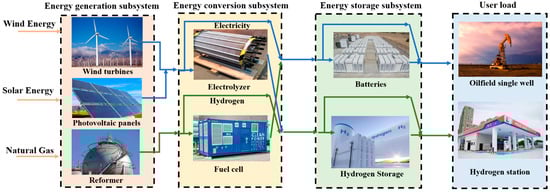
Figure 1. Superstructure for off-grid WSH-IES.

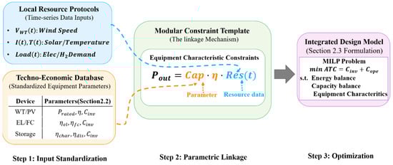
Figure 2. Modular modeling and optimization framework. In this diagram, connectors are distinguished by style and color: the blue dashed arrow on the left represents resource data flow input, the orange dashed arrow denotes equipment technical and economic parameter input, while the orange and blue dotted arrows at the bottom provide explanatory annotations.

2.2. Mathematical Model of Candidate Devices

The mathematical models of candidate devices include wind turbines [24], photovoltaics [25], reformers [26], electrolyzers [27], fuel cells [28], electricity storage [29,30], and hydrogen storage [31]. Specific models are detailed in Appendix A.

2.3. Mixed-Integer Linear Programming Formulation

The integrated design and operation optimization of the WSH-IES is formulated as an MILP problem based on the superstructure and device models. This problem arises from the fact that the decision variables include both continuous variables (e.g., power flows and storage levels) and integer variables (e.g., equipment selection and quantities). The MILP framework is chosen because it rigorously handles such discrete-continuous combinatorial problems and guarantees global optimality within a defined optimality gap. The model consists of the following components.

2.3.1. Decision Variables

Decision variables are primarily categorized into design variables and operational variables. Design variables determine topology and capacity, while operational variables dictate scheduling. Design variables include equipment selection parameters and quantity of equipment, whereas operational variables represent the input and output power of conversion equipment and the storage capacity of energy storage devices.

2.3.2. Objective Function

To evaluate economic cost, the Annual Total Cost (ATC) is adopted as the design objective function [22], which comprises the annual equipment purchase and installation costs ($C_{\mathrm{i}\mathrm{n}\mathrm{v}}$), the operation and maintenance cost ($C_{\mathrm{o}\mathrm{p}\mathrm{e}}$), and the fuel consumption cost ($C_{\mathrm{f}\mathrm{u}\mathrm{e}\mathrm{l}}$). The ATC is formulated as follows:

$$\mathrm{m}\mathrm{i}\mathrm{n}\mathrm{A}\mathrm{T}\mathrm{C}=C_{\mathrm{i}\mathrm{n}\mathrm{v}}+C_{\mathrm{o}\mathrm{p}\mathrm{e}}+C_{\mathrm{f}\mathrm{u}\mathrm{e}\mathrm{l}}+C_{\mathrm{p}\mathrm{e}\mathrm{n}}$$

(1)

$$C_{\mathrm{i}\mathrm{n}\mathrm{v}}=\sum _{i\in I}\sum _{j\in J}{q}_{i,j}·x_{i,j}·{\lambda }_{i,j}·R_{i,j}$$

(2)

$$C_{\mathrm{o}\mathrm{p}\mathrm{e}}=\sum _{i\in I}\sum _{j\in J}{c}_{i,j}·x_{i,j}·{\lambda }_{i,j}$$

(3)

$$C_{\mathrm{f}\mathrm{u}\mathrm{e}\mathrm{l}}=\sum _{t\in T}\sum _{i\in I}{c}_{\mathrm{f}\mathrm{u}\mathrm{e}\mathrm{l},i}·P_{i,t}^{in}$$

(4)

$$C_{\mathrm{p}\mathrm{e}\mathrm{n}}=\sum _{t\in T}\sum _{c\in C}{c}_{\mathrm{p}\mathrm{e}\mathrm{n},i}·P_{c,t}^{loss}$$

(5)

$$R_{i,j}=r{\left(1+r\right)}^{L_{i,j}}/[{(1+r)}^{L_{i,j}}-1]$$

(6)

where $C_{\mathrm{i}\mathrm{n}\mathrm{v}}$ refers to the annual equipment purchase and installation costs; $C_{\mathrm{o}\mathrm{p}\mathrm{e}}$ refers to the annual operation and maintenance costs; $C_{\mathrm{f}\mathrm{u}\mathrm{e}\mathrm{l}}$ refers to the fuel expense; $C_{\mathrm{p}\mathrm{e}\mathrm{n}}$ refers to the penalty expense; $R_{i,j}$ refers to the capital recovery factor; $q_{i,j}$ stands for the purchase cost of a single unit of equipment, CNY/unit; $x_{i,j}$ stands for the number of the type $j$ of equipment of category $i$; ${\lambda }_{i,j}$ stands for 0–1 integer variable, indicating whether the category and type of equipment are installed or not; $r$ is the discount rate of the equipment, which is set to 0.08 in this paper; $L_{i,j}$ is the life of the equipment model (years); $c_{i,j}$ is the annual operation and maintenance cost of the system equipment, CNY/year; $c_{\mathrm{f}\mathrm{u}\mathrm{e}\mathrm{l},i}$ is the unit price of fuel, CNY/Nm³; $P_{i,t}^{in}$ stands for the consumption of fuel $;P_{c,t}^{loss}$ represents the value of load loss; $T$ stands for the time period; $I$ is the set of technology types; $J$ stands for the set of candidate models; $C$ stands for the set of energy carriers.

2.3.3. Constraints

The optimization model incorporates the following constraints to ensure technical feasibility, operational limits, and system-level requirements in the design of integrated energy systems. Constraints can be categorized into four primary types: configuration logic constraints, component physical constraints, network balancing constraints, and boundary and security constraints.

• Mutually Exclusive Selection

This constraint enforces standardization in maintenance and operation by allowing at most one technology model to be selected within each category $i\in I$. It is formulated as

$$\sum _{j=1}^J{\lambda }_{i,j}\le 1,i\in I$$

(7)

where ${\lambda }_{i,j}$ is a 0–1 integer variable; ${\lambda }_{i,j}=1$ indicates that $j$ type of $i$ category is selected, and ${\lambda }_{i,j}=0$ indicates that the type is not selected.

• Capacity-Selection Coupling (Big-M Logic)

To logically link the installed capacity variable $x_{i,j}$ with the technology selection variable ${\lambda }_{i,j}$, the following Big-M constraints are introduced:

$$x_{i,j}\le M\cdot {\lambda }_{i,j}\forall i\in I,\forall j\in J$$

(8)

$$x_{i,j}\ge {\lambda }_{i,j}\forall i\in I,\forall j\in J$$

(9)

Here, $M$ is a sufficiently large constant. These constraints ensure that capacity is positive only if the corresponding technology is selected, and that selection forces a minimum capacity.

• Generalized Output Limits (Generator & Converter)

For generators and converters ($\forall i\in I_{gen}\cup I_{con}$), the output power $P_{i,j,t}^{out}$ is bounded by the installed capacity and the real-time availability factor ${\varphi }_{i,t}$:

$$0\le P_{i,j,t}^{out}\le x_{i,j}\cdot Ca{p}_{i,j}^{rated}\cdot {\varphi }_{i,t},\forall i\in I_{gen}\cup I_{con}$$

(10)

where ${\varphi }_{i,t}$ is the normalized resource profile (e.g., for wind or solar) or equals 1 for dispatchable units.

• Input–Output Conversion Law (Coupling Physics)

For energy conversion devices ($i\in I_{con}$), the output is related to the input via the conversion efficiency ${\eta }_{i,j}:$

$$P_{i,j,t}^{out}=P_{i,j,t}^{in}\cdot {\eta }_{i,j},\forall i\in I_{con}$$

(11)

• Storage State Dynamics

The state of charge $S_{i,j,t}$ for storage devices ($i\in I_{sto}$) evolves according to

$$S_{i,j,t}=S_{i,j,t-1}\cdot \left(1-{\delta }_i\right)+P_{i,j,t}^{in}\cdot {\eta }_{i,j}^{ch}-P_{i,j,t}^{out}/{\eta }_{i,j}^{dis},\forall i\in I_{sto}$$

(12)

where ${\delta }_i$ is the self-discharge rate, and ${\eta }_{i,j}^{ch/dis}$ are charging/discharging efficiency.

• Storage Technical Limits

Storage operation is subject to

$$\left(1-{DOD}_i\right)\cdot x_{i,j}\cdot Ca{p}_{i,j}\le S_{i,j,t}\le x_{i,j}\cdot Ca{p}_{i,j}$$

(13)

$$P_{i,j,t}^{in/out}\le x_{i,j}\cdot P_{i,j}^{rate\_max}$$

(14)

These ensure that the state of charge remains within depth-of-discharge limits and that charge/discharge rates do not exceed rated power.

• Energy balance constraints

For each energy carrier $c$ (e.g., Electricity, Hydrogen), the sum of inflows must equal the sum of outflows at every time step.

$$\sum _{i\in I}\sum _{j\in J}{P}_{i,j,t}^{out}\cdot {\theta }_{i,c}^{out}+P_{c,t}^{loss}={Load}_{c,t}+\sum _{i\in I}\sum _{j\in J}{P}_{i,j,t}^{in}\cdot {\theta }_{i,c}^{in}+P_{c,t}^{curt}$$

(15)

where ${\theta }_{i,c}^{in/out}\in \left\{\mathrm{0,1}\right\}$ is the incidence matrix mapping devices to buses.

• Off-grid Cyclic Stability

For isolated systems, storage levels at the end of the horizon must equal initial levels to ensure sustainability:

$$S_{i,j,T}{=S}_{i,j,T},\forall i\in I_{sto}$$

(16)

• Environmental Constraints (Optional)

A cumulative emission limit can be imposed:

$$\sum _{t\in T}\sum _{i\in I}{E}_{\mathrm{f}\mathrm{a}\mathrm{c}\mathrm{t}\mathrm{o}\mathrm{r},i}\cdot P_{i,t}^{out}\le E_{\mathrm{l}\mathrm{i}\mathrm{m}\mathrm{i}\mathrm{t}}^{CO2}$$

(17)

where $E_{\mathrm{f}\mathrm{a}\mathrm{c}\mathrm{t}\mathrm{o}\mathrm{r},i}$ is the emission factor of device $i$. The operation of reformer generates carbon dioxide emissions. To establish a zero-carbon system, the allowable carbon dioxide emissions here are set to zero.

2.3.4. Model Linear Strategy

To ensure computational tractability and reliable convergence, the nonlinearities in the original model are addressed by strategic linearization. The primary nonlinearities include the cubic wind turbine power curve and bilinear terms arising from products of binary selection variables and continuous energy flows. We apply the following linearization techniques:

(a)

Piecewise Linear Approximation (PWL): This method converts non-linear relationships into a set of linear constraints to ensure that the maximum approximation error remains below 1.5%.

(b)

Big-M Method: This is a standard reformulation technique in MILP that enforces conditional logic without introducing nonlinearity. It is used to precisely linearize the product of binary variables and continuous variables.

2.4. Model Implementation, Solution and Validation

The implementation of the MILP model was done in Python 3.12, and the COPT solver 7.2.11 was used to solve it. The COPT solver is a high-performance commercial solver for linear and mixed-integer programming. COPT uses advanced algorithms, such as branch-and-bound and cutting-plane methods, to find optimal solutions. For all of the case studies presented in this paper, the solver was configured to terminate when the optimality gap fell below 0.1%, thereby ensuring the practicality of the solutions from an engineering standpoint.

2.5. Boundary Conditions and Demonstrability Analysis

Boundary conditions define the external limits and specific stakeholder requirements for system design. In addition to physical boundaries such as resource availability and land area, demonstrability is a critical non-technical boundary condition for prototype or demonstration projects. Demonstrability reflects the requirement to select technologies that highlight innovation, reliability, and future scalability to attract investment and policy support.

Within our optimization framework, demonstrability is quantified and incorporated through two approaches: expanding the set of technology candidates and conducting multi-objective scenario analysis. The system can explore trade-offs between cost and technological maturity by covering conventional and emerging technologies through the equipment database. Scenario analysis is also used to evaluate a technology’s demonstrability. For example, in Section 3, we defined multiple scenarios where specific technologies (such as wind turbines) are included as part of the configuration scheme. By comparing these scenarios, we can evaluate the impact of demonstrability requirements on system configurations and their economic viability.

3. Case Study

3.1. Basic Data

Two cases have been conducted to illustrate the modeling and optimization framework for designing the WSH-IES. The targeted energy consumers are the Pipeline Bureau’s Subordinate units and the hydrogen refueling station. The former energy consumer only demands electricity, while the latter demands both electricity and hydrogen. The required inputs for the design optimization model are the meteorological resource information, demand data, and the techno-economic parameters of the equipment.

3.1.1. Meteorological Resource Data

The meteorological resource data used in this paper provides insights into the distribution of wind speed, solar radiation intensity, and ambient outdoor temperatures for a typical year in that area, as depicted in Figure 3. Clearly, this area is rich in solar resources but lacks wind resources. The solar radiation data imply that hourly fluctuations are strong for morning and late afternoon but weak around solar noon.

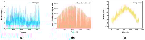
Figure 3. Meteorological resource data in the case city. (a) Wind speed; (b) Solar radiation intensity; (c) Temperature.

3.1.2. Demands

For simplification, the demands are not subject to seasonality, and the hourly demand on a representative day is shown in Figure 4. Figure 4 presents the electricity load and hydrogen load over 24 h for two cases. In Case 1, the electricity load fluctuates between 7 kW and 14 kW, while there is no demand for the hydrogen load. In Case 2, both the electricity load and hydrogen load remain relatively stable, with the electricity load at 10 kW and the hydrogen load at 16 Nm³. Note that the electricity unit is kilowatt (kW), while the hydrogen unit is Nm³, and the natural gas price is set to 3.95 CNY/Nm³.

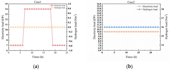
Figure 4. Load demands for cases 1 and 2. (a) Case 1: the electricity load fluctuates between 7 kW and 14 kW, while there is no demand for hydrogen load; (b) Case 2: both the electricity load and hydrogen load remain relatively stable, with the electricity load at 10 kW and the hydrogen load at 16 Nm³.

3.1.3. Technological and Economic Data

The classification of equipment types in this study is based solely on differences in capacity and techno-economic parameters, such as energy efficiency, unit investment cost, operation and maintenance (O&M) cost, and lifetime of each technology, detailed in Table 1, Table 2 and Table 3. These types do not represent fundamental technical differences but rather variations in the scale and cost-effectiveness of the equipment. For instance, wind turbines of different types (e.g., Type a, Type b, Type c) will have distinct power ratings, investment costs, and O&M costs. These differences may impact the final configuration results and enable the model to evaluate trade-offs between cost and performance.

Table 1. Techno-economic parameters of the energy generation technologies.

Technologies	Type *	Investment Cost, CNY/Unit	O&M Cost, CNY/Unit	Capacity, kW (or Nm3/h)	Lifetime, Year	Tech-Specific Parameter 1	Tech-Specific Parameter 2	Tech-Specific Parameter 3
WT	a	55,800	750	5	25	${\mathrm{V}}_{\mathrm{r}\mathrm{a}\mathrm{t}\mathrm{e}\mathrm{d}}:$ 11 m/s	${\mathrm{V}}_{\mathrm{i}\mathrm{n}}:$2.5 m/s	${\mathrm{V}}_{\mathrm{o}\mathrm{u}\mathrm{t}}:$25 m/s
	b	97,400	750	10	25	${\mathrm{V}}_{\mathrm{r}\mathrm{a}\mathrm{t}\mathrm{e}\mathrm{d}}:$ 11 m/s	${\mathrm{V}}_{\mathrm{i}\mathrm{n}}:$2.5 m/s	${\mathrm{V}}_{\mathrm{o}\mathrm{u}\mathrm{t}}:$25 m/s
	c	194,500	750	20	25	${\mathrm{V}}_{\mathrm{r}\mathrm{a}\mathrm{t}\mathrm{e}\mathrm{d}}:$ 11 m/s	${\mathrm{V}}_{\mathrm{i}\mathrm{n}}:$2.5 m/s	${\mathrm{V}}_{\mathrm{o}\mathrm{u}\mathrm{t}}:$25 m/s
PV	a	750	50	0.55	25	${\mathrm{I}}_{\mathrm{s}\mathrm{t}\mathrm{d}}:$ 1000 W/m2	β: 0.0045 K−1	${\mathrm{T}}_{\mathrm{s}\mathrm{t}\mathrm{d}}:$25 °C
	b	5600	370	200	25	${\mathrm{I}}_{\mathrm{s}\mathrm{t}\mathrm{d}}:$ 1000 W/m2	β: 0.0045 K−1	${\mathrm{T}}_{\mathrm{s}\mathrm{t}\mathrm{d}}:$25 °C
RH	a	50,000	10,000	1	10	Efficiency: 0.98	Water consumption: 0.9 L/Nm3	$\mathrm{Wd}:3\mathrm{k}\mathrm{W}\mathrm{h}/\mathrm{N}{\mathrm{m}}^3$

* “Type a”, “Type b”, and “Type c” represent different equipment models distinguished only by their capacity and techno-economic parameters (e.g., investment cost, O&M cost). They do not indicate fundamental technical differences. Vin m/s: Cut-in wind speed; β, K⁻¹: Shape parameter of the PV; water, L/Nm³: Water consumption for electrolytic hydrogen production; capacity (kW or Nm³/h): Rated capacity of the equipment.

Table 2. Techno-economic parameters of the energy conversion technologies.

Technologies	Type	Investment Cost, CNY/Unit	O&M Cost, CNY/Unit	Capacity, kW (or Nm3/h)	Lifetime, Year	Efficiency	$\mathbf{Water},\mathbf{L}/\mathbf{N}{\mathbf{m}}^3$	$\mathbf{Wd},\mathbf{k}\mathbf{W}\mathbf{h}/\mathbf{N}{\mathbf{m}}^3$
EL	a	450,000	10,000	2	10	0.85	0.9	4.8
FC	a	50,000	3333	5	10	0.55	-	-

Table 3. Techno-economic parameters of the energy storage technologies.

Technologies	Type	Investment Cost, CNY/Unit	O&M Cost, CNY/Unit	Capacity, kW (or Nm3/h)	Lifetime, Year	Efficiency
BT	a	1200	6	1	10	0.9
HS	a	50,000	3333	5	10	3

3.2. Solving Strategy

The model is formulated in Python and calculated with the COPT Optimizer. The solving strategy is shown in Figure 5.

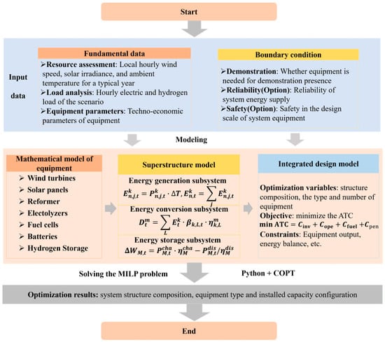
Figure 5. Optimization flowchart for the proposed system.

(a)

Initialize necessary parameters, such as local meteorological parameters, techno-economic parameters of candidate equipment. Determine the electricity and hydrogen loads and the boundary condition.

(b)

Establish the mathematical model of the candidate equipment.

(c)

Establish the “structure-type-capacity” integrated design optimization model based on the unit models established in (b).

(d)

Solve the model established in (c) by Python and COPT.

3.3. Setting of Scenarios

In this study, six scenarios are designed to evaluate the model’s effectiveness and analyze the impact of equipment demonstration on system design and economic performance. Equipment demonstration in this context involves the inclusion of specific components, such as wind turbines, electroliers, and hydrogen storage tanks, to simulate practical implementation scenarios and analyze their influence on system outcomes. The incorporation of such components adds additional constraints or increased costs in the selection process, representing potential future implementation. It is imperative to acknowledge that, in response to the dual carbon policy, this study explores the configuration of zero-carbon systems, where carbon emissions are managed to a net zero level.

These scenarios are summarized in Table 4. Scenario 1 represents the system designed for Case 1, serving the Pipeline Bureau’s Subordinate units, without considering the boundary conditions. Scenario 2 also pertains to Case 1 but includes wind turbines, electrolyzers, and hydrogen storage tanks. This scenario is used to assess how these components affect the system’s design and economic performance when additional equipment is introduced. Scenario 3 is designed for Case 2, targeting the hydrogen refueling station without equipment demonstration. Scenario 4 addresses Case 2, incorporating the demonstration of equipment like wind turbines. Scenario 5 represents a system for case 2 that excludes both electro-hydrogen coupling and equipment demonstration. Scenario 6 is similar to Scenario 5 but includes the demonstration of the equipment, such as wind turbines, photovoltaic, and reformer hydrogen plants.

Table 4. Scenario configurations for analyzing the impacts of electro-hydrogen coupling and boundary conditions.

	Scenario 1	Scenario 2	Scenario 3	Scenario 4	Scenario 5	Scenario 6
Cases	1	1	2	2	2	2
Electro-hydrogen coupling	√ *	√	√	√	-	-
Boundary conditions	- *	√	-	√	-	√

* Note: “√” indicates that the condition is considered, while “-” indicates that it is not considered.

4. Results

4.1. Optimal System Configurations

The optimization results for two distinct cases are summarized below.

4.1.1. Electricity-Only Load

The optimization results for Case 1 (electricity-only demand) are summarized in Table 5. In Scenario 1, only photovoltaic panels and lithium batteries are selected to meet the electricity demand, and there is no hydrogen-related equipment is included. When a technology demonstrability is enforced in Scenario 2, the system cost increases. This is because it requires the inclusion of a wind turbine, electrolyzer, fuel cell, and hydrogen storage for demonstration purposes. The total annual cost rises from 113,555.46 CNY to 195,856.70 CNY, an increase of approximately 72.5%. This increase is primarily due to the addition of unused demonstration equipment, such as a 5 kW wind turbine and a 2 Nm³/h electrolyzer, which are not economically justified by the load profile alone. This finding illustrates the cost increase associated with non-economic design constraints, such as technology demonstration.

Table 5. Optimal equipment capacities and costs for Case 1.

Devices	Scenario 1			Scenario 2
	Type	Units	Capacities *	Type	Units	Capacities
WT (kW)	-	0	0	a	1	5
PV (kW)	b	4	800	a	b	1000
RH (${\mathrm{N}\mathrm{m}}^3/\mathrm{h}$)	-	0	0	-	0	0
EL (${\mathrm{N}\mathrm{m}}^3/\mathrm{h}$)	-	0	0	a	1	2
FC (kW)	-	0	0	a	1	5
BT (kWh)	a	595	595	a	467	467
HS (${\mathrm{N}\mathrm{m}}^3$)	-	-	-	a	1	55.617
Annual total cost (CNY)	113,555.46			195,856.7

* Note: Capacities are the product of the unit capacity of the selected equipment model and the number of units.

4.1.2. Combined Electricity–Hydrogen Load

For the hydrogen refueling station with combined electricity and hydrogen demand, the optimization results are detailed in Table 6 and Table 7. In Scenario 3 (with electro-hydrogen coupling), the model selects a high-capacity PV system (Type b, 2400 kW), an electrolyzer array (10 units of Type a, totaling 20 Nm³/h), hydrogen storage, and a large battery bank. The configuration favors a single, large PV unit over multiple smaller ones, indicating that economies of scale outweigh the flexibility benefits of modular units for this centralized demand profile. Scenarios 4, 5, and 6 explore variations with and without coupling and demonstrability constraints, showing relatively stable PV and electrolyzer capacities but variations in other components (e.g., fuel cell inclusion) and associated costs.

Table 6. Optimal equipment capacities for Case 2 with electro-hydrogen coupling.

Devices	Scenario 3			Scenario 4
	Type	Units	Capacities	Type	Units	Capacities
WT (kW)	-	0	0	a	1	5
PV (kW)	b	12	2400	b	12	2400
RH (${\mathrm{N}\mathrm{m}}^3/\mathrm{h}$)	-	0	0	-	0	0
EL (${\mathrm{N}\mathrm{m}}^3/\mathrm{h}$)	a	10	20	a	10	20
FC (kW)	-	0	0	a	1	5
BT (kWh)	a	1750	1750	a	1747	1747
HS (${\mathrm{N}\mathrm{m}}^3$)	a	3	166.85	a	3	166.85
Annual total cost (CNY)	1,137,183.26			1,153,846.58

Table 7. Optimal equipment capacities for Case 2 without electro-hydrogen coupling.

Devices	Scenario 5			Scenario 6
	Type	Units	Capacities	Type	Units	Capacities
WT (kW)	-	0	0	a	1	5
PV (kW)	b	12	2400	b	12	2400
RH (${\mathrm{N}\mathrm{m}}^3/\mathrm{h}$)	-	0	0	-	0	0
EL (${\mathrm{N}\mathrm{m}}^3/\mathrm{h}$)	a	10	20	a	10	20
FC (kW)	-	0	0	-	0	0
BT (kWh)	a	1750	1750	a	1747	1747
HS (${\mathrm{N}\mathrm{m}}^3$)	a	3	166.85	a	3	166.85
Annual total cost (CNY)	1,137,183.26			1,143,062.11

4.2. Economic Performance Analysis

4.2.1. Impact of Equipment Demonstrability

Imposing demonstrability constraints that require the inclusion of specific equipment, such as wind turbines and electrolyzers, leads to a measurable increase in costs across all cases. In Case 1, this constraint increases the ATC by 72.5%, demonstrating that hydrogen equipment is economically suboptimal for pure electrical loads. The cost premium arises from the capital and maintenance costs of demonstration assets with very low utilization. In contrast, for the large-scale hybrid system in Case 2, adding a single demonstration wind turbine results in a marginal ATC increase of only 0.22–0.52%. This indicates that the economic impact of non-optimal demonstration equipment is significantly diluted in larger, more complex systems, though it does not imply the equipment itself is cost-effective.

4.2.2. Impact of Electro-Hydrogen Coupling

As shown in Table 6 and Table 7, scenarios allowing for electro-hydrogen coupling (Scenario 3) and prohibiting coupling (Scenario 5) demonstrate equivalent system configurations and ATC. This seemingly contradictory outcome reveals a critical economic and technical trade-off inherent in this system design. In off-grid scenarios, electrolyzers primarily undertake continuous hydrogen supply tasks, with their operational periods already approaching saturation. Theoretically, coupling mechanisms could convert surplus electricity into hydrogen storage, thereby reducing reliance on battery energy storage. However, optimization results indicate that the cost of reconverting stored hydrogen back into electricity via fuel cells exceeds the expenses of increasing battery capacity or tolerating minor curtailment. Consequently, the model rationally excludes fuel cell deployment, rendering bidirectional electricity–hydrogen coupling unfeasible at the equipment level.

4.2.3. Analysis of Key Cost Components

Figure 6 compares the annual total cost composition of two typical systems, revealing their fundamental economic structural differences. Figure 6 shows that costs in pure power systems are highly concentrated: batteries account for 96.8%, while PV contributes only 3.2%, making energy storage the absolute dominant factor. After introducing hydrogen loads, the battery share drops to 67.8%, electrolyzers rise to 28.4%, and other components account for negligible proportions. The hydrogen chain shoulders long-duration storage, while batteries remain dominant for short-term regulation. The cost structure shifts from single-directional to bidirectional electricity–hydrogen integration, enhancing the system’s resilience against risks.

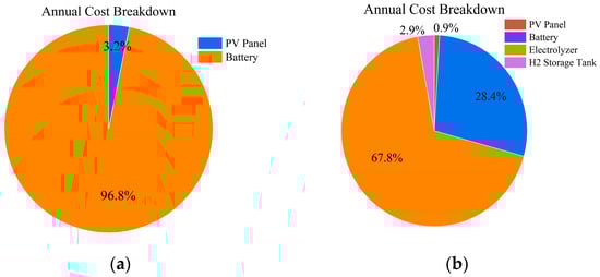
Figure 6. Annual Total Cost Composition for Scenario 1 and 3. (a) Scenario 1: Electricity-only load; (b) Scenario 3: Combined electricity–hydrogen load. Percentages indicate the contribution of each component’s ATC to the total system’s ATC.

4.3. Sensitivity Analysis

To assess the robustness of key equipment capacity parameters to system economics, we conducted a univariate sensitivity analysis on the optimized baseline system. The analysis calculated the percentage increase in the system’s ATC when the capacities of PV, battery storage, electrolyzer, and hydrogen storage tank deviated by ±30% from their optimal values. The results are shown in Figure 7.

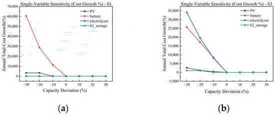
Figure 7. Impact of equipment capacity deviations on the annual total cost growth in (a) Scenario 1 and (b) Scenario 3.

In Figure 7, the cost of the pure power system (a) exhibits extreme sensitivity to battery capacity fluctuations of ±30%, displaying a steep slope. The impact of the PV system is one order of magnitude lower, while the hydrogen equipment shows no effect. This observation corresponds with the cost structure, where batteries constitute 97% of the total cost. After the introduction of the hydrogen chain (b), capacity fluctuations in all four equipment types have a marked impact on total costs. Battery sensitivity decreases, while the sensitivities to PV and electrolyzers increase, and hydrogen storage also plays a significant role. The system thus transitions from unidirectional vulnerability to a bidirectionally balanced state, achieving risk dispersion and enhanced resilience.

4.4. Seasonal Impact Analysis

To assess the impact of seasonal fluctuations in load and resource availability on system design, this study introduces the Seasonality Amplitude Factor as a key parameter. Its value ranges from 0 (no seasonality) to 1 (strong seasonality), simulating scenarios from uniform load distribution to significant peak-to-trough variations. Figure 8 illustrates the trends in total system cost and optimal configuration of key equipment as this factor varies.

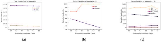
Figure 8. Variation in system cost and optimal equipment configuration with seasonality amplitude factor for two typical scenarios. (a) Total system cost for Scenario 1 (S1) and Scenario 3 (S3); (b) optimal equipment capacity for Scenario 1; (c) optimal equipment capacity for Scenario 3.

Figure 8a reveals a key finding. The total system cost exhibits an overall downward trend as seasonal fluctuations intensify. This phenomenon contradicts the intuitive assumption that increased volatility would raise costs. Seasonal amplification concentrates peak loads during periods of high output from renewable energy sources, particularly photovoltaic systems. For the off-grid systems studied here, this means abundant daytime solar energy can directly meet larger peak loads. Consequently, reliance on costly energy storage (battery discharge) is significantly reduced. This leads to more economical overall capacity configuration and operational strategies, ultimately reflected in lower annualized total costs.

The experiment compared optimal equipment capacity configurations for two scenarios (S1 and S3) under varying seasonal amplitude factors. The diagram shows that as seasonal fluctuations intensify, overall PV capacity increases while battery capacity decreases. In the hydrogen-integrated scenario (S3), hydrogen storage capacity rises significantly as an alternative seasonal/long-term energy storage solution, with minor increases in electrolyzers and fuel cells. This behavior indicates that systems incorporating hydrogen pathways partially replace batteries with long-term hydrogen storage when addressing seasonal-scale energy mismatches, instead investing in electrolyzers and fuel cells to achieve cross-seasonal energy transfer.

4.5. Levelized Cost Analysis

Table 8 summarizes levelized cost indicators across scenarios, providing standardized comparisons for technical and economic viability.

Table 8. Summary of economic performance indicators across all scenarios.

	Scenario 1	Scenario 2	Scenario 3	Scenario 4	Scenario 5	Scenario 6
ATC (CNY)	113,555.46	195,856.70	1,137,183.26	1,153,846.58	1,137,183.26	1,143,062.11
LCOE (CNY/kWh)	1.13	1.94	11.07	11.23	11.07	11.12
LCOH (CNY/kg)	0	0	78.38	79.53	78.38	78.79

4.5.1. Levelized Cost of Electricity (LCOE)

The LCOE for Case 1 ranges from 1.13 to 1.94 CNY/kWh. Demonstration constraints have driven a significant 71.7% increase in this figure. The LCOE for Case 2 reached 11.07–11.23 CNY/kWh, primarily due to the substantial capital costs of hydrogen infrastructure being allocated across relatively limited electricity output. These results suggest that the electricity costs associated with off-grid hydrogen-electricity co-generation systems are currently significantly higher than those of traditional pure electricity systems.

4.5.2. Levelized Hydrogen Cost (LCOH)

The LCOH for Case 2 ranges from 78.38 to 79.53 CNY/kg. Notably, electro-hydrogen coupling (Scenarios 3 and 5) does not reduce LCOH, which is consistent with the conclusion in Section 4.2.2 that coupling yields no economic benefit. Introducing demonstration equipment (scenarios 4 and 6) increases LCOH by 0.5–1.5%, reflecting the direct impact of non-economic factors on product costs. These LCOH values are important for benchmarking the economic competitiveness of off-grid green hydrogen.

5. Discussion

This study employs an MILP framework to conduct integrated design and operational optimization for off-grid WSH-IES. The core approach involves simultaneously solving for equipment selection, capacity allocation, and hourly scheduling to minimize annual total costs. This section will explore the technical and economic rationale behind the optimization results, explain the value of this model’s methodology, and examine its limitations and potential future developments.

5.1. Economic Deconstruction of System Architecture and Hydrogen’s Role

The optimization results clearly reveal two fundamentally distinct system economic structures, driven by load characteristics.

For the pure electric load system (Case 1), the economic structure is highly simplified and fragile. A cost composition analysis (Figure 6a) shows that battery storage (96.8%) is the main cost factor, while photovoltaic generation (3.2%) contributes minimally. This outcome profoundly reflects the core contradiction of off-grid renewable power systems. Despite the low levelized cost of photovoltaic generation, its intermittency renders the energy storage system essential for ensuring supply reliability an overwhelming cost burden. Furthermore, sensitivity analysis (Figure 7a) confirms this vulnerability by revealing the total system costs’ near-linear, extreme sensitivity to variations in battery capacity. Therefore, reducing energy storage costs or developing low-cost, long-duration storage technologies is essential to improving the economics of these systems.

For the electro-hydrogen hybrid load system (Case 2), the economic landscape is more complex and exhibits greater resilience. Cost distribution shows diversification (Figure 6b): battery storage (67.8%) and electrolyzers (28.4%) constitute the primary cost components, while hydrogen storage and photovoltaic generation account for smaller proportions. This indicates that introducing the hydrogen chain fundamentally reshapes the system’s energy storage paradigm beyond merely adding load capacity. Electrolytic hydrogen production and hydrogen storage facilities effectively function as medium-to-long-term cross-seasonal energy storage, operating synergistically with battery storage that handles short-term regulation. This hybrid electricity–hydrogen storage architecture distributes cost sources across multiple devices rather than concentrating them in a single unit. Sensitivity analysis (Figure 7b) validates the robustness of this structure. Fluctuations in the capacities of the four core devices exert relatively balanced impacts on total costs, significantly enhancing the system’s resilience against cost volatility in any single technology.

5.2. Value, Validation, and Limitations of the Methodological Framework

The proposed superstructure, combined with the MILP optimization framework in this study, offers the key advantage of systematically exploring the complex interactions between discrete equipment selection and continuous operational variables, automatically generating globally optimal design solutions that satisfy specific constraints.

To enhance the credibility of conclusions, this study validated the model through multidimensional cross-analysis. In pure electric scenarios, batteries exhibit the highest sensitivity. In hybrid electric-hydrogen scenarios, electrolyzers and hydrogen storage capacity expand with seasonal growth, forming a logical closed-loop system.

However, all models simplify reality. The core boundaries and limitations of this study are:

• Deterministic Optimization Framework. The model relies on deterministic typical-year meteorological data and load curves, neglecting the randomness of wind/solar resources and load uncertainty. Future work may employ stochastic or robust optimization methods to enable designs resilient to input fluctuations within defined ranges.
• Static techno-economic parameters. The model ignores equipment performance degradation over time (e.g., electrolyzer efficiency decay, battery capacity reduction). Consequently, the current annual total costs and levelized costs (LCOE, LCOH) reflect early-stage project evaluations rather than precise full-lifecycle calculations. Integrating degradation models, such as those focusing on electrolyzer degradation dynamics [32], is a necessary step toward more comprehensive techno-economic analysis.
• Simplified operational dynamics. The model operates at hourly resolution and focuses on energy balance, neglecting sub-hourly power dynamics, grid stability issues (e.g., voltage control, frequency regulation, short-circuit currents), and hydrogen system pipeline pressure dynamics. At more detailed design stages, these dynamic constraints require consideration through hierarchical optimization or coupled simulation approaches.
• Preset Superstructure. Optimization results strictly depend on the predefined equipment library. If promising emerging technologies (e.g., novel energy storage or hydrogen production methods) are omitted from the library, the model cannot identify their potential value.

5.3. Implications for Future Research and Practice

Based on the findings and limitations of this study, future work can be deepened in the following directions:

First, integrate life-cycle cost analysis with uncertainty optimization to develop more robust integrated design evaluation tools. Second, incorporate equipment degradation models, particularly for key components like electrolyzers and batteries [32], into the optimization framework to enable more accurate lifecycle assessments and operational strategies. Third, explore incorporating proxy models of power system stability metrics (such as inertia demand and short-circuit capacity) as constraints or objectives within the optimization framework to enhance the technical feasibility of design solutions. Moreover, this modeling framework can be applied to evaluate optimal configuration maps for wind–solar–hydrogen systems across diverse geographic locations, resource endowments, and load structures, thereby providing decision support for regional energy planning. Finally, design optimization frameworks may incorporate multi-timescale coupled optimization or hierarchical simulation-optimization frameworks.

6. Conclusions

This study establishes and applies an integrated design optimization model for off-grid WSH-IES. The model aims to address core challenges systematically, including how to select equipment, configure capacities, and operate systems under varying resource and load conditions to minimize costs. Through an in-depth analysis of typical scenarios for pure electric systems versus hybrid electric-hydrogen systems, we draw the following key conclusions:

• First, the system cost structure is fundamentally determined by load characteristics and profoundly impacts economic vulnerability. Pure electric systems use a “PV + battery” architecture that concentrates over 96% of costs and risks in energy storage batteries. Hybrid hydrogen systems use a “PV-based hydrogen production + hybrid storage” architecture, which distributes costs between batteries and electrolyzers. This diversified structure effectively mitigates the volatility of equipment prices.
• In off-grid systems, the hydrogen energy chain’s core value lies in providing medium- to long-term energy storage and time-shifting capabilities. By serving as a cross-day or even cross-seasonal energy storage medium, it effectively complements the limitations of battery storage, thereby optimizing the overall storage portfolio and dispersing system cost risks.
• Under current typical technical and economic parameters, real-time bidirectional coupling between electricity and hydrogen fails to demonstrate economic viability. Due to the relatively high cost of fuel cell power generation, the optimization model did not select hydrogen-based power generation for grid regulation, indicating that the cost competitiveness of this technology pathway still needs improvement.
• Non-economic design constraints incur quantifiable costs. For example, technology demonstration requirements increase the cost of small-scale pure electric systems by over 70%, providing a quantitative reference for policymakers balancing technology deployment goals with actual economic burdens.

The primary contribution of this study lies in providing a universal optimization framework capable of simultaneously addressing equipment selection, capacity planning, and operational scheduling, while quantitatively revealing economic trade-offs under different design choices and constraints. Future research will focus on integrating equipment degradation, resource and load uncertainty, and grid stability constraints to evolve this framework from a design tool into a more comprehensive technology-business integrated assessment platform.

Appendix A.1. Wind Turbines

Wind turbines initially convert wind energy into mechanical energy and subsequently drive generators to produce electricity. The power output characteristics of the wind turbine are determined by both the rated power of the turbine and the wind speed. Without considering the time lag and wake effects of the wind field, the power can be expressed as,

$$P_{WT}=\left\{\begin{array}{c}0,V_{WT}<V_{in}or{V}_{out}<V_{WT}\\ P_{WT,N}\times (V_{WT}^3-V_{in}^3)/(V_{rated}^3-V_{in}^3),V_{in}\le V_{WT}<V_{rated}\\ P_{WT,N},V_{rated}\le V_{WT}<V_{out}\end{array}\right.$$

(A1)

where $V_{in}$ stands for the turbine’s cut-in wind speed ($\mathrm{m}/\mathrm{s}$); $V_{out}$ stands for the turbine’s cut-out wind speed ($\mathrm{m}/\mathrm{s}$); $V_{rated}$ stands for the turbine’s rated wind speed ($\mathrm{m}/\mathrm{s}$); $V_{WT}$ stands for the environment real-time wind speed ($\mathrm{m}/\mathrm{s}$); $P_{WT,N}$ stands for the turbine’s rated power ($\mathrm{k}\mathrm{W}$).

Appendix A.2. Photovoltaics

Photovoltaic (PV) technology utilizes the photovoltaic effect to convert solar energy into electrical energy. The power output characteristics of a PV power generation system are affected by the intensity of light radiation, module temperature, and module characteristics. Therefore, the actual output power of solar PV panels is expressed as:

$$P_{PV}=P_{PV,N}I\left(1+\mathsf{\beta }\left(T-{\mathrm{T}}_0\right)\right)/{\mathrm{I}}_0$$

(A2)

where $P_{PV,N}$ refers to the rated output power of the PV panel ($\mathrm{k}\mathrm{W}$), that is, in the standard test conditions, the maximum output power of the photovoltaic; $I$ stands for the actual solar radiation intensity ($\mathrm{k}\mathrm{W}/{\mathrm{m}}^2$); $I_0$ stands for the rated radiation intensity of the PV panel ($1 \mathrm{k}\mathrm{W}/{\mathrm{m}}^2$); $\mathsf{\beta }$ stands for the photovoltaic panel of the power of temperature coefficients, crystalline silicon batteries are generally taken as −0.004 ${\mathrm{K}}^{-1}$~−0.0045 ${\mathrm{K}}^{-1}$; $T$ is the temperature of the PV panel; ${\mathrm{T}}_0$ stands for the temperature corresponding to the standard conditions (25 °C, i.e., 299.15 $\mathrm{K}$).

Appendix A.3. Hydrogen Production Reformer Devices

The relationship between the amount of hydrogen produced and the amount of natural gas input is explored here as follows:

$$H_{RH}={\eta }_{RH}{G}_{{CH}_4}$$

(A3)

$$P_{RH\_H_2}={\mathsf{\rho }}_{\mathrm{V}\_\mathrm{H}\mathrm{H}\mathrm{V}{\_\mathrm{H}}_2}{H}_{RH}$$

(A4)

where $H_{RH}$ stands for the volumetric flow rate of natural gas into the reformer ($\mathrm{N}{\mathrm{m}}^3/\mathrm{h}$); ${\eta }_{RH}$ refers to the conversion efficiency of the reformer (i.e., the conversion factor of natural gas to hydrogen); $P_{RH\_H_2}$ stands for the hydrogen production power of the reformer ($\mathrm{k}\mathrm{W}$); ${\rho }_{V\_HHV{\_H}_2}$ stands for the volumetric energy density of hydrogen at high calorific value ($\mathrm{k}\mathrm{W}·\mathrm{h}/\mathrm{N}{\mathrm{m}}^3$).

Appendix A.4. Electrolyzers

An electrolyzer is a device that uses electrical energy to split water into hydrogen and oxygen. There are three types of electrolytes: alkaline electrolyzer, proton exchange membrane electrolyzer, and solid oxide electrolyzer. Since alkaline electrolytic water hydrogen production technology is currently the most mature technology with the lowest cost, the alkaline electrolyzer is selected as a part of the hydrogen storage system. Electrolyzer’s hydrogen production is expressed as

$$P_{P2H\_H_2}={\eta }_{el}{P}_{P2H\_P}$$

(A5)

$$V_{H_2}=P_{{P2H\_H}_2}/{\mathsf{\rho }}_{\mathrm{V}\_\mathrm{H}\mathrm{H}\mathrm{V}{\_\mathrm{H}}_2}$$

(A6)

where $P_{P2H\_H_2}$ stands for the hydrogen production power of the alkaline electrolyzer ($\mathrm{k}\mathrm{W}$); ${\eta }_{el}$ is the hydrogen production efficiency; $P_{P2H\_P}$ refers to the electric power of the alkaline electrolyzer ($\mathrm{k}\mathrm{W}$); $V_{H_2}$ stands for the hydrogen production rate of the electrolyzer ($\mathrm{N}{\mathrm{m}}^3/\mathrm{h}$).

Appendix A.5. Fuel Cells

Fuel cells are operated under the principle of redox reactions. Therefore, the mathematical model for the fuel cell can be presented as

$$P_{FC,sys}={\eta }_{FC,sys}{P}_{FC,H}$$

(A7)

$$P_{FC}={\eta }_{FC}{P}_{FC,sys}$$

(A8)

$$Q_{FC}=(1-{\eta }_{FC})P_{FC,sys}$$

(A9)

where $P_{FC,sys}$ stands for the system output of the fuel cell to convert hydrogen energy into usable energy (i.e., electrical and thermal) ($\mathrm{k}\mathrm{W}$); $P_{FC,H}$ refers to the input hydrogen power of the fuel cell ($\mathrm{k}\mathrm{W}$); ${\eta }_{FC,sys}$ refers to the fuel cell conversion of hydrogen into usable energy system efficiency; $P_{FC}$ stands for output electric power of fuel cells ($\mathrm{k}\mathrm{W}$); ${\eta }_{FC}$ stands for electrical conversion efficiency of fuel cells; $Q_{FC}$ refers to thermal production power of fuel cells ($\mathrm{k}\mathrm{W}$).

Appendix A.6. Electricity Storage

An electricity storage device is set for peak shaving and valley filling. Here, the commonly used storage device, lithium batteries, is considered, whose model is shown below [24],

$$E_{SOC}\left(0\right)={\gamma }_{e,0}{C}_{ESS}$$

(A10)

$$E_{SOC}\left(t+1\right)=E_{SOC}\left(t\right)\left(1-{\delta }_e\right)+{\eta }_{e,c}{P}_{e,c}\left(t\right)-P_{e,d}\left(t\right)/{\eta }_{e,d}$$

(A11)

where $E_{SOC}\left(t\right)$ refers to t moment of power storage ($\mathrm{k}\mathrm{W}·\mathrm{h}$); ${\gamma }_{e,0}$ stands for the initial energy storage and energy storage capacity ratio; $C_{ESS}$ stands for the installation capacity of the electric storage ($\mathrm{k}\mathrm{W}·\mathrm{h}$); ${\eta }_{e,c}$, ${\eta }_{e,d}$ stands for the charging and discharging efficiency of the electricity storage; $P_{e,c}\left(t\right)$, $P_{e,d}\left(t\right)$ stand for the charging and discharging power of the electricity storage equipment ($\mathrm{k}\mathrm{W}$); ${\delta }_e$ stands for the electricity storage and thermal storage of the self-loss factor.

Appendix A.7. Hydrogen Storage

Since solid hydrogen storage is advantageous in high density, safety performance, and long storage time, solid hydrogen storage is considered. The ideal model of the volume change of hydrogen stored in the hydrogen storage tank is [24]:

$$G_{SOC}\left(0\right)={\gamma }_{g,0}{C}_{HSS}$$

(A12)

$$G_{SOC}\left(t+1\right)=G_{SOC}(t+1)+\left[\right(P_{P2H_{in}}+H_{RH})·{\eta }_{g,c}-P_{f{c}_{in}}/{\eta }_{g,d}]\times ∆t$$

(A13)

where $G_{SOC}\left(t+1\right)$ refers to the amount of hydrogen storage at time t ($\mathrm{N}{\mathrm{m}}^3$); ${\gamma }_{g,0}$ stands for the ratio of the initial amount of hydrogen storage to the storage capacity; $C_{HSS}$ stands for the installed capacity of hydrogen storage ($\mathrm{N}{\mathrm{m}}^3$); ${\eta }_{g,c}$ and ${\eta }_{g,d}$ stand for the hydrogen storage tank’s hydrogen charge and discharge efficiency.

References

- Wu, D.; Han, Z.; Liu, Z.; Zhang, H. Study on configuration optimization and economic feasibility analysis for combined cooling, heating and power system. Energy Convers. Manag. 2019, 190, 91–104. [Google Scholar] [CrossRef]
- Intergovernmental Panel on Climate Change, IPCC Chair’s Remarks at the High-Level Ministerial Roundtable on Pre-2030 Ambition. 2025. Available online: https://www.ipcc.ch/2024/11/18/ipcc-chairs-cop29-high-level-ministerial-roundtable-pre-2030-ambition/ (accessed on 18 March 2025).
- International Energy Agency. Clean Energy Transitions Programme 2023. Available online: https://www.iea.org/reports/clean-energy-transitions-programme-2023 (accessed on 18 March 2025).
- Hamedani, E.A.; Khodaparast, P.; Hosseini, E.; Mahmudy, T.; Yajloo, A.B. A mini-review of energy hub: Concept, components, classifications, and applications. Energy Rep. 2026, 15, 108886. [Google Scholar] [CrossRef]
- Ma, S.; Mi, Y.; Li, S.; Wang, X.; Li, D.; Wang, P. Bi-level operation model for energy hub based on energy-carbon coordination optimization framework. Energy 2025, 333, 137449. [Google Scholar] [CrossRef]
- Ning, X.; Wei, C.; Zhu, L.; Wang, Y.; Ji, Y.; Sun, L.; Zhang, L. A control strategy for a fully isolated universal DC bus-based AC/DC energy exchange system applicable in multiple scenarios. In Proceedings of the 2024 IEEE 2nd International Conference on Power Science and Technology (ICPST), Dali, China, 9–11 May 2024; pp. 848–853. [Google Scholar] [CrossRef]
- Modu, B.; Abdullah, M.P.; Bukar, A.L.; Hamza, M.F. A systematic review of hybrid renewable energy systems with hydrogen storage: Sizing, optimization, and energy management strategy. Int. J. Hydrogen Energy 2023, 48, 38354–38373. [Google Scholar] [CrossRef]
- Thirunavukkarasu, M.; Sawle, Y.; Lala, H. A comprehensive review on optimization of hybrid renewable energy systems using various optimization techniques. Renew. Sustain. Energy Rev. 2023, 176, 113192. [Google Scholar] [CrossRef]
- Assaf, J.; Shabani, B. A novel hybrid renewable solar energy solution for continuous heat and power supply to standalone-alone applications with ultimate reliability and cost effectiveness. Renew. Energy 2019, 138, 509–520. [Google Scholar] [CrossRef]
- Jamshidi, M.; Askarzadeh, A. Techno-economic analysis and size optimization of an off-grid hybrid photovoltaic, fuel cell and diesel generator system. Sustain. Cities Soc. 2019, 44, 310–320. [Google Scholar] [CrossRef]
- Anoune, K.; Laknizi, A.; Bouya, M.; Astito, A.; Abdellah, A.B. Sizing a PV-wind based hybrid system using deterministic approach. Energy Convers. Manag. 2018, 169, 137–148. [Google Scholar] [CrossRef]
- Das, M.; Singh, M.A.K.; Biswas, A. Techno-economic optimization of an off-grid hybrid renewable energy system using metaheuristic optimization approaches—Case of a radio transmitter station in India. Energy Convers. Manag. 2019, 185, 339–352. [Google Scholar] [CrossRef]
- Wang, M.; Zheng, J.H.; Li, Z.; Wu, Q.H. Multi-attribute decision analysis for optimal design of park-level integrated energy systems based on load characteristics. Energy 2022, 254, 124379. [Google Scholar] [CrossRef]
- Mokhtara, C.; Negrou, B.; Bouferrouk, A.; Yao, Y.; Settou, N.; Ramadan, M. Integrated supply–demand energy management for optimal design of off-grid hybrid renewable energy systems for residential electrification in arid climates. Energy Convers. Manag. 2020, 221, 113192. [Google Scholar] [CrossRef]
- Alhamami, A.H.; Abba, S.I.; Musa, B.; Dodo, Y.A.; Salami, B.A.; Dodo, U.A.; Alyami, S.H. Off-grid multi-region energy system design based on energy load demand estimation using hybrid nature-inspired optimization algorithms. Energy Convers. Manag. 2024, 315, 118766. [Google Scholar] [CrossRef]
- Marocco, P.; Ferrero, D.; Lanzini, A.; Santarelli, M. The role of hydrogen in the optimal design of off-grid hybrid renewable energy systems. J. Energy Storage 2022, 46, 103893. [Google Scholar] [CrossRef]
- Koholé, Y.W.; Ngouleu, C.A.W.; Fohagui, F.C.V.; Tchuen, G. Quantitative techno-economic comparison of a photovoltaic/wind hybrid power system with different energy storage technologies for electrification of three remote areas in cameroon using cuckoo search algorithm. J. Energy Storage 2023, 68, 107783. [Google Scholar] [CrossRef]
- Li, J.; Liu, P.; Li, Z. Optimal design and techno-economic analysis of a hybrid renewable energy system for off-grid power supply and hydrogen production: A case study of west China. Chem. Eng. Res. Des. 2022, 177, 604–614. [Google Scholar] [CrossRef]
- He, B.; Ismail, N.; Leng, K.K.K.; Chen, G. Techno-economic analysis of an HRES with fuel cells, solar panels, and wind turbines using an improved al-biruni algorithm. Heliyon 2023, 9, e22828. [Google Scholar] [CrossRef] [PubMed]
- Lu, Y.; Hao, N.; Li, X.; Alshahrani, M.Y. AI-enabled sports-system peer-to-peer energy exchange network for remote areas in the digital economy. Heliyon 2024, 10, e35890. [Google Scholar] [CrossRef] [PubMed]
- Nordin, N.D.; Rahman, H.A. Comparison of optimum design, sizing, and economic analysis of standalone photovoltaic/battery without and with hydrogen production systems. Renew. Energy 2019, 141, 107–123. [Google Scholar] [CrossRef]
- Ahmadi, S.; Abdi, S. Application of the hybrid big bang–big crunch algorithm for optimal sizing of a stand-alone hybrid PV/wind/battery system. Sol. Energy 2016, 134, 366–374. [Google Scholar] [CrossRef]
- Yee, T.F.; Grossmann, I.E. Simultaneous optimization models for heat integration—II. Heat exchanger network synthesis. Comput. Chem. Eng. 1990, 14, 1165–1184. [Google Scholar] [CrossRef]
- Wu, D.; Han, S.; Wang, L.; Li, G.; Guo, J. Multi-parameter optimization design method for energy system in low-carbon park with integrated hybrid energy storage. Energy Convers. Manag. 2023, 291, 117265. [Google Scholar] [CrossRef]
- Jia, J.; Li, H.; Wu, D.; Guo, J.; Jiang, L.; Fan, Z. Multi-objective optimization study of regional integrated energy systems coupled with renewable energy, energy storage, and inter-station energy sharing. Renew. Energy 2024, 225, 120328. [Google Scholar] [CrossRef]
- Carrara, A.; Perdichizzi, A.; Barigozzi, G. Simulation of an hydrogen production steam reforming industrial plant for energetic performance prediction. Int. J. Hydrogen Energy 2010, 35, 3499–3508. [Google Scholar] [CrossRef]
- Sharshir, S.W.; Joseph, A.; Elsayad, M.M.; Tareemi, A.A.; Kandeal, A.W.; Elkadeem, M.R. A review of recent advances in alkaline electrolyzer for green hydrogen production: Performance improvement and applications. Int. J. Hydrogen Energy 2024, 49, 458–488. [Google Scholar] [CrossRef]
- Sazali, N.; Salleh, W.N.W.; Jamaludin, A.S.; Razali, M.N.M. New perspectives on fuel cell technology: A brief review. Membranes 2020, 10, 99. [Google Scholar] [CrossRef]
- Stecca, M.; Elizondo, L.R.; Soeiro, T.B.; Bauer, P.; Palensky, P. A comprehensive review of the integration of battery energy storage systems into distribution networks. IEEE Open J. Ind. Electron. Soc. 2020, 1, 46–65. [Google Scholar] [CrossRef]
- Rajanna, S.; Saini, R.P. Development of optimal integrated renewable energy model with battery storage for a remote Indian area. Energy 2016, 111, 803–817. [Google Scholar] [CrossRef]
- Ruiming, F. Multi-objective optimized operation of integrated energy system with hydrogen storage. Int. J. Hydrogen Energy 2019, 44, 29409–29417. [Google Scholar] [CrossRef]
- Valedsaravi, S.; Vegelin, R.; Olveira, A. Operational framework for large-scale power-to-X plants fed by renewable energies incorporating BESS and electrolyzer degradation. IEEE Access 2025, 13, 215994–216012. [Google Scholar] [CrossRef]
Disclaimer/Publisher’s Note: The statements, opinions and data contained in all publications are solely those of the individual author(s) and contributor(s) and not of MDPI and/or the editor(s). MDPI and/or the editor(s) disclaim responsibility for any injury to people or property resulting from any ideas, methods, instructions or products referred to in the content. |
© 2026 by the authors. Licensee MDPI, Basel, Switzerland. This article is an open access article distributed under the terms and conditions of the Creative Commons Attribution (CC BY) license.