Article

An Advanced Power System Modeling Approach for Transformer Oil Temperature Prediction Integrating SOFTS and Enhanced Bayesian Optimization

1
Wudongde Hydropower Plant, China Yangtze Power Co., Ltd., Kunming 651512, China
2
NARI Engineering Technology Co., Ltd., Nanjing 211100, China
*
Author to whom correspondence should be addressed.
Processes 2025, 13(9), 2888; https://doi.org/10.3390/pr13092888
Submission received: 22 July 2025 / Revised: 3 September 2025 / Accepted: 5 September 2025 / Published: 9 September 2025
(This article belongs to the Special Issue Modeling, Simulation and Control in Energy Systems)

Abstract

Accurate prediction of transformer top-oil temperature is crucial for insulation ageing assessment and fault warning. This paper proposes a novel prediction method based on Variational Mode Decomposition (VMD), kernel principal component analysis (Kernel PCA), a Time-aware Shapley Additive Explanations–Multilayer Perceptron (TSHAP-MLP) feature selection method, enhanced Bayesian optimization, and a Self-organized Time Series Forecasting System (SOFTS). First, the top-oil temperature signal is decomposed using VMD to extract components of different frequency bands. Then, Kernel PCA is employed to perform non-linear dimensionality reduction on the resulting intrinsic mode functions (IMFs). Subsequently, a TSHAP-MLP approach—incorporating temporal weighting and a sliding window mechanism—is used to evaluate the dynamic contributions of historical monitoring data and IMF features over time. Features with SHAP values greater than 1 are selected to reduce input dimensionality. Finally, an enhanced hierarchical Bayesian optimization algorithm is used to fine-tune the SOFTS model parameters, thereby improving prediction accuracy. Experimental results demonstrate that the proposed model outperforms transformer, TimesNet, LSTM, and BP in terms of error metrics, confirming its effectiveness for accurate transformer top-oil temperature prediction.

1. Introduction

In high-voltage transformer condition monitoring, the top-oil temperature is a key indicator for evaluating insulation performance. Transformer oil functions as both an insulating medium and a coolant, and maintaining an optimal oil temperature is essential for ensuring the transformer’s safe and stable operation. An abnormal increase in top-oil temperature often signals internal thermal accumulation, which can accelerate the aging of insulating oil and diminish its dielectric strength. In severe cases, this may result in insulation failure, leading to equipment malfunction or forced shutdown. With the increasing integration of clean and renewable energy sources into modern power systems, the operational profiles of transformers have become more dynamic and complex, making effective thermal management more critical than ever. Consequently, accurate and timely prediction of top-oil temperature trends is crucial not only for enhancing operational reliability but also for supporting maintenance planning, load scheduling, and informed decision-making [1,2].
In recent years, driven by rapid advances in intelligent technologies and big data analytics, the prediction of transformer top-oil temperature based on historical operational data has gained significant research interest. Current methods predominantly employ data-driven models, particularly neural network architectures such as multilayer perceptrons, convolutional neural networks (CNN) [3], and long short-term memory (LSTM) networks [4], alongside various other machine learning techniques. These approaches are increasingly replacing traditional physics-based prediction models [5].
Currently, neural network-based data-driven approaches for predicting transformer top-oil temperature (TOT) are widely used both domestically and internationally. Dong et al. [6] proposed a TOT prediction method based on data quality enhancement. This method first employs a Markov model to impute missing values, then applies Ensemble Empirical Mode Decomposition (EEMD) to decompose the time series into multiple subsequences, thereby reducing interference from information at different time scales. Finally, Extreme Learning Machine (ELM) models are used to predict each component separately, and the overall top-oil temperature is reconstructed from these predictions. Deng et al. [7] employed EEMD and an LSTM) network to predict transformer top-oil temperature. Cao et al. [8] used Complete Ensemble Empirical Mode Decomposition with Adaptive Noise (CEEMDAN) in conjunction with the Prophet algorithm. Hu et al. [9] applied a Multi-Stage Temporal Convolutional Network (MS-TCN) for transformer top-oil temperature forecasting. Chang et al. [10] utilized a CNN implemented on a Hadoop + Spark big data platform and its ecosystem components for temperature prediction. Wang et al. [11] proposed a prediction method based on VMD and Gated Recurrent Unit (GRU) networks. Wang et al. [12] extracted spatiotemporal features from load data using a CNN and a Bidirectional LSTM network, incorporating an attention mechanism to emphasize key information. Lei et al. [13] developed a GRU-based time series model enhanced by an improved attention mechanism for intelligent forecasting. Wang et al. [14] established a real-time optimal estimation model for top-oil temperature using the Kalman filtering algorithm. Dong et al. [15] proposed a transformer top-oil temperature prediction model based on an LSTM network.
Some studies have also adopted hybrid approaches that integrate optimization algorithms with predictive models to enhance the accuracy of transformer top-oil temperature forecasting. Yang et al. [16] proposed a prediction model based on an LSTM network, in which Particle Swarm Optimization (PSO) was employed to determine the optimal time step, thereby improving the prediction precision of top-oil temperature. Zou et al. [17] developed a transformer oil temperature prediction model by integrating an Improved Whale Optimization Algorithm (IWOA) with an LSTM neural network enhanced by a Self-Attention (SA) mechanism. Liu et al. [18] introduced an advanced hybrid neural network model, BWO-TCN-BiGRU-Attention, for accurate top-oil temperature prediction. This model combines Black Widow Optimization (BWO), Temporal Convolutional Network (TCN), Bidirectional Gated Recurrent Unit (BiGRU), and an attention mechanism, effectively balancing global feature extraction and temporal dependency modeling in its architecture. Hao et al. [19] proposed a transformer winding hot-spot temperature inversion method based on a Self-Attention Gate Recurrent Unit (SA-GRU) model. Zhang et al. [20] developed a transformer oil temperature prediction model using an improved PSO neural network. In this method, asymmetric learning factors and mutation operators are introduced into the traditional Backpropagation (BP) neural network to enhance the global search capability and convergence speed of the algorithm. Li et al. [21] presented a top-oil temperature prediction model that integrates PSO with a Hybrid Kernel Extreme Learning Machine (HKELM). Li et al. [22] proposed an interval prediction model for transformer top-oil temperature by combining Kernel Extreme Learning Machine (KELM) with the bootstrap method. Yuan et al. [23] developed a similar prediction model that integrates PSO with HKELM to improve accuracy. Li et al. [24] constructed an improved Weighted Support Vector Regression (WSVR) model optimized by PSO for accurately estimating the top-oil temperature.
Inspired by advances in hybrid learning and interpretable feature selection techniques, this study proposes an intelligent prediction method for transformer top-oil temperature by integrating VMD, Kernel PCA, TSHAP-MLP, enhanced Bayesian optimization, and the SOFTS model. The main contributions of this work are as follows:
(1)
The top-oil temperature signal is first decomposed using VMD to extract intrinsic mode functions (IMFs) across different frequency bands. These IMFs are then processed via Kernel PCA to perform non-linear dimensionality reduction, thereby mitigating data redundancy and improving computational efficiency.
(2)
A TSHAP-MLP approach is introduced to dynamically evaluate the temporal contribution of each feature, incorporating both temporal weighting and a sliding window mechanism. Features with SHAP values exceeding one are retained to reduce the input dimensionality while preserving critical information.
(3)
The SOFTS model is constructed as the core forecasting framework, and its parameters are fine-tuned using an enhanced hierarchical Bayesian optimization algorithm to boost prediction accuracy.
Unlike earlier hybrid frameworks that mainly combine signal decomposition with traditional neural models, our method uniquely integrates VMD, Kernel PCA, and time-aware SHAP with a self-organized forecasting backbone optimized by hierarchical Bayesian search. This synergy enables both higher accuracy and greater adaptability under varying operating conditions.
In this study, Section 2 outlines normalization, Variational Mode Decomposition (VMD), Kernel PCA, and feature extraction. Section 3 details the TSHAP-MLP feature selection and SHAP-based strategy. Section 4 develops the SOFTS model with hierarchical Bayesian optimization. Section 5 covers the case study with data sources and evaluation metrics. Section 6 compares methods for transformer top-oil temperature prediction. Section 7 concludes this study.

2. Methods

2.1. Min-Max Normalization

Normalize each sample by scaling its feature values to a standard range. Use Min-Max normalization to scale the feature values to the [0, 1] interval [25]. The normalized feature formula is as follows:
X = X X min X max X min
where X is the original data value, X is the normalized value, and X max and X min are the minimum and maximum values of the feature values.
After model training is complete, the normalized results are mapped back to the original value range. The denormalization formula is
X = X × ( X max X min ) + X min

2.2. Variational Mode Decomposition

By applying VMD, the original signal is adaptively decomposed into a finite number of intrinsic mode functions. (IMF) [26,27]. Each IMF corresponds to a different frequency component of the signal. VMD automatically extracts these components through a variational framework, which can effectively handle non-stationary and non-linear signals.
The goal of VMD is to solve the following optimization problem using variational methods:
min { u k } , { ω k } k = 1 K t f ( t ) u k ( t ) e j ω k t 2 2
where f ( t ) is the original input signal, u k ( t ) is the k th modal function (IMF) to be solved, ω k is the corresponding modal centre frequency, and K is the number of decomposed IMFs. By introducing Lagrange multipliers and the multiplier method, VMD continuously adjusts the IMFs and frequencies to ultimately obtain the optimal solution.
Variational Mode Decomposition (VMD) decomposes oil temperature signals into multiple intrinsic mode functions (IMFs), each corresponding to a specific frequency band, thereby enabling the extraction of latent time–frequency features. These IMFs facilitate a more detailed analysis of transformer temperature dynamics.

2.3. Kernel Principal Component Analysis (Kernel PCA)

Kernel PCA uses kernel functions to map data to a higher-dimensional feature space [28], where non-linear relationships become linear, and then applies PCA for dimension reduction.
Kernel PCA projects the original data b into a high-dimensional feature space using the kernel function ϕ ( x ) :
ϕ : x ϕ ( x )
Then, PCA is applied in this high-dimensional space. The core of Kernel PCA is to calculate the similarity between samples through kernel functions without explicitly constructing a high-dimensional space. Its optimization objective is
max i = 1 N λ i k ( x i , x j ) 1 N j = 1 N k ( x i , x j )
where λ i is the eigenvalue of PCA, and k ( x i , x j ) is the kernel function used to calculate the similarity between samples x i and x j . The kernel function used here is the Gaussian kernel (RBF kernel):
k ( x i , x j ) = x i x j + c d

2.4. Feature Extraction Steps

When analyzing transformer oil temperature signals, the following steps are performed:
Step 1: VMD decomposes the transformer oil temperature signal into five IMF components, each representing a characteristic signal of a different frequency.
Step 2: Kernel PCA is used to perform non-linear dimensionality reduction on these IMF components to extract the main non-linear features.

3. TSHAP-MLP Feature Selection

3.1. The Principle Behind TSHAP

SHAP is a game theory-based interpretation method that aims to evaluate the contribution of each feature to the model prediction [29]. Its mathematical formula is
ϕ i ( f , x ) = S N { i } | S | ! ( | N | | S | 1 ) ! | N | ! Δ f ( S , i ) Δ f ( S , i ) = f ( S { i } ) f ( S )
TSHAP (time-aware SHAP) is an improved method that combines game theory interpretation with time series structure to evaluate the marginal contribution of each time slice feature to the model prediction. Based on the original SHAP, it introduces time series weights and a sliding window mechanism to more reasonably measure the dynamic impact of each time step feature on the prediction target. Its improved mathematical expression is
ϕ i ( t ) ( f , x ) = S N { i } | S | ! ( | N | | S | 1 ) ! | N | ! w ( t ) Δ f ( S , i )
where ϕ i is the SHAP value of the i th feature, ϕ i ( t ) is the temporal weight of the i th feature at time step t, and w ( t ) is the temporal weight of the current feature at time step t. N is the set of all features, S is the subset of features excluding the i th feature, f ( S ) denotes the model’s prediction output on the subset S , and f ( S { i } ) denotes the model’s output after including the i th feature. This method fully considers the temporal position and historical influence of features, enabling more accurate identification of critical moments and high-contribution features in sequence prediction, thereby effectively enhancing the model’s interpretability.

3.2. Multilayer Perceptron

In a multilayer perceptron (MLP), the input, hidden, and output layers are sequentially arranged, with full connectivity between neurons of adjacent layers. MLPs are mainly used for classification, regression, and other tasks and have powerful non-linear modeling capabilities [30].
The input layer of an MLP receives feature vectors of raw data, with each feature corresponding to an input node. The hidden layer is located between the input layer and the output layer and consists of several neurons. The hidden layer introduces a non-linear activation function, enabling the MLP to handle non-linear problems.
Assuming that the input feature is X = [ x 1 , x 2 , , x n ] , the weight matrix is W , the bias vector is b , and the activation function is f , the forward propagation process of MLP can be represented by the following steps and formulas:
Perform linear transformation on the input vector:
z ( 1 ) = W ( 1 ) X + b ( 1 )
where z ( 1 ) is the input of the hidden layer, W ( 1 ) is the weight matrix, and b ( 1 ) is the bias term.
Introduce non-linearity by applying activation function f to the results of the linear transformation:
a ( 1 ) = f ( z ( 1 ) )
where a ( 1 ) is the output of the hidden layer, and commonly used activation functions include ReLU (rectified linear unit), Sigmoid, Tanh, etc.
The output of the hidden layer a ( 1 ) is used as the input to the output layer, which then undergoes another linear transformation and activation function:
z ( 2 ) = W ( 2 ) a ( 1 ) + b ( 2 ) a ( 2 ) = f ( z ( 2 ) )
where z ( 2 ) is the input of the output layer, W ( 2 ) is the weight matrix of the output layer, b ( 2 ) is the bias of the output layer, and a ( 2 ) is the final output.

3.3. SHAP-MLP Feature Selection

By integrating the multilayer perceptron (MLP) with SHAP analysis, we utilize SHAP values to quantify the contribution of each feature to the MLP’s predictions, facilitating the selection of key features. Initially, the MLP model is trained on the full feature set, enabling it to automatically optimize feature weights to achieve the best input–output mapping. Subsequently, the SHAP method calculates the contribution of each feature, allowing evaluation of its influence on the prediction outcomes. Finally, features are ranked according to their SHAP values, with the most significant ones retained and those with minimal contributions excluded.

4. SOFTS Model—Hierarchical Bayesian Optimization Algorithm

4.1. SOFTS Model

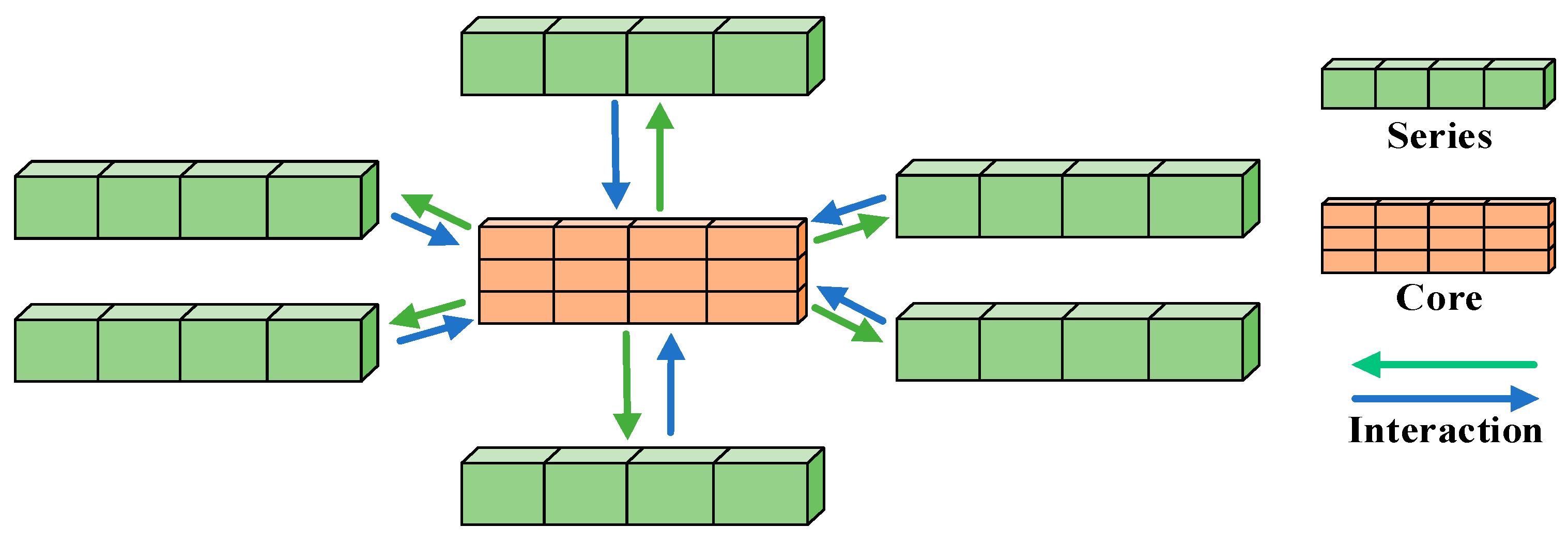
SOFTS is a deep learning architecture built upon the multilayer perceptron (MLP) framework that employs a centralized approach to capture interactions among multiple sequences, achieving state-of-the-art results in multivariate prediction tasks. A key innovation of the SOFTS model is the introduction of the STAR aggregation–redistribution (STAR) module, designed to enhance both the efficiency and accuracy of multivariate time series forecasting [31]. The self-organized mechanism of SOFTS, combined with the STAR random pooling operation, enhances robustness to unusual operating conditions, allowing the model to adapt to input patterns not explicitly observed during training. Figure 1 shows the overall framework of SOFTS, with the specific steps as follows:
(1) Normalize the input multivariate time series, adjusting the series to a state where the mean is zero and the variance is unity, and restore the statistical characteristics prior to normalization after prediction.
(2) Sequence embedding involves linearly projecting the time series data of each channel and embedding it into a d-dimensional vector space.
The input is time series data X ∈ R(C×L), where C is the number of channels and L is the time window length. The output is the sequence embedding representation S0 ∈ R(C×d).
(3) Multilayer STAR modules interact with each other, with each layer of STAR modules responsible for capturing the interrelationships between different channels.
The input is the sequence embedding representation Si−1 from the previous layer. The embedding representation is projected through a multilayer perceptron (MLP) to generate a core representation o∈ Rd, which summarizes the global information of all channels. The core representation o is then concatenated with the sequence embedding representations of each channel to obtain a new fusion representation Fi.
The fused representation is processed using an MLP, and the embedded representation Si is updated via residual connections. The output is the new sequence embedded representation, Si.
(4) Linear projection prediction
After passing through N layers of STAR modules, linear projection is used to convert the final embedded representation SN into the prediction result Ŷ.
The input is the output SN of the STAR module.
The output is the prediction value Ŷ∈ R(C×H), where H is the prediction time step length.
(5) Normalization Restoration: After obtaining the prediction results, the statistical characteristics removed during the normalization process are restored to the prediction values.
STAR Aggregation–Redistribution Module: The STAR module is the core innovation of the SOFTS model [31], designed to efficiently capture dependencies between channels in multivariate time series. The module reduces computational complexity through a centralized structure and improves the model’s robustness to abnormal channels. Although the training data did not cover all possible abnormal oil temperature fluctuations, the design of SOFTS allows the model to generalize to unseen scenarios.
Figure 2 shows the STAR module. The specific working steps of the STAR module are as follows:
Unlike conventional max/average pooling, the STAR module applies a random pooling operation. This introduces controlled stochasticity during feature aggregation, which enhances generalization by preventing the model from overfitting to fixed temporal patterns. It also improves robustness by exposing the model to diverse feature views, similar to an implicit ensemble effect.
(1) Core representation generation: In each layer of the STAR module, a multilayer perceptron (MLP) is first used to generate a global core representation. The core representation reflects the comprehensive information of the multi-channel time series. The calculation formula is as follows:
o = Stoch _ Pool ( MLP 1 ( S i 1 ) )
where S i 1 is the sequence embedding representation from the previous layer, MLP 1 is a mapping function that projects the hidden layer dimension from d to d’, and Stoch _ Pool is a random pooling operation.
(2) Core and sequence fusion: Concatenate the core representation o with the sequence embedding representation S i 1 of each channel to obtain a new representation F i :
F i = Repeat _ Concat ( S i 1 , o )
The operation copies the core representation and connects it to the sequence representation of each channel.
(3) Non-linear transformation: Process the connected representation through another MLP to obtain the updated embedded representation S i :
S i = MLP 2 ( F i ) + S i 1
where MLP 2 is another mapping function that projects the connected representation from d + d’ dimensions back to d dimensions and uses residual connections to enhance the feature representation.

4.2. Hierarchical Bayesian Optimization Algorithm

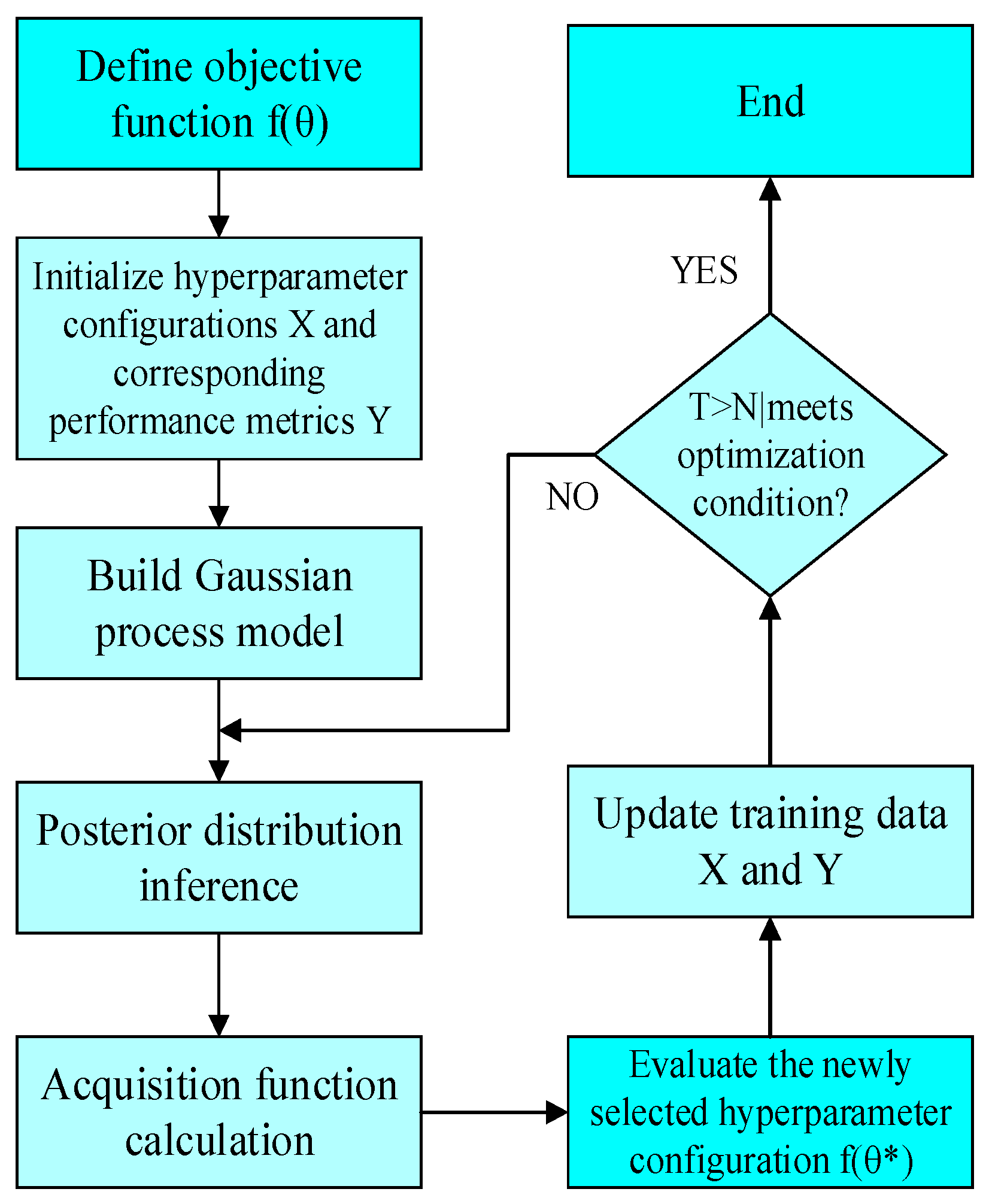
Bayesian optimization is a method that uses probabilistic models to predict the objective function and explores the most valuable optimization methods through function sampling [32]. This paper improves the Gaussian process (GP) optimizer (GP-Tuner) within the Neural Network Intelligence (NNI) framework to enhance model performance and reduce search costs. Hierarchical Bayesian optimization (HBO) divides parameters into control and base layers, reducing coupling and dimensionality issues while improving convergence. In our experiments, HBO converged faster than standard Bayesian optimization and achieved lower final errors. The specific steps are as follows:
(1) Define the parameter space to be optimized. The parameters to be optimized are learning rate (lr), dropout rate (d_ff), training epochs (train_epochs), batch size (batch_size), and model dimension (d_model). The parameter ranges are defined as follows:
θ = [ lr , top _ k , d _ model , d _ ff , dropout , train _ epochs , batch _ size ]
(2) Define the objective function to minimize the mean squared error (MSE) on the validation set. Given the parameter combination, the objective function is
f ( θ ) = 1 N i = 1 N y ^ i y i 2
where y ^ i is the model prediction value, y i is the actual value, and N is the number of samples in the validation set.
Through Bayesian optimization, find the combination of hyperparameters that minimizes f ( θ ) :
θ :   θ = arg min θ   f ( θ )
(3) Initialize the Gaussian process, which is used to model the distribution of the objective function. It constructs an approximate model based on historical observations ( θ , f ( θ ) ) and predicts the performance of new parameter combinations based on this model. The Gaussian process assumes that the values of the objective function follow a multivariate Gaussian distribution:
f ( θ ) G P ( α ( θ ) , k ( θ , θ ) )
where α ( θ ) is the predicted mean, and k ( θ , θ ) is the kernel function (RBF kernel selected), which describes the similarity between parameter combinations.
(4) In Gaussian process optimization, a sampling function is used to determine the parameter combination for the next sampling step. The sampling function used is the upper confidence bound (UCB) sampling function, which takes the following form:
UCB ( θ ) = μ ( θ ) + κ σ ( θ )
where μ ( θ ) represents the current estimated error value, σ ( θ ) represents the predicted uncertainty (variance), and κ represents the mean value predicted by the model for the Gaussian process. The key to optimizing the Gaussian process is to strike a balance between exploring new parameter combinations and utilizing existing optimal parameters through the UCB function.
(5) Iterative update. First, select a parameter combination θ n and calculate its corresponding prediction error f ( θ n ) ; then, update the Gaussian process model with the new observation value ( θ n , f ( θ n ) ) ; next, maximize the acquisition function UCB ( θ ) based on the updated model to find the next set of evaluation parameters θ n + 1 : θ n + 1 = arg max θ UCB ( θ ) ; finally, stop when the maximum number of iterations or convergence criteria is reached.
Introducing the hierarchical Bayesian optimization (HBO) algorithm to improve the efficiency and accuracy of parameter search. Specific steps:
(1) Define the hierarchical parameter space: All model hyperparameters are divided into two levels:
Control layer parameters θ control : Used to control the search space or candidate set of the base layer parameters, specifically including the learning rate range:
θ control = { lr   range = [ 1 e 5 , 1 e 1 ] , batchsize   candidate   set = { 32 , 64 , 128 } , dmodel   candidate   set = { 16 , 32 , 64 } }
Base layer parameters θ base : Under the constraints given by the control layer parameters, the actual parameter combinations used for model training, specifically including
θ base = { l r = 0.0032 , d _ f f = 0.1 , t r a i n _ e p o c h s = 50 , b a t c h _ s i z e = 64 , d _ m o d e l = 32 }
The total parameter space is represented as Θ = { θ control , θ base }
(2) A two-level Bayesian model is adopted. The first level uses GP to model the control parameters and predict the optimal objective function value under this combination. The second level models the underlying parameter space under the control parameters and searches for the optimal underlying layer parameters within the control layer range.
(3) Each round of the optimization process includes the following steps: first, sample θ control ( i ) from the control layer parameter space; then, under the constraints specified by θ control ( i ) , sample θ base ( i ) from the underlying layer parameter space using the GP-UCB strategy to minimize loss; finally, obtain the objective function value f ( θ control ( i ) , θ base ( i ) ) and update the two-layer GP models.
(4) The optimization objective function is expressed as
θ = arg min θ control E θ basc [ f ( θ control , θ base ) ]
That is, search for the combination of control parameters that minimizes the expected loss of the base layer in the control layer space.
Figure 3 illustrates the Gaussian process parameter tuning process, and Table 1 shows the impact of different hyperparameter combinations on the test loss (test_loss) during model training. The impact of different hyperparameter combinations on model performance is not the result of a single parameter but rather the combined effect of multiple parameters. θ* denotes the optimized hyperparameter configuration. For example, a higher learning rate (lr) combined with a smaller model dimension (d_model) may lead to a higher test loss, but if other parameters (such as batch size and training epochs) are appropriately tuned, the loss can still remain low. As shown in Table 1, the first hyperparameter combination (lr = 0.0162674, d_model = 16, d_ff = 8, etc.) achieved the lowest test loss (0.008477), indicating that this combination performs best in the model.

5. Case Study

5.1. Data Source and Preprocessing

This study employs Python 3.11 for simulation analysis, utilizing real operational data from the main transformer of a hydropower station in Yunnan, China, collected hourly between August 2023 and July 2024. A total of 8484 data samples were obtained and subsequently partitioned into training, validation, and test sets with a ratio of 7:1:2. The training data were used to train the SOFTS model, while the test set served for model validation.

5.2. Performance Metrics

Predictions of the transformer top-oil temperature were generated for the test set, and the mean square error (MSE), mean absolute error (MAE), and root mean square error (RMSE) were computed by comparing these predictions with the corresponding actual values. The calculation formulas are presented as follows:
e MSE = 1 N i = 1 N ( Y oil Y ^ oil ) 2 e MAE = 1 N i = 1 N | Y oil Y ^ oil |
e RMSE = 1 N i = 1 N ( Y oil Y ^ oili ) 2
where e MSE is the mean square error, e MAE is the mean absolute error, and e RMSE is the root mean square error.

5.3. Data Processing

Figure 4 shows the five IMFs of the transformer top-oil temperature signal obtained via VMD. The selection of the number of IMFs was further justified by analyzing the relationship between the IMF number and the associated error/residual energy. The optimal number of IMFs, K, was determined by considering both the stability of the center frequencies and the residual information content. When K was less than five, some modes exhibited frequency mixing, whereas for K greater than five, redundant modes appeared, and the reduction in residual energy became marginal.
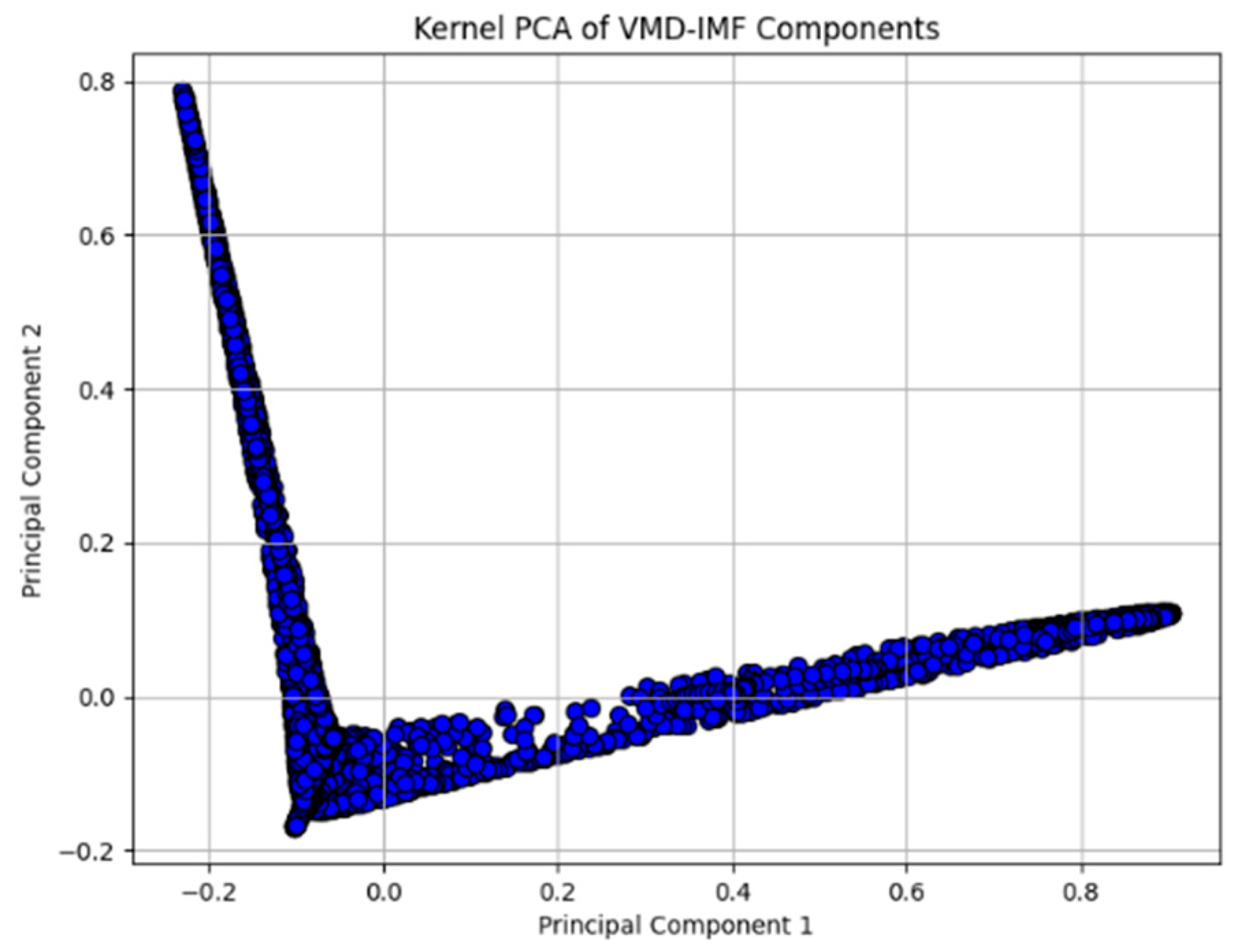
As shown in Table 2, the effect of different IMF numbers on the results, the IMF number was chosen to balance center frequency stability and residual information: fewer than five caused frequency mixing, while more than five introduced redundancy with limited residual energy reduction. VMD decomposes the signal into components across different frequency bands, with IMF 1 capturing the lowest-frequency trend and IMF 5 the highest-frequency fluctuations. Figure 5 presents the Kernel PCA projection of these IMFs onto the first two principal components.
Principal Component 1 and Principal Component 2 are the two dominant components derived from the kernel principal component analysis (KPCA), representing the primary projection directions of the original high-dimensional data in the transformed space. The projection reveals pronounced non-linear characteristics of the data, forming an L-shaped distribution. This pattern suggests that some data points cluster near the origin, while others extend linearly along a specific direction. Such a distribution implies underlying structures within the IMF components, where certain components exhibit high concentration with minimal variation, whereas others display substantial variability. The IMF components obtained via VMD demonstrate complex non-linear relationships, which KPCA effectively captures and visualizes in a reduced-dimensional space. This visualization is crucial for further analysis of the features and interrelations among the IMF components.
VMD was adopted as it adaptively determines mode frequency and bandwidth to mitigate mixing and boundary effects, allows predefined IMF numbers for stable decomposition, and produces more stationary IMFs that support Kernel PCA and TSHAP-MLP-based feature analysis.

5.4. Multivariate Input Feature Selection

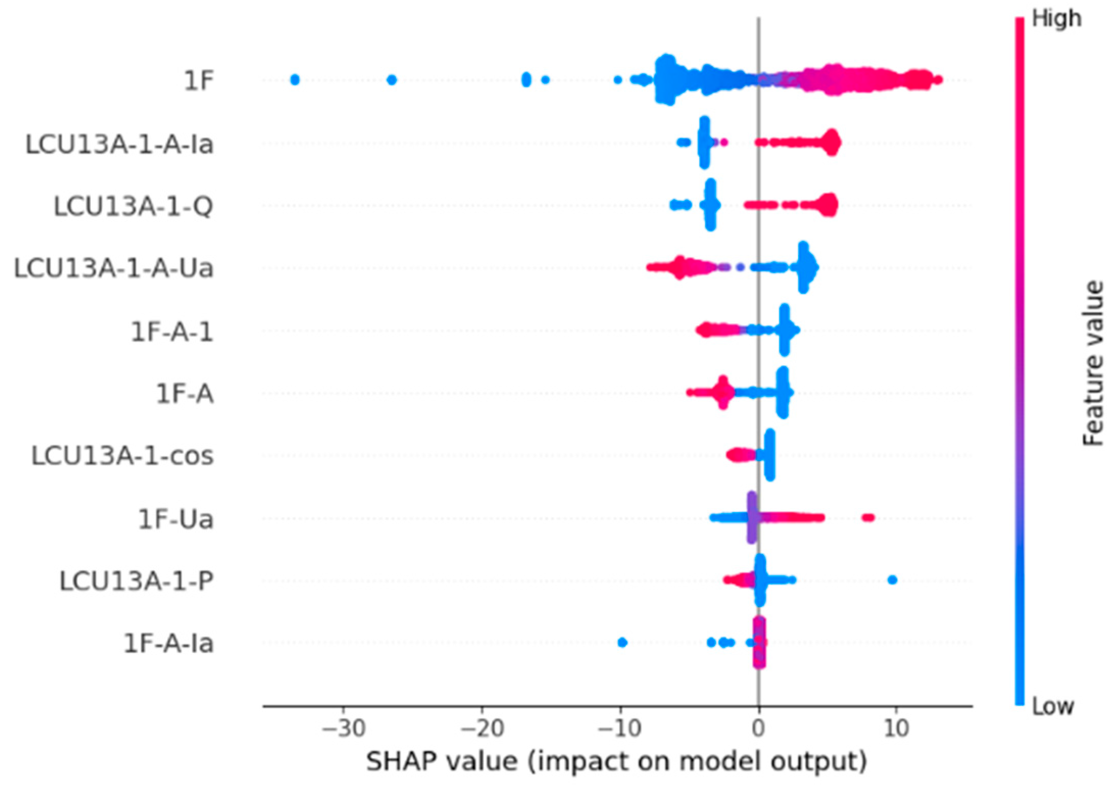
Table 3 lists the SHAP values for each feature, and Figure 6 shows the relationship between different features and the model output, where the X-axis represents the SHAP value of the feature. The larger the SHAP value, the greater the influence of the feature on the output result, and vice versa. Positive values indicate that the feature increases the predicted value, while negative values indicate that it decreases the predicted value. The Y-axis includes the abbreviations for each feature, and the color of the points represents the feature’s value, ranging from blue (low value) to red (high value), i.e., the feature’s value range. The redder the color, the higher the feature’s value, while blue indicates a lower value. The horizontal distribution shows how the SHAP values of each feature are distributed across different samples. The more scattered the points, the greater the variation in the feature’s impact on different samples. For example, the 1F feature (main variable A winding temperature) has a significant impact, with SHAP values ranging from −30 to 10 and red and blue points interspersed, indicating that the feature has a substantial positive or negative impact on the model output across different samples. It is worth noting that some features exhibit both positive and negative SHAP contributions with a wide spread. This reflects their bidirectional physical role in transformer thermal behavior: for instance, ambient temperature and load variations may exert opposite influences under different cooling or seasonal conditions. Such wide distributions highlight context-dependent dynamics rather than model instability. The wide SHAP value distributions observed for certain features indicate that their influence on transformer top-oil temperature is not unidirectional but varies with operating context. This aligns with physical understanding, where the same factor may act differently under varying load and cooling conditions.
Based on the SHAP values in Figure 6 and Table 3, the larger the SHAP value, the greater the influence of that feature on the model’s prediction. Remove features with SHAP values less than 1 and select other features with high importance as model inputs. Table 4 (effect of SHAP threshold on results) summarizes the influence of different thresholds. A threshold of |SHAP| > 1 was adopted for feature retention in this study. This value was determined by comparing predictive performance under different thresholds. When the threshold is too low (e.g., 0.2), many redundant features are retained, potentially leading to overfitting; when it is too high (e.g., 4), some critical features are discarded, resulting in insufficient information for the model.

6. Results Comparison

6.1. Analysis of Transformer Top Oil Temperature Prediction Results Based on SOFTS

A SOFTS training program was developed using Python to train the 5918 samples in the training set, validate the 850 samples in the validation set, and test the 1696 samples in the test set. While dedicated noise experiments were not performed, the integrated framework of VMD decomposition, SHAP-guided feature selection, and SOFTS adaptation, complemented by standard preprocessing of outliers and missing data, inherently enhances the model’s robustness to noise and incomplete sensor measurements.
Figure 7 illustrates the comparison between the actual top-oil temperature of the transformer and the corresponding predictions generated by the SOFTS model. The blue line reflects the true temperature trend, characterized by periodic fluctuations, while the orange dotted line represents the SOFTS model’s predicted values. Overall, the model’s predictions exhibit strong agreement with the actual data, particularly in the later phase (right side of the figure), where it accurately captures the steady upward trend and subtle temperature variations.
As time progresses, the SOFTS model gradually demonstrates its advantage in capturing long-term and short-term dependencies, particularly excelling in the more stable fluctuations in the later stages, where the predicted results closely align with the actual values. Unlike earlier hybrid frameworks that mainly combine signal decomposition with traditional neural models, our method uniquely integrates VMD, Kernel PCA, and time-aware SHAP with a self-organized forecasting backbone optimized by hierarchical Bayesian search. This synergy enables both higher accuracy and greater adaptability under varying operating conditions.
Table 5 presents the RMSE results obtained from the SOFTS model’s prediction of the transformer’s top-layer oil temperature, representing the standard deviation between predicted and actual values. The RMSE is 0.632, indicating a low level of prediction error. The MAE, which measures the average absolute error between predicted and actual values, is 0.396, suggesting that the average deviation per prediction point is relatively small. This low MAE further confirms the model’s strong predictive capability, with consistently minimal errors in forecasting top-oil temperature.
To demonstrate the advantages of the model proposed in this experiment from multiple perspectives, Table 5 also presents the coefficient of determination (R2), symmetric mean absolute percentage error (sMAPE), and Nash–Sutcliffe efficiency coefficient (NSE) of the experimental results obtained using the model. R2 reflects the model’s explanatory power, with a value of 0.982, indicating that 98.2% of the fluctuations in top-layer oil temperature can be well explained by the model. sMAPE is a symmetric percentage error metric that considers the relative difference between predicted and actual values. The closer the value is to 0, the smaller the relative error of the model. Here, sMAPE is 0.0107, meaning that the model’s prediction error accounts for only 1.07% of the actual value. NSE is used to evaluate the accuracy of model predictions, with a higher value indicating better predictive performance. Here, NSE is 0.982, indicating that the model’s predictive accuracy is very high, approaching perfect prediction. The comprehensive performance of these indicators shows that the SOFTS model can effectively perform accurate predictions of transformer top-oil temperature and that the model has high robustness and stability.

6.2. Comparison of SOFTS Parameter Tuning Results

Figure 8 presents a comparison of the SOFTS model’s prediction performance before and after parameter tuning for transformer top-oil temperature. The blue line denotes the actual top-oil temperature, while the orange line illustrates the predicted values generated by the SOFTS model prior to parameter optimization. Although the orange curve generally follows the trend of the actual values, it exhibits considerable discrepancies in fluctuation amplitude at several points, particularly in regions characterized by rapid temperature changes, where it fails to accurately capture peak values. In contrast, the red line reflects the prediction outcomes after parameter tuning. Compared to the orange line, it can be observed that the red line shows a significant improvement in agreement with the actual values after parameter tuning. After parameter tuning, the model’s prediction accuracy has significantly improved, especially during the initial phase of intense fluctuations, where the model can better fit the actual data. This indicates that by adjusting parameters such as the learning rate, feature dimension, and regularization parameters, the model’s ability to capture temperature time-series fluctuations can be effectively enhanced.

6.3. Comparative Analysis of Different Deep Learning Models

To evaluate the performance of the SOFTS model in forecasting transformer top-oil temperature, this study compares it with several deep learning approaches, including transformer [33], TimesNet [34], LSTM [35], and the traditional BP algorithm [36]. The same test samples as described in Section 3.1 are utilized. For the transformer and TimesNet models, the dataset is split into training, validation, and test sets in a ratio of 7:1:2. In contrast, for LSTM and BP, the data are divided into training and test sets using an 8:2 split.
LSTM and BP follow their original 8:2 training–test split, whereas transformer, TimesNet, and SOFTS-NNI use a 7:1:2 chronological split. All models share an identical, temporally non-overlapping test set. The validation portion available to transformer, TimesNet, and SOFTS-NNI (10% of the data) is employed for early stopping and hyperparameter tuning, ensuring that every architecture leverages the same total amount of data for learning while being evaluated on the same strictly held-out samples. And to ensure fairness, all baseline models were tuned using standard Bayesian optimization, with the search space covering key hyperparameters such as network depth, number of hidden units, learning rate, and dropout ratio, with a maximum of 100 iterations. The SOFTS model was further refined using the proposed hierarchical Bayesian optimization for more precise tuning. The computational evaluation shows that the training phase required less than 60 s and the inference phase less than 5 s, indicating that the overall computational burden remains low and fully meets the requirements of real-time monitoring applications.
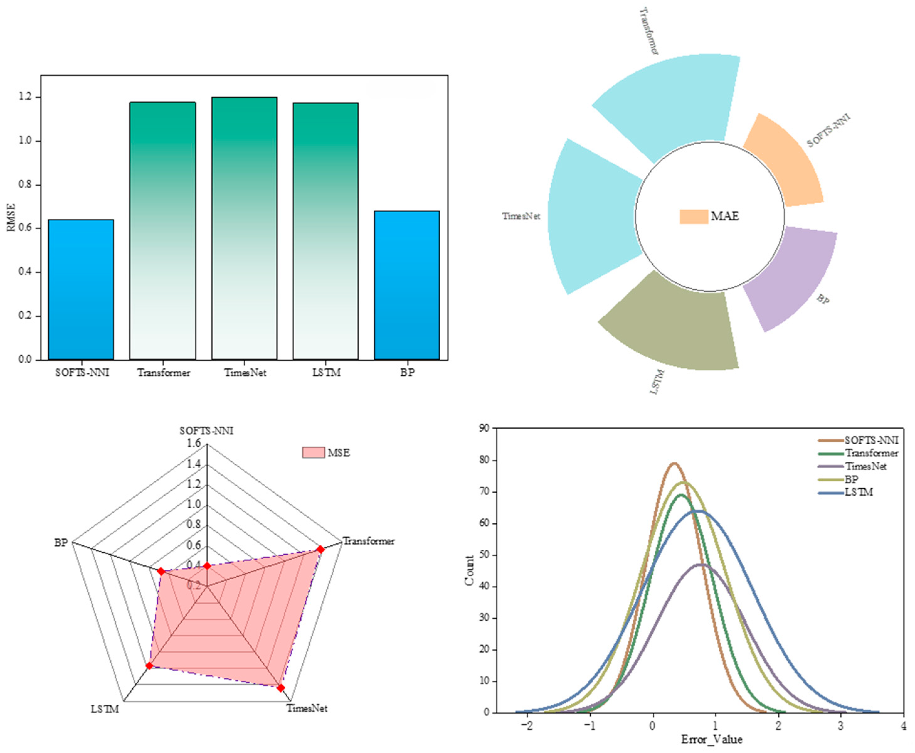
Figure 9 compares the top-oil temperature prediction results of the transformer using five different machine learning models. As shown in Figure 10, an analysis of the prediction errors reveals that the SOFTS model demonstrates strong consistency with actual temperature fluctuations, especially during the mid-term period characterized by frequent peaks and troughs, where it accurately captures the dynamic variations in the data. It is observed that transformer shows clustered error spikes, which stem from its reliance on historical attention when facing regime shifts. In contrast, SOFTS-NNI produces smoother error distributions due to multi-scale decomposition and adaptive pooling. In contrast, both the transformer and TimesNet models show delayed responses to changes, particularly at extreme points, leading to noticeable deviations from the actual values and an inability to effectively capture fluctuation patterns. The LSTM model exhibits substantial prediction errors during the early and mid-term stages, reflecting poor responsiveness to sudden changes; although its performance improves in the later stage, it still lags behind the other models. Notably, during periods of rapid top-oil temperature variation, the SOFTS model responds more promptly, whereas the BP model displays a delayed reaction in certain instances.
The error sensitivity of different models to sudden input variations reflects their architectural characteristics. While BP and LSTM tend to show abrupt error spikes, transformer-based models may cluster errors when historical contexts differ from the current regime. In contrast, SOFTS combines decomposition, feature selection, and adaptive pooling to alleviate this sensitivity, leading to smoother error distributions under sudden changes. The clustered high errors in the transformer reflect the intrinsic sensitivity of attention-based models to abrupt regime changes. By contrast, SOFTS-NNI integrates decomposition, feature selection, and adaptive pooling, which smooths error distribution and enhances robustness under dynamic conditions. The BP model performs relatively well under stable load conditions due to the monotonicity and regularity of top-oil temperature data, allowing shallow networks to capture the load–temperature mapping. However, BP errors may increase significantly under abrupt fluctuations and seasonal changes, indicating a possible lack of robustness. In contrast, SOFTS demonstrates superior stability and generalization under complex conditions, highlighting the benefits of deep architectures and dynamic feature modeling.
Overall, the computational analysis demonstrates that despite the integration of additional modules, efficiency is well preserved, with preprocessing contributing minimally, SOFTS forward propagation remaining the main cost, and only marginal overhead observed in both training and real-time inference.
Table 6 shows the evaluation indicators obtained by the five different models when performing top-layer oil temperature calculations, and Figure 11 shows the evaluation indicator analysis chart corresponding to the five different models.
Based on the results presented in Table 6 and Figure 11, the SOFTS-NNI model—optimized using the Bayesian optimization algorithm—achieves strong performance across all three evaluation metrics, particularly exhibiting notably low RMSE and MSE values. Compared with the best-performing alternative (the BP model), SOFTS-NNI achieves reductions of 18.71% in RMSE, 27.75% in MSE, and 14.31% in MAE, indicating a significant improvement in predictive accuracy. The relatively low MAE further reflects the model’s ability to minimize average prediction errors. Overall, the SOFTS model demonstrates outstanding performance across all evaluation indicators, achieving the lowest values of RMSE, MSE, and MAE, thereby confirming its superiority in forecasting transformer top-oil temperature. Although this study is based on a single operational dataset, the observed error distribution patterns primarily reflect the intrinsic modeling capabilities of the different architectures. Therefore, while absolute errors may vary across other datasets, the relative trends in error distribution are expected to remain consistent. Although no dedicated experiments on seasonal or abrupt changes were conducted, the framework is inherently designed to handle such scenarios. VMD decomposes the signal into IMFs capturing long-term seasonal trends and short-term fluctuations, TSHAP dynamically adjusts the relative importance of seasonal and load-dependent features, and the SOFTS STAR module enhances adaptability via stochastic pooling. Collectively, these mechanisms improve the framework’s robustness against both seasonal variations and abrupt load changes.

7. Conclusions

To address the issues of low accuracy and weak interference resistance in transformer oil temperature prediction, this paper proposes a transformer oil temperature prediction method that combines VMD, Kernel PCA, SHAP-MLP feature selection methods, and the SOFTS deep learning model. Using historical oil temperature data from the main transformer of a hydropower station in Yunnan, China, as a case study, this paper conducts experimental research and draws the following conclusions:
(1)
When compared with traditional neural network models such as BP and other deep learning models like LSTM, transformer, and TimesNet, the SOFTS model demonstrated significant advantages in terms of prediction accuracy and model stability. Experimental results show that the SOFTS model, optimized using Bayesian optimization algorithms, achieved the smallest evaluation metrics (RMSE, MSE, and MAE) in top-level oil temperature prediction, indicating higher prediction accuracy and lower error rates.
(2)
This study combines VMD and Kernel PCA methods for feature extraction of top-level oil temperature signals and uses the SHAP-MLP feature selection method to optimize input features, significantly improving the model’s prediction accuracy. The combination of these techniques effectively reduces the model’s input dimension, removes redundant features, and enhances the model’s generalization capability and efficiency.
(3)
This study provides an effective deep learning method for transformer top-layer oil temperature prediction, demonstrating its practical application value in power equipment monitoring. Future research will continue to explore other optimization algorithms and model structures to further enhance the prediction performance of transformer operating conditions, particularly in terms of stability and robustness in complex environments.
(4)
This study demonstrates the effectiveness of the SOFTS framework on hydropower transformer data. Leveraging the universal thermal–electrical load coupling, VMD and KPCA extract transferable features, TSHAP-MLP identifies key variables across operating conditions, and the STAR module adapts to diverse load patterns. Future work will validate the method on transformers with varying capacities, cooling methods, and regional grid conditions and explore transfer learning to enhance cross-device generalization.
(5)
The distinctiveness of this study lies in the multi-level integration of decomposition, non-linear reduction, temporal feature selection, and adaptive forecasting, which has not been explored in previous transformer temperature prediction works. Future work will explicitly evaluate the proposed framework under noisy and incomplete data, which are common in real-world monitoring systems, and will extend validation to datasets exhibiting stronger seasonal cycles and more frequent abrupt load fluctuations, thereby providing a more quantitative assessment of its adaptability.
(6)
Beyond methodological improvements, advances in transformer insulating liquids are also reshaping the thermal environment of power equipment. Khelifa et al. [37] showed that adding ZrO2 nanoparticles to mineral, synthetic, and natural esters can significantly enhance AC breakdown voltage at optimal concentrations, improving insulation reliability. Koutras et al. [38] further reported that semiconducting nanoparticles (SiC, TiO2) improve the initial thermal and dielectric performance of natural esters but may accelerate agglomeration and property degradation with aging. These findings highlight that material-driven changes affect heat dissipation and insulation stability, underscoring the need for accurate top-oil temperature forecasting in next-generation transformers.

Author Contributions

Z.T.: conceptualization, data curation, and methodology; Y.X.: writing—review and editing; X.M.: software and visualization; Y.Z.: methodology, investigation, software, and writing—original draft; T.P.: conceptualization and methodology; C.Z.: conceptualization and writing—review and editing. All authors have read and agreed to the published version of the manuscript.

Funding

This work is supported by China Yangtze Power Co., Ltd. (CYPC) Sponsored Project (Z522302017).

Data Availability Statement

The data presented in this study are available on request from the corresponding author.

Conflicts of Interest

Authors Zhixiang Tong and Yan Xu were employed by the company China Yangtze Power Co., Ltd. Authors Xianyu Meng, Yongshun Zheng, Tian Peng and Chu Zhang were employed by the company NARI Engineering Technology Co., Ltd.

Abbreviations

VMDVariational Mode Decomposition
BiGRUBidirectional Gated Recurrent Unit
Kernel PCAKernel Principal Component Analysis
BWOBlack Widow Optimization
ELMExtreme Learning Machines
IMFIntrinsic Mode Function
SVMSupport Vector Machines
MLPMultilayer Perceptron
RMSERoot Mean Square Error
CNNConvolutional Neural Network
BiLSTMBidirectional Long Short-Term Memory
LSTMLong Short-Term Memory
RNNRecurrent Neural Network
CEEMDANComplete Ensemble Empirical Mode Decomposition with Adaptive Noise
SASelf-Attention
EEMDEnsemble Empirical Mode Decomposition
PSOParticle Swarm Optimization
TOTTop Oil Temperature
HKELMHybrid Kernel Extreme Learning Machine
IWOAImproved Whale Optimization Algorithm
TCNTemporal Convolutional Network
SOFTSSelf-organized Time Series Forecasting System
NSENash–Sutcliffe Efficiency
MAERoot Mean Absolute Error
sMAPESymmetric Mean Absolute Percentage Error
EMDEmpirical Mode Decomposition
R2Coefficient of Determination
MSEMean Squared Error
KELMKernel Extreme Learning Machine

References

  1. Li, S.; Xue, J.; Wu, M.; Xie, R.; Jin, B.; Wang, K. Prediction of transformer top oil temperature based on improved weighted support vector regression based on particle swarm optimization. In Proceedings of the 2021 International Conference on Advanced Electrical Equipment and Reliable Operation (AEERO), Beijing, China, 15–17 October 2021; IEEE: Piscataway, NJ, USA, 2021; pp. 1–5. [Google Scholar]
  2. Huang, X.; Zhuang, X.; Tian, F.; Niu, Z.; Chen, Y.; Zhou, Q.; Yuan, C. A Hybrid ARIMA-LSTM-XGBoost Model with Linear Regression Stacking for Transformer Oil Temperature Prediction. Energies 2025, 18, 1432. [Google Scholar] [CrossRef]
  3. Zhang, C.; Ma, H.; Hua, L.; Sun, W.; Nazir, M.S.; Peng, T. An evolutionary deep learning model based on TVFEMD, improved sine cosine algorithm, CNN and BiLSTM for wind speed prediction. Energy 2022, 254, 124250. [Google Scholar] [CrossRef]
  4. Peng, T.; Zhang, C.; Zhou, J.; Nazir, M.S. An integrated framework of Bi-directional long-short term memory (BiLSTM) based on sine cosine algorithm for hourly solar radiation forecasting. Energy 2021, 221, 119887. [Google Scholar] [CrossRef]
  5. Guo, Y.; Chang, Y.; Lu, B. A review of temperature prediction methods for oil-immersed transformers. Measurement 2025, 239, 115383. [Google Scholar] [CrossRef]
  6. Dong, N.; Zhang, R.; Li, Z.; Cao, B. Prediction model of transformer top oil temperature based on data quality enhancement. Rev. Sci. Instrum. 2023, 94, 074707. [Google Scholar] [CrossRef] [PubMed]
  7. Deng, W.; Yang, J.; Liu, Y.; Wu, C.; Zhao, Y.; Liu, X.; You, J. A Novel EEMD-LSTM Combined Model for Transformer Top-Oil Temperature Prediction. In Proceedings of the 2021 8th International Forum on Electrical Engineering and Automation (IFEEA), Xi’an, China, 3–5 September 2021; IEEE: Piscataway, NJ, USA, 2021; pp. 52–56. [Google Scholar]
  8. Cao, Y. An Improved Prediction Method of Transformer Oil Temperature. In Proceedings of the 2023 IEEE 6th Information Technology, Networking, Electronic and Automation Control Conference (ITNEC), Chongqing, China, 24–26 February 2023; IEEE: Piscataway, NJ, USA, 2023; pp. 987–991. [Google Scholar]
  9. Hu, J.; Liu, Y.; Peng, Y.; Chen, C.; Wan, J.; Cao, B. Data-Driven short-term prediction for top oil temperature of Residential Transformer. In Proceedings of the 2022 China International Conference on Electricity Distribution (CICED), Changsha, China, 7–8 September 2022; IEEE: Piscataway, NJ, USA, 2022; pp. 303–309. [Google Scholar]
  10. Chang, J.; Duan, X.; Tao, J.; Ma, C.; Liao, M. Power Transformer Oil Temperature Prediction Based on Spark Deep Learning. In Proceedings of the 2022 IEEE International Conference on High Voltage Engineering and Applications (ICHVE), Chongqing, China, 25–29 September 2022; IEEE: Piscataway, NJ, USA, 2022; pp. 1–4. [Google Scholar]
  11. Wang, K.; Zhang, H.; Wang, X.; Li, Q. Prediction method of transformer top oil temperature based on VMD and GRU neural network. In Proceedings of the 2020 IEEE International Conference on High Voltage Engineering and Application (ICHVE), Beijing, China, 6–10 September 2020; IEEE: Piscataway, NJ, USA, 2020; pp. 1–4. [Google Scholar]
  12. Wang, X.; Fu, C.; Zhao, Z.; Fu, B.; Jiang, T.; Xu, Y.; Zhang, L.; Hou, Y. Prediction of transformer top oil temperature based on AC-BiLSTM model. In Proceedings of the 2023 4th International Conference on Smart Grid and Energy Engineering (SGEE), Zhengzhou, China, 24–26 November 2023; IEEE: Piscataway, NJ, USA, 2023; pp. 390–394. [Google Scholar]
  13. Lei, L.; Liao, F.; Liu, B.; Tang, P.; Zheng, Z.; Qi, Z.; Zhang, Z. Research on Transformer Temperature Rise Prediction and Fault Warning Based on Attention-GRU. In Proceedings of the 2023 5th International Conference on Smart Power & Internet Energy Systems (SPIES), Shenyang, China, 1–4 December 2023; IEEE: Piscataway, NJ, USA, 2023; pp. 94–99. [Google Scholar]
  14. Wang, Y.Q.; Yue, G.L.; He, J.; Liu, H.L.; Bi, J.G.; Chen, S.F. Research on Top-Oil Temperature Prediction of Power Transformer Based on Kalman Filtering Algorithm. High Volt. Appar. 2014, 50, 74–79+86. [Google Scholar]
  15. Dong, X.; Jing, L.; Tian, R.; Dong, X. Transformer Top-Oil Temperature Prediction Method Based on LSTM Model. Proc. China Electr. Power Soc. 2023, 38, 38–45. [Google Scholar]
  16. Yang, J.; Lu, W.; Liu, X. Prediction of Top Oil Temperature for Oil-immersed Transformers Based on PSO-LSTM. In Proceedings of the 2021 4th International Conference on Energy, Electrical and Power Engineering (CEEPE), Chongqing, China, 23–25 April 2021; IEEE: Piscataway, NJ, USA, 2021; pp. 278–283. [Google Scholar]
  17. Zou, D.; Xu, H.; Quan, H.; Yin, J.; Peng, Q.; Wang, S.; Dai, W.; Hong, Z. Top-Oil Temperature Prediction of Power Transformer Based on Long Short-Term Memory Neural Network with Self-Attention Mechanism Optimized by Improved Whale Optimization Algorithm. Symmetry 2024, 16, 1382. [Google Scholar] [CrossRef]
  18. Liu, J.; Hou, Z.; Liu, B.; Zhou, X. Mathematical and Machine Learning Innovations for Power Systems: Predicting Transformer Oil Temperature with Beluga Whale Optimization-Based Hybrid Neural Networks. Mathematics 2025, 13, 1785. [Google Scholar] [CrossRef]
  19. Hao, Y.; Zhang, Z.; Liu, X.; Yang, Y.; Liu, J. Inversion Method for Transformer Winding Hot Spot Temperature Based on Gated Recurrent Unit and Self-Attention and Temperature Lag. Sensors 2024, 24, 4734. [Google Scholar] [CrossRef]
  20. Zhang, Z.; Kong, W.; Li, L.; Zhao, H.; Xin, C. Prediction of transformer oil temperature based on an improved pso neural network algorithm. In Recent Advances in Electrical & Electronic Engineering (Formerly Recent Patents on Electrical & Electronic Engineering); Bentham Science Publishers: Sharjah, United Arab Emirates, 2024; Volume 17, pp. 29–37. [Google Scholar]
  21. Li, K.; Xu, Y.; Wei, B.; Hua, H.; Qi, X. Transformer Top-Oil Temperature Prediction Model Based on PSO-HKELM. High Volt. Eng. 2018, 44, 2501–2508. [Google Scholar]
  22. Li, R. Research on Transformer Top-Oil Temperature Prediction Method Based on Bayesian Network. Master’s Thesis, Southwest Jiaotong University, Chengdu, China, 2018. [Google Scholar]
  23. Qi, X.; Li, K.; Yu, X.; Lou, J. Transformer Top-Oil Temperature Interval Prediction Based on Kernel Extreme Learning Machine and Bootstrap Method. Proc. Chin. Soc. Electr. Eng. 2017, 37, 5821–5828+5860. [Google Scholar]
  24. Li, S.; Xue, J.; Wu, M.; Xie, R.; Jin, B.; Zhang, H.; Li, Q. Transformer Top-Oil Temperature Prediction Based on Particle Swarm Optimization Improved Weighted Support Vector Regression. High Volt. Appar. 2021, 5, 103–109. [Google Scholar]
  25. Patro, S.; Sahu, K.K. Normalization: A preprocessing stage. arXiv 2015, arXiv:1503.06462. [Google Scholar] [CrossRef]
  26. Dragomiretskiy, K.; Zosso, D. Variational Mode Decomposition. IEEE Trans. Signal Process. 2014, 62, 531–544. [Google Scholar] [CrossRef]
  27. Zhang, C.; Li, Z.; Ge, Y.; Liu, Q.; Suo, L.; Song, S.; Peng, T. Enhancing short-term wind speed prediction based on an outlier-robust ensemble deep random vector functional link network with AOA-optimized VMD. Energy 2024, 296, 131173. [Google Scholar] [CrossRef]
  28. Schölkopf, B.; Smola, A.; Müller, K.-R. Kernel principal component analysis. In Artificial Neural Networks—ICANN’97; Gerstner, W., Germond, A., Hasler, M., Nicoud, J.-D., Eds.; Springer: Berlin/Heidelberg, Germany, 1997; Volume 1327, pp. 583–588. [Google Scholar]
  29. Lundberg, S.M.; Lee, S.-I. A unified approach to interpreting model predictions. In Proceedings of the 31st International Conference on Neural Information Processing Systems (NeurIPS 2017), Long Beach, CA, USA, 4–9 December 2017; Curran Associates, Inc.: Red Hook, NY, USA, 2017; Volume 30. [Google Scholar]
  30. Taud, H.; Mas, J.F. Multilayer Perceptron (MLP). In Geomatic Approaches for Modeling Land Change Scenarios; Camacho Olmedo, M.T., Paegelow, M., Mas, J.-F., Escobar, F., Eds.; Springer International Publishing: Cham, Switzerland, 2018; pp. 451–455. [Google Scholar]
  31. Han, L.; Chen, X.-Y.; Ye, H.-J.; Zhan, D.-C. Softs: Efficient multivariate time series forecasting with series-core fusion. arXiv 2024, arXiv:2404.14197. [Google Scholar] [CrossRef]
  32. Snoek, J.; Larochelle, H.; Adams, R.P. Practical Bayesian optimization of machine learning algorithms. In Proceedings of the 25th International Conference on Neural Information Processing Systems (NeurIPS 2012), Lake Tahoe, NV, USA, 3–6 December 2012; Curran Associates, Inc.: Red Hook, NY, USA, 2012; Volume 25. [Google Scholar]
  33. Vaswani, A.; Shazeer, N.; Parmar, N.; Uszkoreit, J.; Jones, L.; Gomez, A.N.; Kaiser, Ł.; Polosukhin, I. Attention is all you need. In Proceedings of the 31st International Conference on Neural Information Processing Systems (NeurIPS 2017), Long Beach, CA, USA, 4–9 December 2017; Curran Associates, Inc.: Red Hook, NY, USA, 2017; Volume 30. [Google Scholar]
  34. Wu, H.; Hu, T.; Liu, Y.; Zhou, H.; Wang, J.; Long, M. Timesnet: Temporal 2d-variation modeling for general time series analysis. arXiv 2022, arXiv:2210.02186. [Google Scholar]
  35. Hochreiter, S.; Schmidhuber, J. Long Short-Term Memory. Neural Comput. 1997, 9, 1735–1780. [Google Scholar] [CrossRef]
  36. Rumelhart, D.E.; Hinton, G.E.; Williams, R.J. Learning representations by back-propagating errors. Nature 1986, 323, 533–536. [Google Scholar] [CrossRef]
  37. Khelifa, H.; Vagnon, E.; Beroual, A. Effect of zirconia nanoparticles on the AC breakdown voltage of mineral oil, synthetic, and natural esters. IEEE Trans. Dielectr. Electr. Insul. 2024, 31, 731–737. [Google Scholar] [CrossRef]
  38. Koutras, K.N.; Peppas, G.D.; Tegopoulos, S.N.; Kyritsis, A.; Yiotis, A.G.; Tsovilis, T.E.; Gonos, I.F.; Pyrgioti, E.C. Aging impact on relative permittivity, thermal properties, and lightning impulse voltage performance of natural ester oil filled with semiconducting nanoparticles. IEEE Trans. Dielectr. Electr. Insul. 2023, 30, 1598–1607. [Google Scholar] [CrossRef]
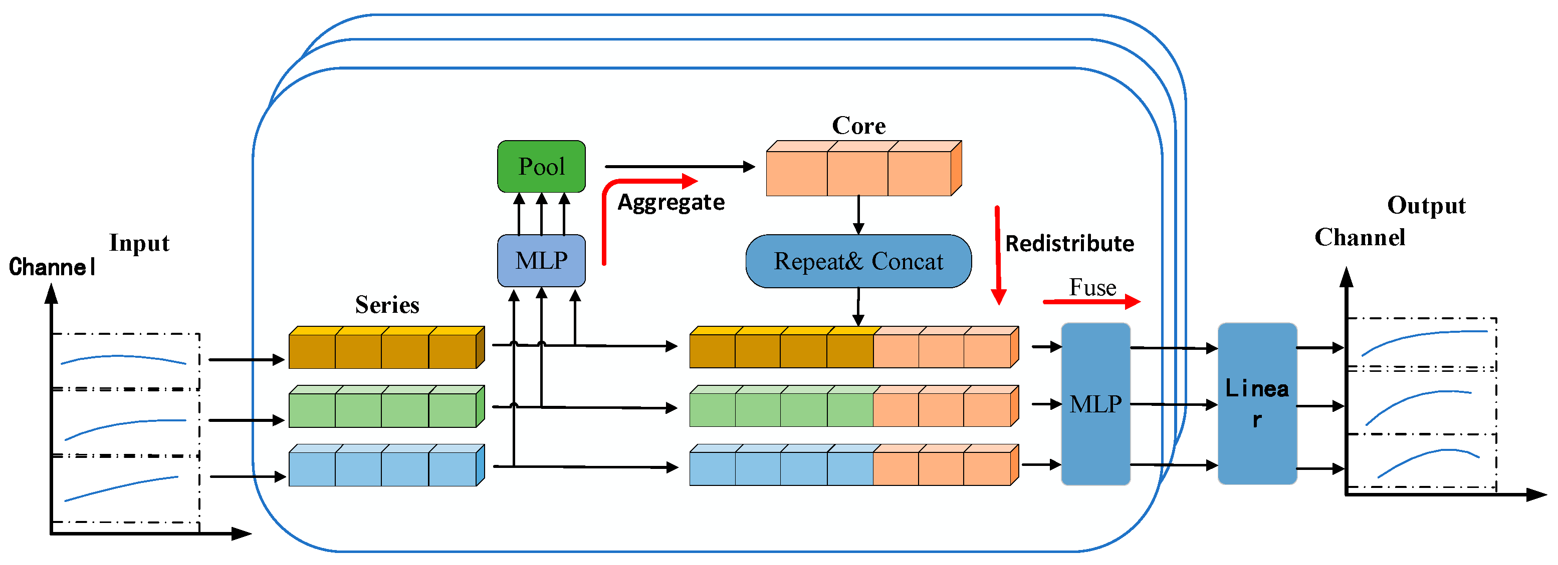
Figure 1. The overall framework diagram of SOFTS [31].
Processes 13 02888 g001
Figure 2. The structure of the STAR module [31].
Processes 13 02888 g002
Figure 3. Parameter optimization process using the Bayesian algorithm.
Processes 13 02888 g003
Figure 4. VMD_IMF decomposition results.
Processes 13 02888 g004
Figure 5. Kernel PCA components of VMD-IMFs.
Processes 13 02888 g005
Figure 6. SHAP value impact analysis diagram.
Processes 13 02888 g006
Figure 7. Comparison of SOFTS predicted values and ground truth.
Processes 13 02888 g007
Figure 8. SOFTS model prediction comparison with and without parameter optimization.
Processes 13 02888 g008
Figure 9. Comparison of temperature prediction results from different models.
Processes 13 02888 g009
Figure 10. Comparison of error values across different models.
Processes 13 02888 g010
Figure 11. Visualization of evaluation metrics for various models.
Processes 13 02888 g011
Table 1. Selected parameters and errors from Bayesian optimization (partial).
Parameters of the SOFTS Deep Learning Model
lrd_modeld_ffdropoutTrain_EpochsBatch_SizeTest_Loss
0.016271680.0619416890.008477
0.08974880.1219417900.024948
0.000133280.1219415900.036025
0.000148160.001958880.096082
0.0863532320.07821161120.164758
Table 2. The effect of different IMF numbers on the results.
Number of IMFs K Residual Energy (%)RMSEMAE
312.40.720.57
47.10.650.52
54.80.630.50
64.60.650.51
74.50.660.52
84.50.670.53
Table 3. SHAP values of individual features.
AbbreviationFeature DescriptionSHAP Value
1F1F: Main transformer phase A winding temperature6.158109
LCU13A-1-A-IaLCU13A: No. 1 main transformer HV side power factor cos4.533494
LCU13A-1-Q1F: Outlet A phase voltage Ua4.246660
LCU13A-1-A-UaLCU13A: Active power on the high-voltage side
of No. 1 main transformer
4.204933
1F-A-11F: Active power (transmitter 1)2.454016
1F-ALCU13A: No. 1 main transformer HV side phase A current Ia2.163187
LCU13A-1-cos1F: Outlet A phase current Ia1.013335
1F-UaLCU13A: No. 1 main transformer high-voltage side reactive power Q0.874439
LCU13A-1-P1F: Reactive power0.454664
1F-A-IaLCU13A: No. 1 main transformer HV side power factor cos0.206889
Table 4. Effect of SHAP threshold on results.
SHAP ThresholdNumber of Retained FeaturesRMSEMAE
0.2100.690.56
1.070.630.50
440.660.53
Table 5. Data of evaluation metrics.
Error_NameSOFTS_Error_Value
RMSE0.63221
MAE0.39568
R20.98195
MSE0.39969
SMAPE0.01069
NSE0.98204
Table 6. Performance evaluation metrics for various models.
Models e RMSE e MSE e MAE
SOFTS-NNI0.63580.39970.3990
Transformer1.17331.37680.9009
TimesNet1.19861.43670.8975
LSTM1.08061.16790.8089
BP0.82290.67720.5422
Disclaimer/Publisher’s Note: The statements, opinions and data contained in all publications are solely those of the individual author(s) and contributor(s) and not of MDPI and/or the editor(s). MDPI and/or the editor(s) disclaim responsibility for any injury to people or property resulting from any ideas, methods, instructions or products referred to in the content.