Numerical Simulation Study of Gas Leakage and Diffusion in Underground Comprehensive Pipe Gallery

Abstract

To reveal the dispersion characteristics of gas leaks in a comprehensive pipe gallery under different leakage parameters, a refined model for gas leak dispersion was established based on CFD simulation. By studying parameters such as alarm time, methane diffusion distance, and backflow length, the impact of leakage aperture and pipeline operating pressure on the distribution characteristics of gas leaks in the comprehensive pipe gallery was investigated. Furthermore, prediction models for alarm time, methane diffusion distance, and backflow length were developed. The results show the following: (a) When the pipeline operating pressure is constant, the leakage rate increases according to a power-law relationship with the size of the leakage aperture. However, when the leakage aperture size is constant, the leakage rate exhibits a linear relationship with the pipeline operating pressure; (b) The alarm time decreases with an increase in both the leakage aperture and pipeline operating pressure. Similarly, the methane diffusion distance increases with an increase in these two factors. Moreover, the methane backflow length increases according to a power-law relationship with the dimensionless leakage aperture and pipeline operating pressure, with exponents of 0.83 and 0.63, respectively. (c) The fitted predictive models for alarm time and methane diffusion distance yielded correlation coefficients of 0.97 and 0.98, with average residuals of 2.53 and 1.97, respectively, at each point. These findings can further provide a basis for the safe operation of the underground comprehensive pipe gallery.

1. Introduction

The underground comprehensive pipe galleries have become a means of sustainable development to meet the needs of society [1], effectively improving the phenomenon of “road zipper” and “urban spiderweb” [2,3]. However, phenomena such as corrosion and physical damage inevitably lead to leakage risks [4,5], resulting in significant economic losses to underground spaces globally [6,7]. Moreover, since underground comprehensive pipe galleries are concealed infrastructures, disasters within them are difficult to detect promptly. Therefore, analyzing the gas leakage and diffusion characteristics is necessary to ensure the safe operation of underground comprehensive pipe galleries.

Research on gas leakage in comprehensive pipe galleries typically employs methods such as wind tunnel experiments, numerical simulations, and field measurements [8,9,10]. However, the high cost and risk associated with gas leakage dispersion often deter scholars. Numerical simulation is considered an advanced tool for studying gas leakage dispersion [11,12,13], as it not only explores the characteristics of gas leakage dispersion but also avoids the scaling errors inherent in wind tunnel experiments.

In recent years, numerous scholars both domestically and internationally have conducted extensive research through numerical simulations. Qian et al. [14] studied the relationship between gas volume concentration and various scenarios based on different leakage locations. They found that opposite wind directions resulted in larger gas cloud outlines, whereas increasing wind speeds reduced the gas cloud range. Ebrahimi-Moghadam et al. [15] utilized a numerical computational model for gas leakage from buried gas pipelines and found that the gas leakage volume flow rate exhibited linear relationships with the initial point pressure, aperture, and the aperture-to-diameter ratio, with second- and fourth-order dependencies, respectively. They also calculated the leakage volume formula for the first time. Zeng et al. [16] conducted a study on the diffusion characteristics of natural gas leakage in tunnel spaces and found that the diffusion speed of natural gas in tunnel spaces is positively correlated with pipeline operating pressure. Additionally, they observed that the concentration peak of the leakage hole location approximately follows a linear relationship with the leak aperture. Kang et al. [17] analyzed the influence of leakage hole shapes on gas diffusion and concentration evolution. They found that leaked gas tends to accumulate near the leakage hole and gradually diffuses outward slowly. Additionally, the diffusion speed of rectangular-shaped leakage holes is faster. Zhang et al. [18] conducted simulations of gas diffusion under different ventilation speeds and vent sizes. The results showed that the gas diffusion time is related to ventilation speed and vent size according to a power-law relationship, while the alarm time is linearly related to them. It is evident that numerous scholars have extensively researched gas pipeline leakage and dispersion, primarily focusing on the diffusion characteristics of gas and concentration distribution patterns. However, relatively few studies have been conducted on predictive models for gas leakage dispersion parameters.

Therefore, in this study, a detailed model of the gas chamber in the comprehensive pipe gallery was established by using CFD simulation. The diffusion mechanism of gas in the comprehensive pipe gallery was theoretically analyzed, and the interaction of leakage parameters was discussed. On this basis, the relationship between the leakage aperture and pipeline pressure and its influence on gas leakage and diffusion was systematically discussed. A prediction model for alarm time and methane diffusion distance was proposed, which can guide the optimization of sensor number and placement to avoid monitoring blind spots. Meanwhile, by embedding the prediction model into the pipe gallery safety management system, the leakage scale and dangerous range can be estimated in real time, and targeted measures can be automatically triggered. This research provides key technical support for monitoring and emergency response to gas leakage in underground utility tunnels.

2. Mathematical Model

Gas leakage and diffusion in underground pipe galleries are turbulent phenomena [19]. The difference between gas and air densities causes continuous fluctuations in gas density throughout the diffusion process. Analyzing the flow requires solving the continuity, energy, and momentum equations, along with the ideal gas state equation [11,18]. Among various turbulence models, the Standard k-ε model is one of the most widely used Reynolds-averaged Navier–Stokes (RANS) models in engineering and CFD. It resolves turbulence by solving the transport equations for turbulent kinetic energy (k) and dissipation rate (ε), and is suitable for a broad range of high Reynolds number flows.

2.1. Gas Flow Governing Equations

1.

Energy Equation:

$${\displaystyle \frac{\partial \left(\rho H\right)}{\partial t}}+{\displaystyle \frac{\partial \left(\rho u_{x}H\right)}{\partial x}}+{\displaystyle \frac{\partial \left(\rho u_{y}H\right)}{\partial y}}+{\displaystyle \frac{\partial \left(\rho u_{z}H\right)}{\partial z}}=-pdivU+div\left(\mathrm{g}radT\right)+\Phi +S_h$$

(1)

where $\mathit{H}$ represents enthalpy of the gas, $\mathit{p}\mathit{d}\mathit{i}\mathit{v}\mathit{U}$ represents the work performed by surface forces on the fluid element, $\mathsf{\lambda }$ represents thermal conductivity, $\mathit{T}$ represents thermodynamic temperature, $\mathit{\Phi }$ represents the energy dissipation function, and ${\mathit{S}}_{\mathit{h}}$ represents the internal heat source of the micro element.

2.

Continuity Equation:

$${\displaystyle \frac{\partial \rho }{\partial t}}+{\displaystyle \frac{\partial \left(\rho u_x\right)}{\partial x}}+{\displaystyle \frac{\partial \left(\rho u_y\right)}{\partial y}}+{\displaystyle \frac{\partial \left(\rho u_z\right)}{\partial z}}=0$$

(2)

where $\mathit{\rho }$ represents density and ${\mathit{u}}_{\mathit{x}}$, ${\mathit{u}}_{\mathit{y}}$, and ${\mathit{u}}_{\mathit{z}}$ denote the velocity components along the $\mathit{x}$, $\mathit{y}$ and $\mathit{z}$ axes, respectively.

3.

Momentum Equation:

$${\displaystyle \frac{\partial }{\partial t}}\left(\rho u_i\right)+{\displaystyle \frac{\partial }{\partial x_i}}\left(\rho u_i{u}_j\right)=-{\displaystyle \frac{\partial P}{\partial x_i}}\left(\rho u_i{u}_j\right)=-{\displaystyle \frac{\partial P}{\partial x_i}}+{\displaystyle \frac{\partial {\tau }_{ij}}{\partial x_j}}+\rho {\mathrm{g}}_i+F_i$$

(3)

$${\tau }_{ij}=\left[\mu ({\displaystyle \frac{\partial u_i}{\partial x_j}}+{\displaystyle \frac{\partial u_j}{\partial x_i}})\right]-{\displaystyle \frac{2}{3}}\mu {\displaystyle \frac{\partial u_l}{\partial x_l}}{\delta }_{ij}$$

(4)

where the subscripts $i$, $j$, and $l$ correspond to the Cartesian coordinates, $P$ represents pressure, $\mu$ represents dynamic viscosity, ${\tau }_{ij}$ represents the bias stress tensor, ${\delta }_{ij}$ represents the Kronecker symbol, ${\mathrm{g}}_i$ is the component of the gravitational vector in the $i$ direction, and $F_i$ is the external volumetric force in the $i$ direction.

4.

Gas State Equation:

$$PV=nR\mathrm{T}$$

(5)

where $\mathit{P}$ represents pressure, $\mathit{V}$ represents volume, $\mathit{n}$ represents the number of moles of gas, $\mathit{R}$ represents the universal gas constant, and $\mathit{T}$ represents the absolute temperature.

5.

Species Transport Equation:

$${\displaystyle \frac{\partial \left(\rho w\right)}{\partial t}}+{\displaystyle \frac{\partial \left(\rho u_{x}w\right)}{\partial x}}+{\displaystyle \frac{\partial \left(\rho u_{y}w\right)}{\partial y}}+{\displaystyle \frac{\partial \left(\rho u_{z}w\right)}{\partial z}}=\rho D_t\left[{\displaystyle \frac{\partial }{\partial x}}\left({\displaystyle \frac{\partial w}{\partial x}}\right)+{\displaystyle \frac{\partial }{\partial y}}\left({\displaystyle \frac{\partial w}{\partial y}}\right)+{\displaystyle \frac{\partial }{\partial z}}\left({\displaystyle \frac{\partial w}{\partial z}}\right)\right]$$

(6)

where $\mathit{w}$ represents the mass fraction of gas components and ${\mathit{D}}_{\mathit{t}}$ represents the turbulent diffusion coefficient.

2.2. Small Hole Leakage Model and Leakage Rate Calculation

In engineering practice, gas pipeline leaks are typically classified as small-hole, large-hole, or rupture leaks [20]. Small-hole leaks are more frequent, persist longer, and are harder to detect than the other types [21]. Moreover, they are less easily detected. Therefore, this study primarily focuses on analyzing the small hole leakage model in gas transmission pipelines, with the dispersion process depicted in Figure 1. In Figure 1, point 1 represents the pipeline’s starting cross-sectional center, point 2 is the projected point on the leak centerline, and point 3 is the leakage location. The horizontal distance from the pipeline’s starting point to the leakage orifice is denoted as ${\mathit{L}}_{\mathit{m}}$.

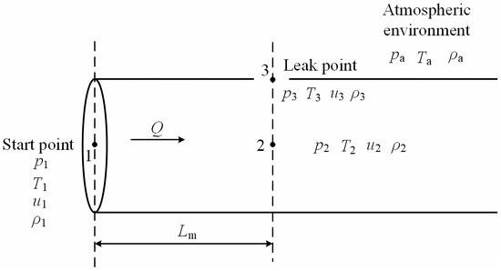
Figure 1. Schematic diagram of the gas pipe leakage process.

Assuming the gas behaves ideally, the pipeline flow is adiabatic, and the flow at the leakage hole is one-dimensional and isentropic, the leakage rate is given by the following:

$$Q=C_{0}A{P}_2\sqrt{{\displaystyle \frac{2M}{ZR{T}_2}}{\displaystyle \frac{k}{k-1}}\left[{({\displaystyle \frac{P_3}{P_2}})}^{{\displaystyle \frac{2}{k}}}-{({\displaystyle \frac{P_a}{P_2}})}^{{\displaystyle \frac{k+1}{k}}}\right]}$$

(7)

The magnitude of gas leakage rate at the leak hole depends on whether the gas at the hole is in critical flow or non-critical flow, determined by the critical pressure ratio (CPR) [22]. The expression is as follows:

$$CPR={\displaystyle \frac{P_c}{P_2}}={({\displaystyle \frac{2}{k+1}})}^{{\displaystyle \frac{k}{k-1}}}$$

(8)

When $P_a/P_2>CPR$, the leakage is considered subcritical flow. The leakage rate can be expressed as follows:

$$Q=C_{0}A{P}_2\sqrt{{\displaystyle \frac{2M}{ZR{T}_2}}{\displaystyle \frac{k}{k-1}}\left[{({\displaystyle \frac{P_a}{P_2}})}^{{\displaystyle \frac{2}{k}}}-{({\displaystyle \frac{P_a}{P_2}})}^{{\displaystyle \frac{k+1}{k}}}\right]}$$

(9)

When $P_a/P_2\le CPR$, the leakage is considered critical flow. The leakage rate can be expressed as follows:

$$Q=C_{0}A{P}_2\sqrt{{\displaystyle \frac{Mk}{ZR{T}_2}}{({\displaystyle \frac{2}{k+1}})}^{{\displaystyle \frac{k+1}{k-1}}}}$$

(10)

where $Q$ represents the leakage rate of gas, $A$ represents the area of the leakage hole, $M$ represents the molar mass of gas, $P_2$ and $P_3$ are the pressures at points 2 and 3, $P_a$ represents external environmental pressure, $P_c$ represents the critical pressure, $Z$ represents the compressibility factor, $k$ represents the energy dissipation function, and is usually 1.334 for gases composed of polyatomic molecules, and $C_0$ represents the energy dissipation function. In this study, the leakage hole is assumed to be circular with a regular geometric shape. To simplify the model and reduce uncertainty, a discharge coefficient of 1.0 is used. This represents an ideal case and provides a conservative, worst-case estimate of leakage and dispersion.

3. Numerical Model

3.1. Model Establishment

This study focuses on the small-hole circular leakage model, based on the GB5838-2015 standard [23]. The gas cabin is 2.0 m wide and 3.8 m high, with a DN500 medium-pressure gas pipeline (Shandong Zhuoyue Pipe Industry Co., Ltd., Linyi, China) installed within the pipe gallery. The pipe center is 0.6 m above the floor, and the distances from the pipeline to the left and right sidewalls are 0.6 m and 0.9 m, respectively. The inlet and outlet are square with dimensions of 1.0 m × 1.0 m. The longitudinal length of the model is 200 m, as shown in Figure 2. The geometry was created using the GAMBIT pre-processor (ANSYS, Inc., Canonsburg, PA, USA) (Figure 3). Methane was selected as the leaking gas. Its physical properties are listed in Table 1. The simulation was performed using the finite volume method, with a second-order upwind discretization scheme. Solver and model configurations are summarized in Table 2.

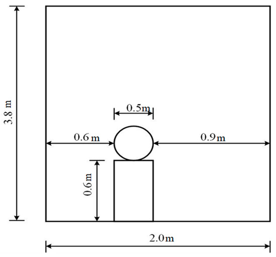
Figure 2. Gas tank section view.

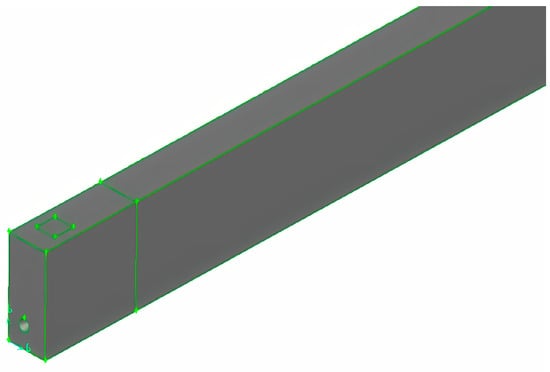
Figure 3. Schematic diagram of the GAMBIT model.

Table 1. Physical properties of methane.

Gas Type	Density $\mathit{\rho }$ (kg·m−3)	Specific Heat at Constant Pressure ${\mathit{C}}_{\mathit{P}}$ (J·kg−1·K−1)	$\mathbf{Adiabatic} \mathbf{Index} \mathit{k}$	$\mathbf{Dynamic} \mathbf{Viscosity} \mathit{\mu }$ (Pa·s)	Heat Transfer Coefficient $\mathit{\lambda }$ (W·m−1·K)	$\mathbf{Molar} \mathbf{Mass} \mathit{M}$ (g·mol−1)
Methane	0.6597	2237.2	1.306	1.111 × 10−5	0.03302	16.04

Table 2. ANSYS (2023 R2) Fluent solution settings.

Parameter	Settings
Gravity	0 (X); 0 (Y); −9.81 m/s2 (Z)
Turbulence model	standard k-ε model; considering buoyancy effects
Near-wall treatment	standard wall function
Pressure-velocity coupling	SIMPLE algorithm
Momentum spatial discretization	second-order upwind
Gradient spatial discretization	least squares cell
Pressure spatial discretization	Second-order scheme

3.2. Simulation Settings

The leakage hole is positioned at the center of the gas pipeline. The boundary condition is set as a mass-flow-inlet, and the mass flow rate is computed using a MATLAB (R2022a9.12.0) script. According to Equation (8), the critical pressure ratio (CPR) is calculated as 0.548. In this study, with $P_0/P=0.1/0.8=0.125<CRP$, the flow through the leakage hole is classified as subcritical. For different operational pipeline pressures, the initial pressure at the leakage hole (when the gas velocity reaches sonic speed) is shown in Table 3.

Table 3. Initial pressure at the leakage hole.

Pipeline Pressure (MPa)	Initial Pressure (MPa)
0.4	0.274
0.8	0.493
1.2	0.713
1.4	0.822
1.6	0.932

When ventilation effects are neglected, pressure-outlet boundary conditions are applied at the inlet and outlet.

The leakage hole size classification is defined in Table 4.

Table 4. Leakage aperture size and classification.

Leakage Aperture Type	Aperture Range (mm)
Minitype	0~1/4
Mesotype	1/4~2
Large	2~6
Rupture	>6

3.3. Measuring Point Layout

Gas concentration is monitored at intervals of 15 m along the pipeline, as shown in Figure 4, with coordinates listed in Table 5. Additionally, an extra measuring point (8*) is added at 7.5 m downstream from the leakage location.

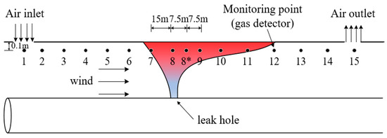
Figure 4. Schematic diagram of a gas detector.

Table 5. Monitoring point numbers and location coordinates.

Test Point	1	2	3	4	5	6	7	8
X (m)	0.85	0.85	0.85	0.85	0.85	0.85	0.85	0.85
Y (m)	2	10	25	40	55	70	85	100
Z (m)	3.7	3.7	3.7	3.7	3.7	3.7	3.7	3.7
Test point	8*	9	10	11	12	13	14	15
X (m)	0.85	0.85	0.85	0.85	0.85	0.85	0.85	0.85
Y (m)	107.5	115	130	145	160	175	190	198
Z (m)	3.7	3.7	3.7	3.7	3.7	3.7	3.7	3.7

3.4. Mesh Generation and Grid Sensitivity Analysis

Mesh generation involves domain decomposition. Unstructured grids using the T-grid method are applied around the inlet, outlet, and leakage hole with local refinement. The inlet and outlet are discretized using the Successive Ratio method with an interval of 0.1 (Figure 5a,b), while the leakage hole uses a finer mesh with an interval of 0.01 (Figure 5c,d). Other regions use the Cooper scheme for structured grids, also with an interval of 0.1.

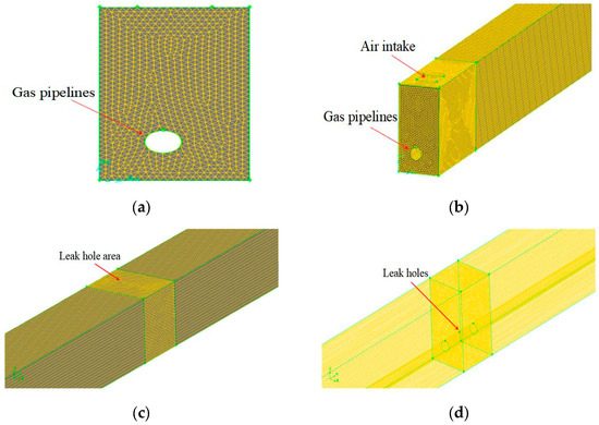
Figure 5. Schematic diagram of mesh division: (a) cross-section view; (b) inlet local refinement; (c) leakage hole local refinement; and (d) 3D view of refined region near the hole.

To verify the grid sensitivity, a case study was conducted using a leakage aperture of 5 mm and an operating pressure of 0.8 MPa. Five mesh configurations were generated using GAMBIT, containing 1,736,699, 2,276,343, 2,886,938, 3,843,760, and 5,203,709 cells, respectively. Analysis revealed that the simulation results at Monitoring Point 8 (positioned directly above the leakage hole) exhibited significant deviation when the grid size was 1,736,699. However, when the number of cells exceeded 2,276,343, the methane mass fraction began to stabilize at approximately 0.016, indicating numerical convergence. For Monitoring Points 8* and 9, the variation remained within 5% across all grid sizes, demonstrating consistent accuracy and mesh independence. Considering the trade-off between computational efficiency and result precision, the mesh with 3,843,760 cells was selected for the final simulation. Figure 6 presents the time-history curves of methane concentration at each monitoring point under the five mesh densities.

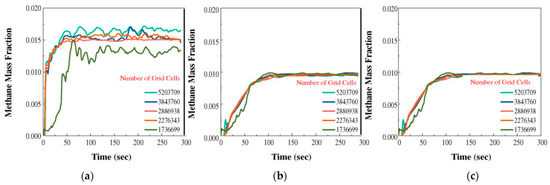
Figure 6. Grid independence verification at (a) Monitoring Point 8, (b) Monitoring Point 8*, and (c) Monitoring Point 9. The methane mass fraction results converge when the number of grid cells exceeds 2,276,343, with deviations between medium and fine grids remaining below 5%. A grid size of 3,843,760 cells was selected for all subsequent simulations to ensure a balance between accuracy and computational efficiency.

3.5. Model Verification

Due to the high cost and inherent safety risks associated with on-site experiments, this study adopts the gas leakage test conducted by Liu [24] to verify the validity of the numerical simulation. The boundary conditions are consistent with those of the numerical model, using a leakage size of 0.16 mm and a mass flow rate of 1.587 × 10⁻⁴ kg/s. Figure 7a,b presents a comparison between the experimental and simulated methane mass fractions at sampling points 9 and 1 during the test. As shown in Figure 7, a significant discrepancy exists between the experimental and simulated methane mass fractions during the early stage of leakage. This difference arises because numerical simulations typically assume that a stable mass flow rate is established immediately upon leakage. In reality, however, the initial leakage phase may involve a ramp-up or fluctuation in flow rate, causing the experimental results to deviate from the steady-state assumption of the simulation. As the leakage duration increases, the experimental and simulated values exhibit similar trends and gradually converge to a constant. The average errors at sampling points 9 and 1 are 12.9% and 10.7%, respectively. These deviations are primarily attributed to the proximity of the sampling points to the leakage source or their location within complex airflow regions, making them more susceptible to errors introduced by the turbulence model. In conclusion, the CFD simulation results are generally in good agreement with the experimental data, confirming the accuracy and reliability of the numerical model in predicting gas leakage and diffusion processes within underground utility tunnels.

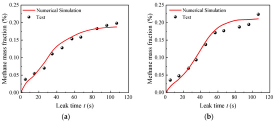
Figure 7. Comparison chart between test and numerical simulation: (a) sampling point 1 and (b) sampling point 9.

3.6. Simulation Scenarios

The small-hole leakage model was simulated under varying conditions of leakage aperture and pipeline operating pressure. The details of the simulation conditions are presented in Table 6.

Table 6. Simulation condition settings.

Leakage Condition	$\mathbf{Leakage} \mathbf{Size} \mathit{d}$ (mm)	$\mathbf{Operating} \mathbf{Pressure} \mathit{P}$(MPa)	$\mathbf{Mass} \mathbf{Flow} \mathbf{Rate} \mathit{Q}$(kg/s)	$\mathbf{Ventilation} \mathbf{Exchange} \mathbf{Rate} \mathit{N}$(Times/h)	$\mathbf{Temperature} \mathit{T}$ (°C)	$\mathbf{Relative} \mathbf{Humidity} \mathit{H}$ (%)
1	4	0.8	0.019	6/12	15	70%
2	5	0.8	0.030	6/12	15	70%
3	6	0.8	0.044	6/12	15	70%
4	8	0.8	0.066	6/12	15	70%
5	10	0.8	0.103	6/12	15	70%
6	5	0.4	0.017	6/12	15	70%
7	5	1.2	0.040	6/12	15	70%
8	5	1.4	0.045	6/12	15	70%
9	5	1.6	0.057	6/12	15	70%

4. Influence of Leak Sources on Gas Dispersion

4.1. Interactions of Gas Leak Parameters

This study analyzes the mutual influence of gas leakage parameters for different leakage apertures of 4, 5, 6, 8, and 10 mm, as well as pipeline operating pressures of 0.4, 0.8, 1.2, 1.4, and 1.6 MPa. Figure 8a illustrates the relationship between leakage rate and leakage aperture under various pipeline operating pressures. The result shows that when the pipeline operating pressure is consistent, the leakage rate increases according to a power-law relationship with the leakage aperture. For instance, at a pipeline operating pressure of 1.2 MPa, the leakage rate increases by 0.55 times within the 4~6 mm aperture range, and by 0.8 times within the 6~8 mm aperture range. Additionally, higher pipeline operating pressures lead to higher leakage rates for the same leakage aperture. For a 4 mm leakage aperture, the difference in leakage rates under various pipeline operating pressures is relatively small, all below 0.040 kg/s. However, when the leakage aperture increases to 10 mm, the difference in leakage rates under different pipeline operating pressures becomes significant, ranging from 0.051 to 0.206 kg/s.

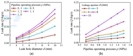
Figure 8. (a) Relationship between leakage rate and leakage aperture under different pipe pressures; (b) Relationship between leakage rate and pipe pressure under different leakage apertures.

Figure 8b illustrates the relationship between leakage rate and pipeline operating pressure for different leakage apertures. From the figure, it is evident that the leakage rate varies linearly with the pipeline operating pressure for the same leakage aperture. When the leakage aperture is 8 mm, the leakage rate increases by a factor of 1 for pipeline operating pressures ranging from 0.4 to 1.6 MPa. Additionally, larger leakage apertures result in faster leakage rates for the same pipeline operating pressure. For instance, at a pipeline operating pressure of 0.4 MPa, the leakage rate is below 0.025 for leakage apertures between 4 and 6 mm, while it increases from 0.019 to 0.051 for leakage apertures between 6 and 10 mm.

4.2. Influence of Different Leak Apertures

4.2.1. Methane Concentration Change

Figure 9a–f represents the curves of methane mass fraction at various monitoring points under different leakage apertures as a function of leakage time. From the figure, it can be observed that the methane mass fraction initially increases with leakage time and then tends to stabilize. The time required to reach stability increases with the longitudinal distance from the leakage orifice, with monitoring points 8*, 11, and 13 reaching stability after 50, 80, and 125 s, respectively. At the same monitoring point, the methane mass fraction increases with the leakage aperture diameter, while at different monitoring points, the methane mass fraction remains the same when the same leakage aperture diameter reaches stability. This is because large-aperture jets have higher initial momentum and penetration capacity, which can carry more methane to downstream monitoring points, resulting in an increase in the concentration at the same monitoring point as the aperture increases. For instance, at different monitoring points, the methane mass fractions for leakage apertures of 4, 6, and 10 mm are 0.003, 0.007, and 0.016, respectively. Furthermore, when the leakage apertures are 4 and 5 mm, none of the monitoring points reach the required concentration for alarm under longitudinal ventilation conditions.

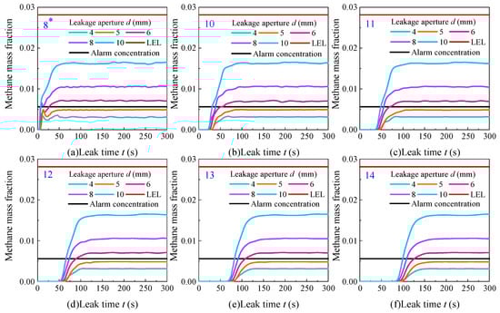
Figure 9. Effect of leakage aperture on methane mass fraction at different measuring points: (a) 8*; (b) 10; (c) 11; (d) 12; (e) 13; and (f) 14.

4.2.2. Impact on Alarm Time

Figure 10 depicts the alarm time at different monitoring points for leakage apertures of 6, 8, and 10 mm. From the figure, it can be observed that under different leakage aperture diameters, the alarm time exhibits a linear increase with the longitudinal distance from the leakage orifice. At the same location, the alarm time decreases with the leakage aperture. For instance, at monitoring point 8*, the alarm times corresponding to leakage apertures of 6, 8, and 10 mm are 26.88, 7.47, and 6.81 s, respectively. At monitoring point 12, the alarm times are 89.95, 73.62, and 66.05 s, respectively, for the same leakage aperture diameters. Linear fitting is performed on the alarm time under different leakage apertures, and the fitting results are shown in Table 7.

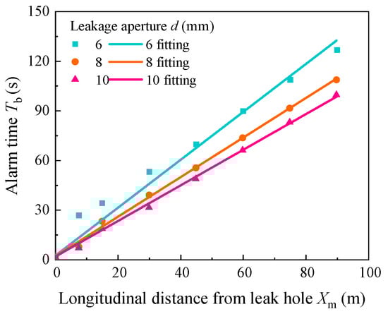
Figure 10. Relationship between alarm time and longitudinal distance from the leak hole under different leakage apertures.

Table 7. Expressions of alarm time relationship under different leakage apertures.

$\mathbf{Leakage} \mathbf{Aperture} \mathit{d}$ (mm)	Relational Expression	$\mathbf{The} \mathbf{Maximum} \mathbf{Alarm} \mathbf{Spacing} {\mathit{X}}_{\mathit{m}}$ (m)
		Alarm Time 30 s	Alarm Time 60 s	Alarm Time 90 s	Alarm Time 120 s
6 mm	${\mathit{T}}_{\mathit{b}}=\mathbf{1.45}{\mathit{X}}_{\mathit{m}}+\mathbf{2.10}$	19.24	39.93	60.62	81.31
8 mm	${\mathit{T}}_{\mathit{b}}=\mathbf{1.20}{\mathit{X}}_{\mathit{m}}+\mathbf{1.70}$	23.58	48.58	73.58	98.58
10 mm	${\mathit{T}}_{\mathit{b}}=\mathbf{1.08}{\mathit{X}}_{\mathit{m}}+\mathbf{1.50}$	26.39	54.17	81.94	109.72

4.2.3. Longitudinal Distribution of Methane

Figure 11a–f shows the influence of the leakage aperture on the longitudinal distribution of methane concentration at different leakage times. From the figure, when leakage time and position are constant, the methane mass fraction increases with the leakage aperture. Simultaneously, regions of high methane concentration expand with increasing leakage time. However, at a longitudinal position of approximately 200 m, there is a sudden decrease in methane mass fraction. This could be due to its proximity to the exhaust vent, causing the leaked methane gas to exit into the atmosphere through the vent after the leakage.

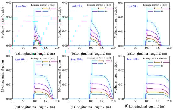
Figure 11. Effect of leakage aperture on longitudinal distribution of methane concentration under different leakage times: (a) Leak 20 s; (b) Leak 40 s; (c) Leak 60 s; (d) Leak 80 s; (e) Leak 100 s; and (f) Leak 120 s.

4.2.4. Influence on Methane Dispersion Distance

Figure 12 shows the relationship between methane dispersion distance and leakage time for various leakage apertures. From the figure, for different leakage apertures, the methane dispersion distance shows a linear increase with leakage time. When the leakage time is constant, the methane dispersion distance increases with the enlargement of the leakage aperture. For a leakage time of 20 s, the methane dispersion distances for apertures of 4, 6, and 10 mm are 20.56, 24.66, and 28.86 m, respectively. Correspondingly, for a leakage time of 80 s, the methane dispersion distances are 75.39, 79.29, and 87.09 m, respectively. In addition, linear fitting was conducted for methane gas dispersion distances under different leakage apertures, and the fitting results are shown in Table 8.

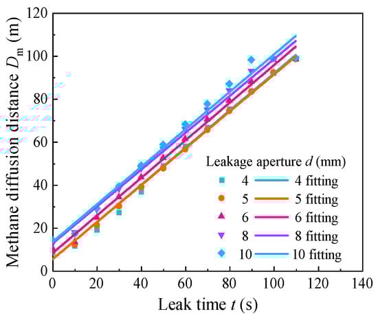
Figure 12. Changes in methane diffusion distance with leakage time under different leakage apertures.

Table 8. Relationship expression of methane gas diffusion distance under different leakage apertures.

$\mathbf{Leakage} \mathbf{Aperture} \mathit{d}$ (mm)	Relational Expression $(\mathit{t}\ge 1\mathbf{ s})$	$\mathbf{Leakage} \mathbf{Time} \mathit{t}$ (s)
		Dispersion Distance 30 m	Dispersion Distance 50 m	Dispersion Distance 70 m	Dispersion Distance 90 m
4 mm	${\mathit{D}}_{\mathit{m}}=\mathbf{0.86}\mathit{t}+\mathbf{4.20}$	30.00	53.26	76.51	99.77
5 mm	${\mathit{D}}_{\mathit{m}}=\mathbf{0.86}\mathit{t}+\mathbf{5.04}$	29.02	52.28	75.53	98.79
6 mm	${\mathit{D}}_{\mathit{m}}=\mathbf{0.88}\mathit{t}+\mathbf{5.23}$	28.15	50.88	73.60	96.33
8 mm	${\mathit{D}}_{\mathit{m}}=\mathbf{0.91}\mathit{t}+\mathbf{6.14}$	26.22	48.20	70.18	92.15
10 mm	${\mathit{D}}_{\mathit{m}}=\mathbf{0.92}\mathit{t}+\mathbf{6.30}$	25.76	47.50	69.24	90.98

4.2.5. Influence of Leak Aperture Size on Methane Backflow Length

The leakage aperture is a normalized dimensionless quantity. Figure 13 shows the relationship curve between the dimensionless methane backflow length and $\mathit{d}/\mathit{D}$. From the figure, the methane upstream length increases with the leakage aperture. This could be attributed to the increase in the leakage aperture and the total methane leakage amount within the same timeframe, leading to an increase in the backflow length. For dimensionless leakage apertures of 0.008, 0.012, and 0.020, the corresponding dimensionless methane backflow lengths are 0.31, 0.44, and 0.67, respectively. Additionally, through fitting, it was found that the methane backflow length increases with the leakage aperture to the power of 0.83. The fitting result is presented in Equation (11).

$$l^{*}=16.40{({\displaystyle \frac{d}{D}})}^{0.83}$$

(11)

where ${\mathit{l}}^{\mathit{*}}$ represents the dimensionless backflow length, $\mathit{d}$ represents the leakage aperture, and $\mathit{D}$ represents the pipe diameter.

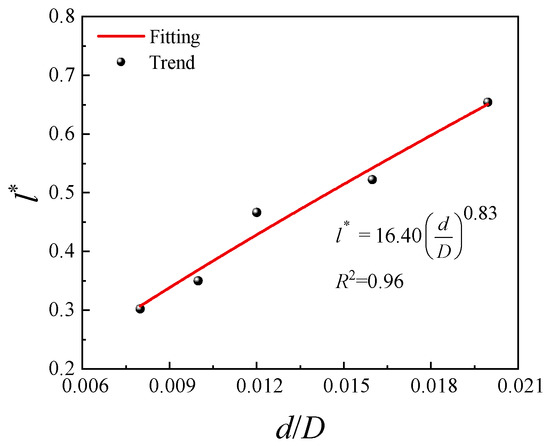
Figure 13. Effect of leakage aperture on methane backflow length.

4.3. Different Pipeline Operating Pressures

4.3.1. Changes in Methane Concentration

Figure 14a–f displays the curves of methane mass fraction variation over time at different measurement points under various pipeline operating pressures. From the figure, the methane mass fraction initially increases with leakage time before stabilizing. At pipeline operating pressures of 0.4, 0.8, and 1.6 MPa, the methane mass fractions at each measurement point are similar, measuring 0.0027, 0.0047, and 0.0091, respectively. Additionally, when the leakage time is constant, the methane mass fraction increases with the rise in pipeline operating pressure.

Figure 14. Effect of pipeline pressure on methane mass fraction at different measuring points: (a) 8*; (b) 10; (c) 11; (d) 12; (e) 13; and (f) 14.

4.3.2. Impact on Alarm Time

Figure 15 depicts the relationship between longitudinal distance from the leakage hole and alarm time under different pipeline operating pressures. From the figure, under various pipeline operating pressures, there is a linear increase in alarm time with longitudinal distance from the leakage hole. At the same position relative to the leakage source, alarm time decreases with increasing pipeline operating pressure. For instance, at a distance of 30 m from the leakage source, the alarm time for pipeline operating pressures of 1.2, 1.4, and 1.6 MPa is 64.77, 54.88, and 46.29 s, respectively. Similarly, at a distance of 75 m from the leakage source, the corresponding alarm times are 124.03, 108.80, and 102.18 s, respectively. Additionally, the fitting results are presented in Table 9.

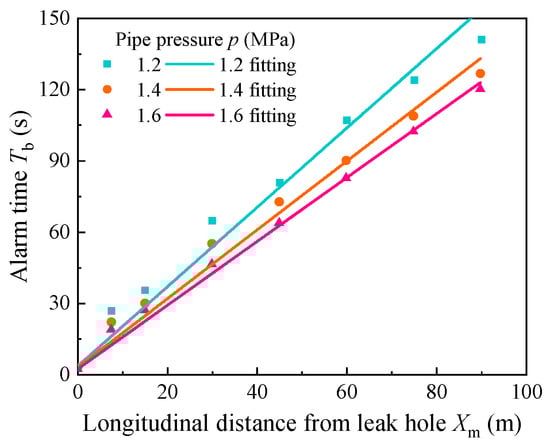
Figure 15. Relationship between alarm time and longitudinal distance from the leak hole under different pipeline pressures.

Table 9. Expression of alarm time relationship under different pipeline pressures.

$\mathbf{Pipeline} \mathbf{Pressure} \mathit{P}$(MPa)	Relational Expression	$\mathbf{The} \mathbf{Maximum} \mathbf{Alarm} \mathbf{Spacing} {\mathit{X}}_{\mathit{m}}$ (m)
		Alarm Time 30 s	Alarm Time 60 s	Alarm Time 90 s	Alarm Time 120 s
1.2	${\mathit{T}}_{\mathit{b}}=\mathbf{1.67}{\mathit{X}}_{\mathit{m}}+\mathbf{3.2}$	16.05	34.01	51.98	69.94
1.4	${\mathit{T}}_{\mathit{b}}=\mathbf{1.45}{\mathit{X}}_{\mathit{m}}+\mathbf{2.6}$	18.90	39.59	60.28	80.97
1.6	${\mathit{T}}_{\mathit{b}}=\mathbf{1.34}{\mathit{X}}_{\mathit{m}}+\mathbf{1.9}$	20.97	43.36	65.75	88.13

4.3.3. Longitudinal Distribution of Methane Concentration

Figure 16a–f shows the influence of pipeline operating pressure on the longitudinal distribution of methane concentration under different leakage durations. From the figure, the overall methane dispersion area increases with pipeline operating pressure. Additionally, at the same distance from the leakage source and for identical leakage durations, higher pipeline operating pressures correspond to higher methane mass fractions. For instance, at a distance of 25 m from the leakage source and a leakage duration of 60 s, methane mass fractions for pipeline operating pressures of 0.4, 1.2, and 1.6 MPa are 0.0025, 0.006, and 0.008, respectively. Similarly, for a leakage duration of 100 s, corresponding methane mass fractions are 0.003, 0.006, and 0.009, respectively. Additionally, the maximum methane mass fraction increases initially with leakage duration before stabilizing. At a leakage duration of 120 s, the pipeline operating pressures of 0.4, 1.2, and 1.6 MPa correspond to maximum methane mass fractions of 0.011, 0.013, and 0.016, respectively.

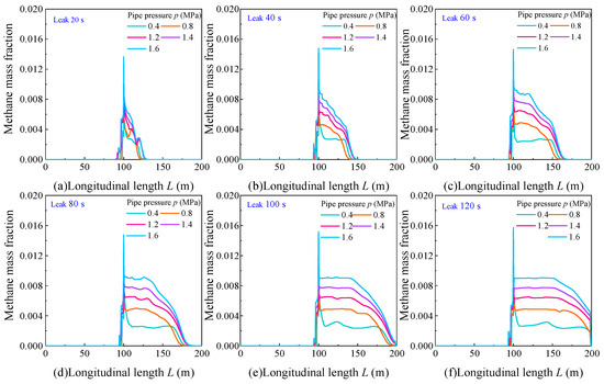
Figure 16. Effect of pipeline operating pressure on longitudinal distribution of methane concentration at different times: (a) Leak 20 s; (b) Leak 40 s; (c) Leak 60 s; (d) Leak 80 s; (e) Leak 100 s; and (f) Leak 120 s.

4.3.4. Influence on Methane Dispersion Distance

Figure 17 shows the relationship between methane dispersion distance and leakage time under different pipeline operating pressures. From the figure, under various pipeline operating pressures, the methane gas dispersion distance shows a linear increase with leakage time. At the same leakage time, the methane dispersion distance increases with pipeline operating pressure. For instance, at a leakage time of 30 s, the methane gas dispersion distances for pipeline operating pressures of 0.4, 1.2, and 1.6 MPa are 30.07, 36.97, and 39.67 m, respectively. Similarly, at a leakage time of 60 s, the corresponding methane gas dispersion distances are 56.68, 64.68, and 67.78 m, respectively. Additionally, the fitting expressions are presented in Table 10.

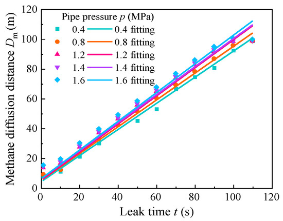
Figure 17. Changes in leakage diffusion distance with time under different pipeline pressures.

Table 10. Relationship of methane gas diffusion distance under different operating pressures.

$\mathbf{Pipeline} \mathbf{Pressure} \mathit{P}$(MPa)	Relational Expression $(\mathit{t}\ge 1\mathit{ s})$	$\mathbf{Leakage} \mathbf{Time} \mathit{t}$ (s)
		Dispersion Distance 30 m	Dispersion Distance 50 m	Dispersion Distance 70 m	Dispersion Distance 90 m
0.4	${\mathit{D}}_{\mathit{m}}=\mathbf{0.86}\mathit{t}+\mathbf{4.99}$	29.08	52.34	75.59	98.85
0.8	${\mathit{D}}_{\mathit{m}}=\mathbf{0.86}\mathit{t}+\mathbf{5.04}$	29.02	52.27	75.53	98.79
1.2	${\mathit{D}}_{\mathit{m}}=\mathbf{0.94}\mathit{t}+\mathbf{5.13}$	26.46	47.73	69.01	90.29
1.4	${\mathit{D}}_{\mathit{m}}=\mathbf{0.94}\mathit{t}+\mathbf{6.08}$	25.45	46.72	68.00	89.28
1.6	${\mathit{D}}_{\mathit{m}}=\mathbf{0.96}\mathit{t}+\mathbf{6.15}$	24.84	45.68	66.51	87.34

4.3.5. Influence of Pipeline Operating Pressure on Methane Backflow Length

Using atmospheric pressure $P_a$ as a reference, the pipeline operating pressure is a normalized dimensionless quantity. Figure 18 illustrates the effect of dimensionless pipeline operating pressure on the dimensionless methane backflow length. From the figure, the methane backflow length increases with pipeline operating pressure. For dimensionless pipeline operating pressures of 3.95, 11.84, and 15.79, the corresponding dimensionless methane backflow lengths are 0.24, 0.44, and 0.56, respectively. Nonlinear fitting between the two variables reveals that the methane backflow length is proportional to the pipeline operating pressure raised to the power of 0.63, as described in Equation (12).

$$l^{*}=0.09{({\displaystyle \frac{P}{P_a}})}^{0.63}$$

(12)

where $l^{*}$ represents the dimensionless backflow length, $P$ represents the pipeline operating pressure, and $P_a$ represents the atmospheric pressure.

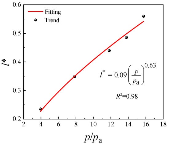
Figure 18. Effect of pipeline operating pressure on methane backflow length.

4.4. Establishment of Prediction Models for Leak Dispersion Parameters

4.4.1. Prediction Model for Alarm Time

Taking into account the influence of leakage aperture, pipeline operating pressure, and longitudinal distance from the leakage hole on alarm time, Figure 19a presents the predictive model for alarm time of small aperture leaks in an underground comprehensive pipe gallery. The specific expression is shown in Equation (13), with a coefficient of determination R² = 0.97. The absolute residuals between the theoretical model calculation values and numerical simulation values are depicted in Figure 19b, with an average residual of 2.53 across all points, indicating a good overall fit. The prediction accuracy of the model is highly dependent on the reliability of the CFD simulation. In order to ensure the credibility of the results, the computational domain needs to be optimized by grid independence verification, and the key coefficients in the model need to be recalibrated after adjusting the grid to match the updated flow field data.

$$T_b=-464.27\left({\displaystyle \frac{d}{D}}\right)\left({\displaystyle \frac{P}{P_a}}\right)+2.94\left({\displaystyle \frac{P}{P_a}}\right)+1.22X_m+40.97$$

(13)

where $T_b$ represents the alarm time, $d$ represents the leakage aperture, $P$ represents the pipeline operating pressure, $P_a$ represents the atmospheric pressure, and $X_m$ represents the longitudinal distance from the leakage hole.

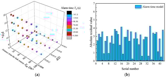
Figure 19. (a) The impact of different factors on alarm time; (b) prediction model and numerical simulation residual diagram.

4.4.2. Prediction Model for Methane Dispersion Distance

Figure 20a depicts the predictive model for methane dispersion distance under small aperture leaks in an underground comprehensive pipe gallery. The fitting expression is shown in Equation (14), with a coefficient of determination R² = 0.98. The specific residuals are illustrated in Figure 20b, revealing an average residual of 1.97, which indicates a good fit.

$$D_m=79.65\left({\displaystyle \frac{d}{D}}\right)\left({\displaystyle \frac{P}{P_a}}\right)-0.02\left({\displaystyle \frac{P}{P_a}}\right)+0.86t+0.76$$

(14)

where $D_m$ represents methane dispersion distance, and $t$ represents leakage time.

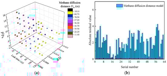
Figure 20. (a) Effects of different factors on methane diffusion distance; (b) prediction model and numerical simulation residual diagram.

5. Conclusions

In this study, CFD simulation is used to establish a refined model for gas leaks in the comprehensive pipe gallery, and the influence of leakage aperture and pipeline operating pressure on gas leakage and diffusion is analyzed. Furthermore, it explores the diffusion law of gas leaks by analyzing alarm time, methane diffusion distance, and backflow length. The study also proposes corresponding prediction models for leak dispersion parameters, aiming to provide a foundation for predicting hazardous areas following gas leaks in the comprehensive pipe gallery. The following key conclusions were drawn:

(1)

When the operating pressure of the pipeline remains constant, the leakage rate increases according to a power-law relationship with the leakage aperture size. Conversely, when the leakage aperture size is constant, the leakage rate exhibits a linear relationship with the pipeline operating pressure. Specifically, when the leakage aperture size is 8 mm, and the pipeline operating pressure ranges from 0.4 to 1.6 MPa, the leakage rate doubles uniformly.

(2)

The alarm time decreases with the increase in both the leakage aperture and pipeline operating pressure. Meanwhile, the methane diffusion distance increases with the increase in these two factors. Additionally, the methane backflow length increases according to a power-law relationship with the dimensionless leakage aperture and pipeline operating pressure, showing exponents of 0.83 and 0.63, respectively.

(3)

A predictive model for alarm time and methane diffusion distance was established, with fitted correlation coefficients of 0.97 and 0.98, and average residuals at each point of 2.53 and 1.97, respectively.

This paper analyzes the influence of multiple factors on the diffusion of gas leakage, but does not consider the influence law under the coupling effect of multiple factors for the time being. Based on the on-site measured data, this paper studies the influence of internal environmental temperature and humidity on gas leakage and diffusion. The influence of temperature gradient and humidity gradient on gas leakage and diffusion is not considered for the time being, and further research can be conducted in the future.

References

- Wang, W.; Mao, X.; Liang, H.; Yang, D.; Zhang, J.; Liu, S. Experimental research on in-pipe leaks detection of acoustic signature in gas pipelines based on the artificial neural network. Measurement 2021, 183, 109875. [Google Scholar] [CrossRef]
- Li, X.; Zhang, Y.; Abbassi, R.; Yang, M.; Zhang, R.; Chen, G. Dynamic probability assessment of urban natural gas pipeline accidents considering integrated external activities. J. Loss Prev. Process Ind. 2021, 69, 104388. [Google Scholar] [CrossRef]
- Valdenebro, J.V.; Gimena, F.N. Urban utility tunnels as a long-term solution for the sustainable revitalization of historic centres: The case study of Pamplona-Spain. Tunn. Undergr. Space Technol. 2018, 81, 228–236. [Google Scholar] [CrossRef]
- Xu, D.; Li, Y.; Yang, X. Enhancing Resilience in Urban Utility Tunnels Power Transmission Systems: Analysing Temperature Distribution in near-Wall Cable Fires for Risk Mitigation. Tunn. Undergr. Space Technol. 2024, 152, 105911. [Google Scholar] [CrossRef]
- Wang, Q.; Wang, B.; Palacios, A.; Yao, Y. Investigation of the Possible Use of Sound Waves for Fire Safety in Tunnels: A Fundamental Study on Flame Dynamics and the Extinguishment Criteria of Gas Leak Jet Fires. Tunn. Undergr. Space Technol. 2025, 162, 106663. [Google Scholar] [CrossRef]
- Li, Y.; Qian, X.; Zhang, S.; Sheng, J.; Hou, L.; Yuan, M. Assessment of gas explosion risk in underground spaces adjacent to a gas pipeline. Tunn. Undergr. Space Technol. 2023, 131, 104785. [Google Scholar] [CrossRef]
- Wang, W.; Zhang, Y.; Li, Y.; Hu, Q.; Liu, C.; Liu, C. Vulnerability analysis method based on risk assessment for gas transmission capabilities of natural gas pipeline networks. Reliab. Eng. Syst. Saf. 2022, 218, 108150. [Google Scholar] [CrossRef]
- Bonnaud, C.; Cluzel, V.; Corcoles, P.; Dubois, J.P.; Louvet, V.; Maury, M.; Poenou, J. Experimental study and modelling of the consequences of small leaks on buried transmission gas pipeline. J. Loss Prev. Process Ind. 2018, 55, 303–312. [Google Scholar] [CrossRef]
- Gao, B.; Mitton, M.K.; Bell, C.; Zimmerle, D.; Deepagoda, T.C.; Hecobian, A.; Smits, K.M. Study of methane migration in the shallow subsurface from a gas pipe leak. Elem. Sci. Anthr. 2021, 9, 00008. [Google Scholar] [CrossRef]
- Zhou, Z.; Zhang, J.; Huang, X.; Zhang, J.; Guo, X. Trend of soil temperature during pipeline leakage of high-pressure natural gas: Experimental and numerical study. Measurement 2020, 153, 107440. [Google Scholar] [CrossRef]
- Tian, Y.; Qin, C.; Yang, Z.; Hao, D. Numerical simulation study on the leakage and diffusion characteristics of high-pressure hydrogen gas in different spatial scenes. Int. J. Hydrogen Energy 2024, 50, 1335–1349. [Google Scholar] [CrossRef]
- Wang, L.; Chen, J.; Ma, T.; Ma, R.; Bao, Y.; Fan, Z. Numerical study of leakage characteristics of hydrogen-blended natural gas in buried pipelines. Int. J. Hydrogen Energy 2024, 49, 1166–1179. [Google Scholar] [CrossRef]
- Li, F.; Yuan, Y.; Yan, X.; Malekian, R.; Li, Z. A study on a numerical simulation of the leakage and diffusion of hydrogen in a fuel cell ship. Renew. Sustain. Energy Rev. 2018, 97, 177–185. [Google Scholar] [CrossRef]
- Qian, J.Y.; Li, X.J.; Gao, Z.X.; Jin, Z.J. A numerical study of hydrogen leakage and diffusion in a hydrogen refueling station. Int. J. Hydrogen Energy 2020, 45, 14428–14439. [Google Scholar] [CrossRef]
- Ebrahimi-Moghadam, A.; Farzaneh-Gord, M.; Arabkoohsar, A.; Moghadam, A.J. CFD analysis of natural gas emission from damaged pipelines: Correlation development for leakage estimation. J. Clean. Prod. 2018, 199, 257–271. [Google Scholar] [CrossRef]
- Zeng, F.; Jiang, Z.; Zheng, D.; Si, M.; Wang, Y. Study on numerical simulation of leakage and diffusion law of parallel buried gas pipelines in tunnels. Process Saf. Environ. Prot. 2023, 177, 258–277. [Google Scholar] [CrossRef]
- Kang, Y.; Ma, S.; Song, B.; Xia, X.; Wu, Z.; Zhang, X.; Zhao, M. Simulation of hydrogen leakage diffusion behavior in confined space. Int. J. Hydrogen Energy 2024, 53, 75–85. [Google Scholar] [CrossRef]
- Zhang, P.; Lan, H. Effects of ventilation on leakage and diffusion law of gas pipeline in utility tunnel. Tunn. Undergr. Space Technol. 2020, 105, 103557. [Google Scholar] [CrossRef]
- Ebrahimi-Moghadam, A.; Farzaneh-Gord, M.; Deymi-Dashtebayaz, M. Correlations for estimating natural gas leakage from above-ground and buried urban distribution pipelines. J. Nat. Gas Sci. Eng. 2016, 34, 185–196. [Google Scholar] [CrossRef]
- Xie, Y.; Liu, J.; Qin, J.; Xu, Z.; Zhu, J.; Liu, G.; Yuan, H. Numerical simulation of hydrogen leakage and diffusion in a ship engine room. Int. J. Hydrogen Energy 2024, 55, 42–54. [Google Scholar] [CrossRef]
- Dong, G.; Xue, L.; Yang, Y.; Yang, J. Evaluation of hazard range for the natural gas jet released from a high-pressure pipeline: A computational parametric study. J. Loss Prev. Process Ind. 2010, 23, 522–530. [Google Scholar] [CrossRef]
- Dormohammadi, R.; Farzaneh-Gord, M.; Ebrahimi-Moghadam, A.; Ahmadi, M.H. Heat transfer and entropy generation of the nanofluid flow inside sinusoidal wavy channels. J. Mol. Liq. 2018, 269, 229–240. [Google Scholar] [CrossRef]
- GB 50838-2015; Technical Specification for Urban Comprehensive Pipeline Corridor Engineering (In Chinese). China Planning Press: Beijing, China, 2015.
- Liu, X.X. Theoretical and Experimental Study of Gas Pipeline Leakage Diffusion in Comprehensive Pipeline Corridors (In Chinese). Master’s Thesis, Beijing University of Civil Engineering and Architecture, Beijing, China, 2018. [Google Scholar]
Disclaimer/Publisher’s Note: The statements, opinions and data contained in all publications are solely those of the individual author(s) and contributor(s) and not of MDPI and/or the editor(s). MDPI and/or the editor(s) disclaim responsibility for any injury to people or property resulting from any ideas, methods, instructions or products referred to in the content. |
© 2025 by the authors. Licensee MDPI, Basel, Switzerland. This article is an open access article distributed under the terms and conditions of the Creative Commons Attribution (CC BY) license (https://creativecommons.org/licenses/by/4.0/).