Abstract
The integration of renewable energy into distribution networks has led to voltage violations and increased network losses. Traditional control devices, with slow response, struggle to precisely control power flow in active distribution networks (ADNs). Optimizing from both supply and demand sides, an ADN power flow optimization method is proposed for accurate and dynamic power flow regulation to address these issues. On the demand side, the peak, valley, and flat periods are divided by the fuzzy transitive closure method. Balancing user satisfaction maximization and load fluctuation minimization, time-of-use (TOU) prices are solved by the non-dominated sorting genetic algorithm II (NSGA-II). On the supply side, operating cost and voltage deviation minimization are objectives, with a proposed optimization method coordinating precise continuous regulation devices and low-cost discrete ones. After second-order cone programming and linearization, the multi-objective model is solved via the normalized normal constraint (NNC) algorithm to get a solution set, from which the optimal solution is selected using Entropy Weight and Technique for Order Preference by Similarity to an Ideal Solution (EW-TOPSIS). The results indicate that, in comparison with the proposed method, ADN not implementing demand-side TOU pricing strategies exhibits an increase in operating costs by 13.83% and a rise in voltage deviation by 4.14%. Meanwhile, ADN utilizing only traditional discrete control devices demonstrates more significant increments, with operating costs increasing by 182.40% and voltage deviation rising by 113.02%.
1. Introduction
With the depletion of fossil fuels, the pace of developing renewable energy power generation is accelerating [1,2]. Renewable energy is increasingly integrated into distribution networks in the form of distributed generation (DG), thereby transforming traditional passive distribution networks into active distribution networks (ADN) that encompass energy collection, transmission, storage, and distribution [3]. The operation of ADN is more complex than those of traditional distribution networks [4,5]. The volatility of photovoltaic power generation and wind power generation leads to high frequency and large amplitude of power fluctuations in feeders connected to DG, causing problems such as voltage violations and increased network losses, and even seriously threatening the stability and safety of ADN operation [6,7,8].
The on-load tap changer (OLTC) and capacitor banks (CBs) are traditional devices used to regulate grid operation [9,10,11]. Due to the frequent fluctuations in renewable energy output, it is difficult to achieve fast and precise control of ADNs relying solely on OLTC and CBs, which have slow response speeds and limited operation times [12]. With the development of power electronic technology, the soft open point (SOP) has gradually replaced some tie switches in distribution networks [13,14]. The SOP can realize real-time and continuous regulation of cross-feeder power flow and voltage through precise power transmission [15,16,17]. Optimization methods for the coordinated operation of SOP and DGs are, respectively, proposed in [18,19], confirming that the integration of SOP can improve the power quality and renewable energy absorption rate of ADN. In addition, SOP can also enhance the operational flexibility of ADN from both temporal and spatial dimensions [20]. Therefore, SOPs are suitable for integration into ADNs to mitigate the impact of power fluctuations from renewable energy generation.
Due to the high investment cost of SOP devices, it is difficult to replace all traditional control and regulation devices in the system with SOP in current engineering applications [21]. Therefore, SOP can be operated in coordination with traditional control devices [22]. An optimization strategy for the coordinated operation of SOP, OLTC, tie switches, and an energy storage system was proposed in [23] to mitigate voltage fluctuations and reduce losses. Based on SOP and CBs, a bi-level optimization model considering both the economy and voltage level of distribution networks was constructed in [24] to achieve precise power flow control. Based on deep reinforcement learning, a dual-time-scale reactive power optimization strategy for the coordination of SOP, OLTC, and CB was proposed in [25], which featured good real-time performance and lower communication costs.
In the optimization of flexible interconnected distribution networks, most scholars tend to focus on operational optimization on the grid side, while few have conducted comprehensive optimization by combining both the supply and demand sides of loads. Demand response (DR) strategies play a role in stabilizing voltage and reducing costs in ADN [26,27]. Based on DR strategies, a market-based real-time congestion mitigation algorithm was proposed in [28] for ADN with dynamic electric vehicle charging behavior. In [29], a multi-objective coordination scheme was proposed for ADN based on DR strategies, which effectively reduced the peak–valley load difference and system operation costs. TOU pricing is a popular research strategy of DR. However, some studies are limited to establishing a single objective function for formulating TOU pricing strategies, such as only considering users’ electricity costs or load peak–valley differences [30,31,32,33]. The main goal of implementing TOU pricing strategies is to achieve peak shaving and valley filling of the load. Moreover, considering users’ electricity costs is actually a consideration of user satisfaction. Therefore, when formulating TOU pricing strategies, comprehensive consideration should be given to minimizing load fluctuations and maximizing users’ comprehensive satisfaction.
Some scholars only consider a single objective function when optimizing the operation of flexible interconnected distribution networks [20], or adopt the weighted sum (WS) method to integrate multiple objective functions into a single one [19,21,23]. The WS method is one of the most easily implementable multi-objective optimization algorithms. However, it is difficult to find all Pareto optimal solutions for non-convex problems using the WS method [34]. The normalized normal constraint (NNC) algorithm can accurately avoid non-Pareto solutions, comprehensively finding all Pareto optimal solution sets within the feasible region. The found Pareto solution sets in the n-dimensional decision space are uniformly distributed by using NNC algorithm [35]. The literature [36,37] has proven through simulation experiments that when solving multi-objective optimization problems in the form of mixed-integer second-order cone programming (MISOCP), the NNC algorithm can find Pareto solution sets with a more uniform distribution and more ideal solutions compared with the WS method.
This paper aims to construct a demand–supply coordinated optimal operation scheme for flexibly interconnected distribution networks, so as to alleviate problems such as voltage fluctuations and increased network losses caused by the integration of renewable energy into the grid. On the demand side, with the goals of maximizing users’ comprehensive satisfaction and minimizing load variance, users are guided to adjust their electricity consumption through the TOU pricing strategy, so as to achieve peak-cutting and valley-filling of the load. On the supply side, there exist issues such as slow response and limited operation of traditional discrete control devices OLTC and CBs, as well as the contradiction that the continuous control device SOP has strong controllability but high cost. This paper establishes a coordinated control model of continuous and discrete devices with the goals of minimizing operation cost and voltage deviation to optimize the power flow of AND based NNC algorithm. Through demand–supply collaborative optimization, the economy and stability of ADN are ultimately improved simultaneously.
2. Demand Response Model
In DR strategies, users are guided to adjust their regular electricity consumption behaviors according to price signals or incentive mechanisms. Implementing DR strategies can improve load distribution, reduce network losses, and enhance the stability of the distribution network. DR strategies can be divided into price-based and incentive-based DR strategies. This paper selects the time-of-use (TOU) pricing strategy from price-based DR. The TOU pricing strategy guides electricity consumption behavior of users by formulating peak, valley, and flat electricity prices. Based on the implementation of the TOU pricing strategy, part of the load during peak periods can be shifted to off-peak periods, achieving peak shaving and valley filling of the load. The fuzzy transitive closure method is adopted to divide the peak, valley, and flat periods of electricity prices within a day. Combined with historical electricity price data, with the objectives of maximizing users’ comprehensive satisfaction and minimizing the peak–valley difference, the NSGA-II is adopted to obtain the TOU electricity prices. The electricity load curve after implementing the TOU pricing strategy is obtained based on the elasticity coefficient matrix.
2.1. Division of Periods
The membership degrees of peak and valley periods in the original electricity load curve are calculated by the maximum specification method and minimum specification method, respectively, as shown below:
In Equation (1), and are the membership degrees of the peak period and valley period in the original electricity load curve, respectively. is the total electricity load in the period t before implementing DR. is the number of periods in a day. In this paper, . Each period lasts for one hour. and are, respectively,
the maximum load value and the minimum load value among the 24 time periods.
Define the characteristic index matrix . Standardize it using the translation-range transformation method. The element in the obtained 24-order standardized square matrix can be expressed as
The Euclidean distance method is used to determine the similarity coefficient , and a fuzzy similarity matrix is constructed
thereby, as shown below:
In Equation (3), the value of parameter c should make .
The transitive closure is obtained by using the successive squaring method, denoted as . Binarize to obtain the -cut matrix of it by setting a threshold . When = 1, the number of clusters is the number of periods in a day. Let gradually decrease
from 1 to 0 until the number of clusters is 3, at which point the clustering
results of the peak, valley, and flat periods are obtained.
2.2. Formulate TOU Pricing
2.2.1. Demand Elasticity Coefficient Matrix
The demand elasticity coefficient matrix serves as the basis for the design of the time-of-use electricity price strategy. The sensitivity of the electricity demand to changes in electricity prices can be measured using the demand elasticity coefficient. The self-elasticity coefficient represents the ratio of the load change in a period to the electricity price change in the same period. If the electricity price rises in the current period, users will reduce their electricity consumption during this period. The cross-elasticity coefficient represents the ratio of the load change in one period to the electricity price change in other periods. If the electricity price decreases in the current period, users will shift part of their electricity consumption from some other period to the current period. A day is divided into three periods: peak, valley, and flat. Therefore, the elasticity coefficient can be expressed as
In Equation (4), , p represents the peak period, f represents the flat period, and v represents the valley period. represents the load change rate of period m. represents the load of period m before implementing DR. represents the electricity price change rate of period n. represents the electricity price of period n before implementing DR. When , is the self-elasticity coefficient. when , is the
cross-elasticity coefficient. The demand elasticity coefficient matrix E is
expressed as follows:
In Equation (5), the diagonal elements , and are self-elasticity coefficients, and the remaining
elements are all cross-elasticity coefficients.
According to the mathematical relationship between the change in load demand
and the change in electricity price, the load demand after implementing DR can
be obtained, as shown below:
In Equation (6), and , respectively,
represent the total load and the change in total load in period t.
2.2.2. Model of TOU Pricing
When formulating TOU
electricity prices, it is necessary to both benefit the electricity sellers and
satisfy the users. Therefore, this paper defines the following two objective
functions for formulating TOU electricity prices, and uses the Nondominated Sorting
Genetic Algorithm II (NSGA-II) algorithm to solve this multi-objective model.
The first objective
function is to minimize the load variance after the implementation of DR:
In Equation (7), is the average
electricity consumption of users in a day.
The second objective
function is to maximize the comprehensive satisfaction of users:
In Equation (8), and are the weight coefficients of and , respectively. and are the electricity cost paid by users and the
variation of electricity cost in period t, respectively.
3. Collaborative Operation Optimization Model
3.1. Mathematical Model of Controlling Equipment
3.1.1. Mathematical Model of SOP
In this paper, a back-to-back voltage source converter (VSC) is used to analyze the optimization of SOP under steady state. As shown in Figure 1, the SOP is mainly installed at the normally open point (NOP) that connects Feeder I and Feeder J. The mathematical model of the SOP is as follows:
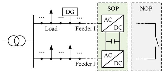
Figure 1.
Installation location of SOP.
In Equation (9), and are, respectively, the active power and reactive power of the VSC connected to node i in time period t. and are, respectively, the active power and reactive power of the VSC connected to node j in time period t. represents the power loss generated when the SOP connecting nodes i and j transmits power. is the loss coefficient of the SOP. is the loss coefficient of the SOP. is the set of flexible interconnection branches. is the set of distribution network nodes.
3.1.2. Mathematical Model of CBs
In Equation (10), is the number of units connected to CBs in period t. is the capacity of each capacitor bank. is the total installed
capacity of CBs.
3.1.3. Mathematical Model of OLTC
The simple mathematical model of OLTC is as follows [38]:
In Equation (11), is the voltage amplitude of node i at period t. is the voltage transformation ratio of the OLTC at period t. is the initial voltage transformation ratio. is the increment per unit transformation ratio. is the adjustment
gear of the OLTC in period t.
3.2. Objective Function
The following two objective functions are established to optimize the operation of the flexibly interconnected distribution network, so as to improve the economy and stability of the system simultaneously.
3.2.1. Minimize Operating Costs
The operation cost consists of two parts: the line loss cost and the switch loss cost. The objective function is as follows:
The system operation cost consists of two parts: the line loss cost and the switch loss cost. Line loss cost consists of the transmission network loss cost and the operating cost of SOPs. Switch loss cost is composed of the operating costs of OLTC and CBs. The objective function is as follows:
In Equation (12), represents the line loss. is the unit cost of line losses. is the resistance between node i and node j. represents the current flowing through the during period t. is the ensemble of the original branches of the distribution network. and are the unit costs
of switch losses for OLTC and CBs, respectively.
3.2.2. Minimize Voltage Deviation
The degree of voltage deviation can be expressed by the sum of the deviations between each node voltage and the rated voltage, which can be expressed as
In Equation (13), represents the rated voltage. represents the number of nodes in the distribution network. and are the upper and lower limits of the desired range of voltage magnitude, respectively. When the voltage amplitude of is within the expected range, the deviation between the voltage during period t and the rated value is not included in .
3.3. Constraint Conditions
The Distflow branch model is used to constrain the power flow of the distribution network [39]. The Distflow branch model is shown in Figure 2 and equations of the Distflow branch model are as follows:
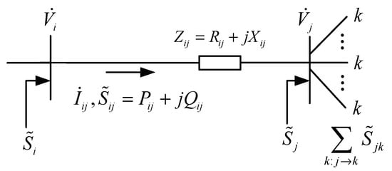
Figure 2.
Distflow branch model.
In Equation (14), represents the complex power injected from node i to node j during period t. represents the complex power injected from node j to node k during period t.
To facilitate the computation of solver, the quadratic form is used to define the voltage constraints. The safety constraints are as follows:
In Equation (15), is the square of the voltage during period t. and are the upper and lower limits of , respectively.
The SOP constraints
are as follows:
In Equation (16), represents the
capacity of the SOP connected between nodes i and j.
The energy balance constraint is as follows:
In Equation (17), is the power injected into the distribution network by the main grid during period t. is the load connected to node i. and are the output of the photovoltaic and wind turbine during period t, respectively.
The constraints of OLTC and CBs are as follows:
In Equations (18) and (19), and are, respectively, the upper limits of the number of operations of OLTC and CBs within one day. is the maximum tap position to which the OLTC can be adjusted. is the maximum
number of capacitor banks that can be connected.
4. Solution Algorithm for the Optimization Model
4.1. Solution to Single-Objective Optimization
The optimization problem in this paper is a non-convex problem. However, the commonly used solvers can only solve convex problems. Therefore, it is necessary to transform the initial model into a mixed-integer second-order cone programming (MISOCP) model through linearization and second-order cone relaxation processes.
4.1.1. Second-Order Cone Relaxation
Relax the phase angles of the nonlinear terms and in the power flow constraints. Let and , so that only the magnitudes of the variables affect the optimization problem, while changes in phase angles do not impact the optimization results. Let , the second-order
cone constraint is finally obtained as
4.1.2. Linearization
There are absolute value terms in the mathematical model of SOP and the objective function F2. Introduce an auxiliary variable to represent the absolute value variable . It is worth noting that only when is less than or greater than will be included in the calculation of the objective function F2. This condition is reflected in the linearization process below. Introduce two auxiliary variables and to represent the absolute value variables and . After linearizing Equations (9) and (13), the following equations can, respectively, be obtained:
is defined in the above text and thus update the mathematical model of OLTC. The tap position selection of OLTC is . A binary variable is introduced to represent the tap position selection situation of the OLTC connecting nodes i and j during period t. If = 1, then the tap position of the OLTC is k during period t. There are absolute value terms in the constraints of OLTC and CBs. In the OLTC model, the change amount of the tap action in every two adjacent periods is divided into a positive change amount and a negative change amount . is replaced by , and thus the updated mathematical model and
constraints of OLTC are, respectively, obtained as follows:
Similarly, the updated constraints for CBs are
obtained as follows [25]:
In Equation (25), and represent the positive and negative changes in the
number of switched capacitor banks in every two adjacent periods, respectively.
4.2. Solution to Multi-Objective Optimization
4.2.1. Multi-Objective Solution Based on the NNC Algorithm
The multi-objective optimization model for the double-layer siting and sizing of the flexible interconnected distribution network constructed in this paper can be summarized as follows:
In Equation (26), and represent the z-th equality
constraint and inequality constraint, respectively. x represents the
decision variable in the control model.
Solve the single-objective problem for the objective function . The obtained value of is its optimal solution and the obtained value of is its worst-case solution . Solve the single-objective problem for the objective function . The obtained value of is its worst-case solution and the obtained value of is its optimal solution . Define as the main objective function and as the secondary objective function. Define the number of Pareto solution sets as . The range of the second objective function and the adjustment step size can be expressed as
The multi-objective optimization model is transformed into the form shown in Equation (28). l is taken different values to continuously adjust the step size of each segment and record the solution result
each time.
In Equation (28), is a very small constant; is a slack variable that is always positive.
4.2.2. Solution Set Screening Based on EW-TOPSIS
The EW-TOPSIS is adopted to screen the multi-objective solution set [40,41]. In this paper, all objective functions are cost-type indicators. The data in the solution set are normalized as follows:
In Equation (30), is the value of the b-th objective function for the a-th solution. and are the normalized objective function values and information entropy, respectively. The element of the decision matrix after obtaining the
normalized original data is as follows:
Calculate the Euclidean distances and between each decision-making alternative and the positive and negative ideal solutions, respectively. The relative closeness of solution a is obtained, which can be expressed as follows. The solution corresponding to the maximum value of is the optimal solution.
The overall research process of this paper is shown in Figure 3.
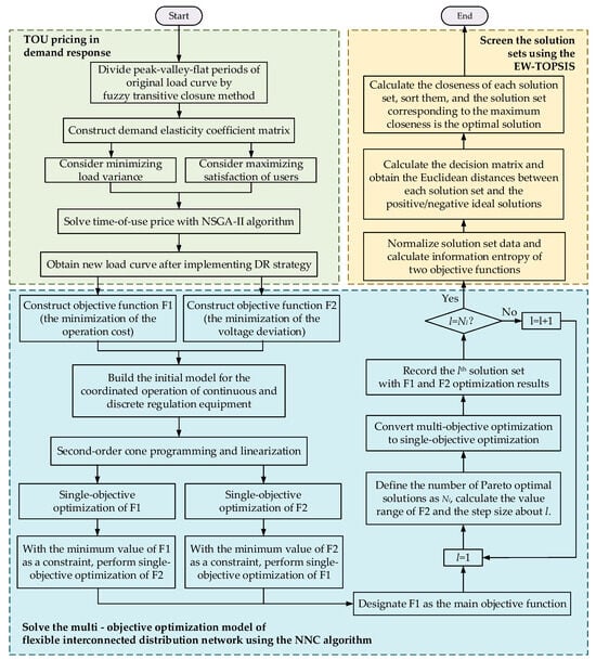
Figure 3.
Research flow chart.
5. Results
5.1. Basic Data
The case simulation in this paper is carried out in MATLAB 2023b. In a 64-bit Windows environment, the Gurobi solver and YALMIP toolbox are used to solve the optimization model. The classical IEEE 33-node distribution system is taken as an example for validity analysis. The structure of the IEEE 33-bus system is shown in Figure 4, with rated voltage of 12.66 kV. The numbers 1 to 33 in Figure 4 represent node serial numbers. The allowable fluctuation range of the per-unit voltage at each node is [0.95, 1.05]. Wind turbine (WT) is connected to nodes 27 and 30, and photovoltaic (PV) is connected to nodes 7, 16, and 17. An OLTC is connected between nodes 1 and 2, and CBs are connected to node 33; the maximum number of operations allowed for both within a day is 4 times. Each capacitor bank has a capacity of 0.5 MW. SOPs are connected between node s 25 and 29, and between node s 12 and 22, respectively, with a capacity of 5 MW and a loss coefficient of 0.02. The unit cost of line loss is 0.08 $/kWh, and the unit costs of switching losses for OLTC and CBs are 1.4 $/time and 0.24 $/time, respectively [21].
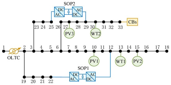
Figure 4.
Structure diagram of IEEE 33-node power distribution system.
5.2. Optimization Results
5.2.1. Implementation Effect of DR Strategy
Based on historical load data, fuzzy clustering is performed on the electrical load curve to divide it into three periods: peak, valley, and flat. The clustering results are shown in Figure 5.
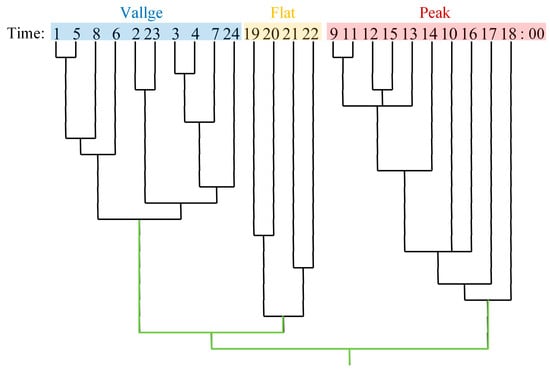
Figure 5.
Clustering division results of peak, flat, and valley periods.
The elasticity coefficient matrix is shown in Table 1. The TOU electricity price is solved using NSGA-II with the objective functions of minimizing the load variance and maximizing the comprehensive satisfaction of users after implementing DR. Among them, the electricity price before the implementation of the DR strategy is 0.11 USD/kWh [42]. The weight of users’ satisfaction with the change in electricity consumption and the weight of their satisfaction with electricity expenses are both 0.5. The population size is set to 250. The maximum number of genetic generations is set to 900. It can be seen from Figure 3 that the clustering results of peak, valley and flat periods. The clustering results of peak, valley and flat periods and the corresponding time-of-use electricity prices are shown in Table 2.

Table 1.
The elasticity coefficient matrix.
Table 2.
Period clustering results and corresponding electricity prices.
The comparison between the load curve after implementing the DR strategy and that before implementation is shown in Figure 6. Compared with the original load curve, after the implementation of DR, the load increases during the flat and valley periods, i.e., 01:00–08:00 and 19:00–24:00; while during the peak period, i.e., 09:00–18:00, the load decreases. After the implementation of the DR strategy, the variance of load has decreased by 23.35%, which proves the effectiveness of the DR strategy in peak shaving and valley filling.
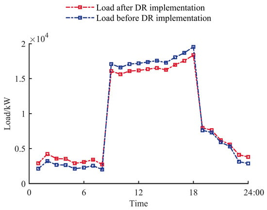
Figure 6.
Comparison of load before and after the implementation of the DR strategy.
5.2.2. Analysis of Optimization Results
The output of WT and PV is shown in Figure 7. The number of Pareto solution sets is set to 20. The NNC algorithm is used to solve the multi-objective operation optimization problem, and the EW-TOPSIS is used to sort and screen the Pareto solution sets according to their closeness. The sorted Pareto solution sets are shown in Figure 8, where the abscissa is the daily operation cost and the ordinate is the daily voltage deviation index. The color scale on the right side of Figure 8 represents the closeness of the schemes to the ideal point. The closer the color of a scheme is to blue, the lower its closeness to the ideal solution; the closer the color is to yellow, the higher its closeness to the ideal solution, that is, the more ideal the scheme is. The scheme with the highest closeness has been marked with a red circle in Figure 8.
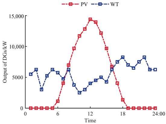
Figure 7.
Output of PV and WT.
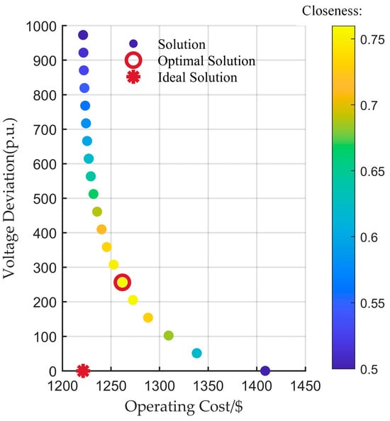
Figure 8.
Pareto solution sets based on the NNC algorithm and solution sets screening based on the EW-TOPSIS.
The optimized active power transmission of the SOP is shown in Figure 9, where the power flowing into the SOP is defined as positive. The active power transmission of the SOP matches the load of the distribution network and the power generated by renewable energy. Since more DGs are connected to the feeders where Node 12 and Node 29 are located, while no DGs are connected to the feeders where Node 22 and Node 25 are located, the power flow of the SOP throughout the day is basically reflected as flowing from Node 12 to Node 22 and from Node 29 to Node 25. From 23:00 to 05:00 the next day, only WT generates power, and there is no PV output. The active power transmission trends of the two SOPs are similar. Due to the small load fluctuation during this period, the change trend of the transmission power of the SOP is similar to that of the WT output.
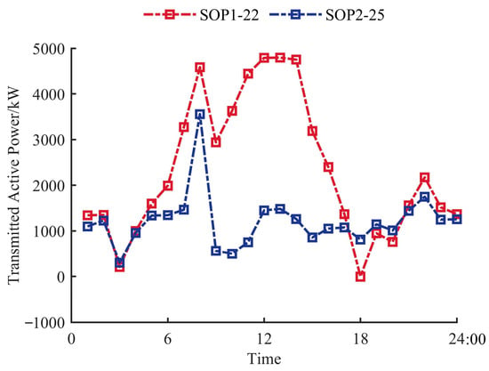
Figure 9.
Active power transmitted by SOPs.
From 06:00 to 08:00, the load is relatively small, with an average of only about 3071 kW. During this period, the output power of DGs increased by 92.36%, equivalent to 6350 kW. Therefore, the transmission powers of SOP1 and SOP2 increased by approximately 2597 kW and 2212 kW, respectively, during this period. During this period, the increase in output of DGs is mainly due to the increase in PV output. The growth in PV output power accounts for 92.12% of the total growth in DG output power. Since more PVs are connected to the feeder where Node 12 is located than to that where Node 29 is located, the increase amplitude of active power transmitted by SOP1 is larger than that by SOP2. From 08:00 to 09:00, the load increased sharply from 2737 kW to 16072 kW, representing a rise of approximately 487.21%. During this period, the PV generation power increased by 2700 kW, while the WT generation power decreased by 2500 kW. The increment of the total generation power of DGs is far less than that of the load and thus insufficient to meet the high load demand, leading to a decrease in the transmission power of SOPs. In the case of a sudden load surge, when the PV output increases and the WT output decreases, the transmission power of SOP1, whose feeder relates to more PVs, is higher than that of SOP2. From 09:00 to 13:00, the load was relatively stable, while the output power of DGs increased by 5025 kW. Therefore, during this period, the active power transmitted by SOPs increased: the output power of SOP1 increased by 1858 kW, and that of SOP2 increased by 939 kW. From 13:00 to 18:00, the load increased by 2011 kW. During this period, the PV output decreased by 12600 kW, while the WT output power only increased by 3750 kW, resulting in a drop in the generation power of DGs. Consequently, the active power transmitted by the two SOPs also decreased. Specifically, the transmission power of SOP2 decreased by 673 kW, while that of SOP1 dropped more significantly, reaching 4799 kW. This is because the feeder connected to SOP1 has a larger number of PV installations than the one connected to SOP2. From 18:00 to 19:00, the PV output power dropped to 0, and the WT output power decreased by 1250 kW. During this period, the load fell sharply by 10,406 kW. Therefore, the transmission power of the two SOPs both increased. From 19:00 to 22:00, the average output power of WT was 7312 kW, while the average load stood at 6837 kW. Therefore, the transmission power of the two SOPs mainly showed an upward trend. The optimized reactive power transmission of the SOPs is shown in Figure 10. The reactive power transmission of the SOPs changes with the change of user electrical load, and the two trends are basically consistent.
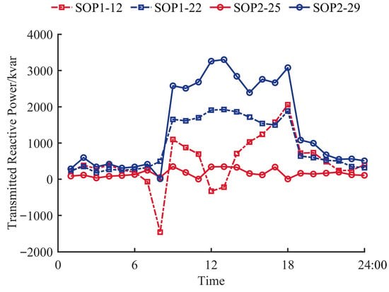
Figure 10.
Reactive power transmitted by SOPs.
The per-unit values of voltages at each node in the distribution network throughout the day are shown in Figure 11. Among the data of 24 time periods for the 33-node system, the maximum value of the voltage per unit is 1.05, and the minimum value is 0.95. A total of 96% of the per-unit values of voltages are within the range of [0.96 p.u., 1.04 p.u.], which meets the requirements for safe and reliable operation of the system, thus proving the effectiveness of the method proposed in this paper.
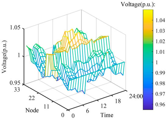
Figure 11.
The per-unit values of voltages at each node throughout the day.
5.3. Comparison Between Multi-Objective and Single-Objective Optimization
The multi-objective optimization results are compared with the single-objective optimization results, and the comparison results are shown in Table 3. Compared with the single-objective optimization that only considers minimizing the operation cost, the multi-objective optimization that comprehensively considers minimizing the operation cost and minimizing the voltage deviation reduces the voltage deviation by 34.32%, while the operation cost only increases by 3.17%. Compared with the single-objective optimization that only considers minimizing the voltage deviation, the multi-objective optimization reduces the operation cost by 17.94%, while the voltage deviation only increases by 11.30%. This paper realizes the trade-off between the two conflicting indicators of voltage deviation degree and operation cost through multi-objective optimization. The comparison between the results of multi-objective and single-objective optimization proves the effectiveness of the multi-objective optimization method proposed.
Table 3.
Comparison results between multi-objective and single-objective optimization.
5.4. Comparison of Optimization Results Under Different Scheme
To verify the effectiveness of the proposed method, two additional schemes are put forward for comparative analysis with the scheme proposed in this paper. The specific schemes are as follows:
- Scheme 1: After implementing the DR strategy, the SOP operates in coordination with CBs and OLTC, which is the scheme proposed in this paper.
- Scheme 2: Without implementing the DR strategy, the SOP operates in coordination with CBs and OLTC.
- Scheme 3: After implementing the DR strategy, only the operation of CBs and OLTC is considered.
The daily operation cost of the distribution network under the three schemes is shown in Figure 12. The daily voltage of Node 12 in the distribution network under the three schemes is shown in Figure 13. In the case where SOPs are connected to operate in coordination with traditional control equipment, Scheme 2 only considers the optimization of the load supply side without taking into account the optimization of the load demand side. Therefore, compared with Scheme 1, the load fluctuation in Scheme 2 is greater, resulting in higher operation cost in Scheme 2. The voltage fluctuation trend and amplitude of Node 12 in Scheme 1 and Scheme 2 are similar.
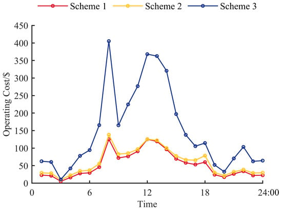
Figure 12.
Comparison of daily operating costs among the three schemes.
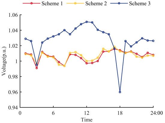
Figure 13.
Comparison of Node 12 voltage within one day among the three schemes.
In the case where both the load supply and demand sides are optimized, the operation cost of Scheme 3 is higher than that of Scheme 1 in each time period. Especially when the DG output is large, the operation cost of Scheme 3 is much higher than that of Scheme 1. In addition, the voltage of Scheme 3 is greatly affected by the fluctuation of DG output. From 18:00 to 19:00, the load is large while the DG output is small, and the voltage of Scheme 3 drops significantly. From 11:00 to 14:00, the DG output is higher than the load demand, and the voltage of Scheme 3 increases significantly, with voltage over-limit occurring from 12:00 to 14:00. It can be proved that the SOP can alleviate the problem of increased operation costs caused by DG integration.
The daily operation cost and average node voltage deviation of the distribution network of the three schemes are shown in Table 4. Compared with the scheme proposed in this paper, the non-implementation of the DR strategy results in an increase in operation cost by 13.83% and an increase in voltage deviation by 4.14%. Compared with the scheme proposed in this paper, the non-integration of SOPs leads to an increase in operation cost by 182.40% and an increase in voltage deviation by 113.02%.
Table 4.
Comparison of results of the three schemes.
5.5. Model Validation Based on Alternative Parameters
The peak-shaving and valley-filling effect of the alternative load according to the strategy proposed in this paper is illustrated in Figure 14. With the proposed TOU pricing strategy, the load variance has decreased by 25.27%. Based on the alternative data of DG output shown in Figure 15, the multi-objective Pareto solution set is obtained, as shown in Figure 16. The scheme selected based on EW-TOPSIS is marked with red circles in Figure 16. Among the voltage values of 33 nodes during 24 periods, a 96.84% fall within the range of [0.96, 1.04].
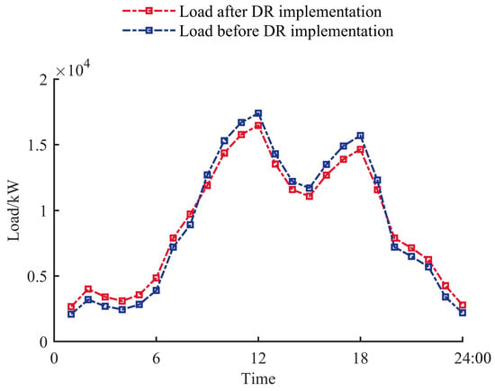
Figure 14.
Comparison of alternative load before and after the implementation of the DR strategy.
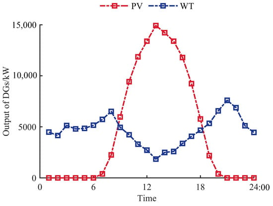
Figure 15.
Alternative data of wind and photovoltaic power generation.
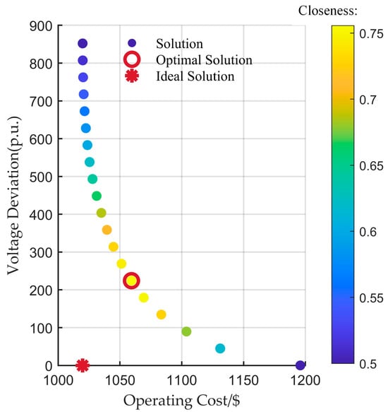
Figure 16.
Pareto solution sets and their screening based on the alternative data.
The daily operation cost and average node voltage deviation of the three schemes based on the alternative parameters are shown in Table 5. Comparing Scheme 1 with the scheme proposed in this paper, Scheme 2 with non-implementation of the DR strategy results in an increase in operation cost by 10.16% and an increase in voltage deviation by 3.75%. Comparing Scheme 1 with the scheme proposed in this paper, Scheme 3 with the non-integration of SOPs leads to an increase in operation cost by 113.77% and an increase in voltage deviation by 63.75%.
Table 5.
Comparison of results of the three schemes based on the alternative parameters.
5.6. Research Limitations and Applicable Scenarios
In this paper, the daily load is divided into three time periods, which are peak, flat, and valley. It is only applicable to the specific load curve in the paper and lacks universality. Regions with high load density require refinement into five time periods, which are critical peak, peak, flat, valley, and deep valley, while regions with mild load fluctuations only need two time periods, which are peak and valley. Meanwhile, the peak shaving and valley filling based on the TOU pricing strategy must be implemented in regions dominated by transferable loads as a prerequisite, and it is difficult to achieve results in regions where rigid loads are predominant. Although the main influencing factors have been incorporated into the mathematical modeling of devices, some actual operational constraints such as heat accumulation constraint of CBs and response time constraint of OLTC have not been fully considered for the sake of model simplification. The model will be further refined in future studies.
If the power supply from distributed generators (DGs) on one feeder is far greater than the feeder’s load demand, while the power supply from DGs on another feeder is insufficient to meet its load demand, the soft open point (SOP) can be used to achieve flexible interconnection between the two feeders. This helps improve the economy and stability of the distribution network. In addition, the collaborative optimization model relies on the characteristics of radial networks and cannot be directly applied to multi-ring network structures.
6. Conclusions
To address the issues of voltage instability and increased network loss caused by load and DG output fluctuations in ADNs, as well as the challenge of delayed response from traditional control equipment, this paper proposes a multi-objective operation optimization method for the collaboration between traditional control equipment and SOPs based on the DR strategy. TOU price periods are divided using the fuzzy transitive closure method, and TOU prices are formulated in combination with the NSGA-II algorithm. The NNC algorithm and EW-TOPSIS are employed to solve and screen the multi-objective optimization model for collaborative operation. The advantages of the strategy with collaborative optimization of both load supply and demand sides proposed in this paper are as follows: (1) it achieves peak shaving and valley filling of loads through DR strategy; (2) it combines the continuous equipment SOP with discrete traditional equipment for regulation, improving the accuracy of power flow and voltage control; (3) multi-objective optimization realizes the optimal trade-off between operation cost and voltage stability. Based on two sets of load data and DG output data, simulation verification is conducted using the IEEE 33-bus system as an example. The results show that the DR strategy can significantly improve the load distribution, with the load variance based on two sets of experimental data reduced by 23.35% and 25.27%, respectively; compared with single-objective optimization, multi-objective optimization reduces voltage deviation by 34.32% while increasing operation cost by only 3.17%; and both the integration of SOPs and the implementation of the DR strategy can effectively enhance the economic efficiency and stability of system operation.
Author Contributions
Conceptualization, Y.Y. and Z.W.; methodology, Y.Y.; software, Z.W.; validation, Y.Y., Z.W. and T.Y.; formal analysis, T.Y.; investigation, Z.W.; resources, T.Y. and Z.Y.; data curation, Z.Y. and H.X.; writing—original draft preparation, Z.W.; writing—review and editing, Z.Y. and Y.Y.; visualization, H.X.; supervision, F.R.; project administration, F.R.; funding acquisition, Y.Y. All authors have read and agreed to the published version of the manuscript.
Funding
This research was funded by research on Key Technologies and Equipment of Flexible interconnected System Based on Grid-forming Control of Science and Technology Project of China Southern Power Grid Company, project number GDKJXM20240114 (032000KC24010005).
Data Availability Statement
The original contributions presented in this study are included in the article. Further inquiries can be directed to the corresponding author.
Conflicts of Interest
Author Yinzhou Yao, Ting Yang, Haoting Xu was employed by the Zhongshan Power Supply Bureau of Guangdong Power Grid Co., Ltd. The remaining authors declare that the research was conducted in the absence of any commercial or financial relationships that could be construed as a potential conflict of interest.
Abbreviations
The following abbreviations are used in this manuscript:
| AND | active distribution networks |
| CB | capacitor bank |
| DG | distributed generation |
| DR | demand response |
| EW-TOPSIS | Entropy Weight and Technique for Order Preference by Similarity to an Ideal Solution |
| MISCCP | mixed-integer second-order cone programming |
| NNC | normalized normal constraint |
| NSGA | nondominated sorting genetic algorithm |
| OLTC | on-load tap changer |
| PV | photovoltaic |
| SOP | soft open point |
| TOU | time-of-use |
| WT | wind turbine |
References
- Sun, J.B.; Wang, Y.; He, Y.; Cui, W.R.; Chao, Q.C.; Shan, B.G.; Wang, Z.; Yang, X.F. The energy security risk assessment of inefficient wind and solar resources under carbon neutrality in China. Appl. Energy 2024, 360, 122889. [Google Scholar] [CrossRef]
- Ge, Z.Z.; Xu, Z.Z.; Li, J.; Xu, J.; Xie, J.B.; Yang, F.B. Technical-economic evaluation of various photovoltaic tracking systems considering carbon emission trading. Sol. Energy 2024, 271, 112451. [Google Scholar] [CrossRef]
- Shi, Q.L.; Yang, P.; Tang, B.; Lin, J.T.; Yu, G.Z.; Muyeen, S.M. Active distribution network type identification method of high proportion new energy power system based on source-load matching. Int. J. Electr. Power Energy Syst. 2023, 153, 109411. [Google Scholar] [CrossRef]
- Yu, N.P.; Zhang, S.R.; Qin, J.T.; Hidalgo-Gonzalez, P.; Dobbe, R.; Liu, Y.; Dubey, A.; Wang, Y.B.; Dirkman, J.; Zhong, H.W.; et al. Data-driven control, optimization, and decision-making in active power distribution networks. Appl. Energy 2025, 397, 126253. [Google Scholar] [CrossRef]
- Amako, E.A.; Arzani, A.; Mahajan, S.M. Heuristic-Based Scheduling of BESS for Multi-Community Large-Scale Active Distribution Network. Electricity 2025, 6, 36. [Google Scholar] [CrossRef]
- Lu, Z.; Li, Z.; Guo, X.; Yang, B. Optimal Planning of Hybrid Electricity–Hydrogen Energy Storage System Considering Demand Response. Processes 2023, 11, 852. [Google Scholar] [CrossRef]
- Wang, G.; Qian, Z.; Feng, X.; Ren, H.; Zhou, W.; Wang, J.; Ji, H.; Li, P. Data-Driven Operation of Flexible Distribution Networks with Charging Loads. Processes 2023, 11, 1592. [Google Scholar] [CrossRef]
- Arévalo, P.; Benavides, D.; Tostado-Véliz, M.; Aguado, J.A.; Jurado, F. Smart monitoring method for photovoltaic systems and failure control based on power smoothing techniques. Renew. Energy 2023, 205, 366–383. [Google Scholar] [CrossRef]
- Agalgaonkar, Y.P.; Pal, B.C.; Jabr, R.A. Distribution voltage control considering the impact of PV generation on tap changers and autonomous regulators. IEEE Trans. Power Syst. 2014, 29, 182–192. [Google Scholar] [CrossRef]
- Wang, S.; Dong, Z.Y.; Chen, C.; Fan, H.; Luo, F. Expansion Planning of Active Distribution Networks with Multiple Distributed Energy Resources and EV Sharing System. IEEE Trans. Smart Grid 2020, 11, 602–611. [Google Scholar] [CrossRef]
- Ruan, H.; Gao, H.; Liu, Y.; Wang, L.; Liu, J. Distributed Voltage Control in Active Distribution Network Considering Renewable Energy: A Novel Network Partitioning Method. IEEE Trans. Power Syst. 2020, 35, 4220–4231. [Google Scholar] [CrossRef]
- Ji, H.R.; Wang, C.S.; Li, P.; Zhao, J.L.; Song, G.Y.; Ding, F.; Wu, J.Z. A centralized-based method to determine the local voltage control strategies of distributed generator operation in active distribution networks. Appl. Energy 2018, 228, 2024–2036. [Google Scholar] [CrossRef]
- Huo, Y.D.; Li, P.; Ji, H.R.; Yan, J.; Song, G.; Wu, J.; Wang, C. Data-driven adaptive operation of soft open points in active distribution networks. IEEE Trans. Ind. Inform. 2021, 17, 8230–8242. [Google Scholar] [CrossRef]
- Zhang, J.R.; Foley, A.; Wang, S.Y. Optimal planning of a soft open point in a distribution network subject to typhoons. Int. J. Electr. Power Energy Syst. 2021, 129, 106839. [Google Scholar] [CrossRef]
- Zhang, J.X.; Wang, B.; Ma, H.R.; He, Y.F.; Wang, Y.W.; Xue, Z.C. Reliability Evaluation of Cabled Active Distribution Network Considering Multiple Devices—A Generalized MILP Model. Processes 2023, 11, 3404. [Google Scholar] [CrossRef]
- Jiang, X.; Zhou, Y.; Ming, W.; Yang, P.; Wu, J. An Overview of Soft Open Points in Electricity Distribution Networks. IEEE Trans. Smart Grid 2022, 13, 1899–1910. [Google Scholar] [CrossRef]
- Wang, J.; Wang, W.; Yuan, Z. Operation Optimization Adapting to Active Distribution Networks Under Three-Phase Unbalanced Conditions: Parametric Linear Relaxation Programming. IEEE Syst. J. 2023, 17, 4324–4335. [Google Scholar] [CrossRef]
- Chen, L.; Zhang, N.; Yang, X.F.; Pei, W.; Zhao, Z.X.; Zhu, Y.N.; Xiao, H. Synergetic optimization operation method for distribution network based on SOP and PV. Glob. Energy Interconnect. 2024, 7, 130–141. [Google Scholar] [CrossRef]
- Zhang, Y.; Li, D.; Gan, J.; Ren, Q.; Yu, H.; Zhao, Y.; Zhang, H. A Cooperative Operation Optimization Method for Medium- and Low-Voltage Distribution Networks Considering Flexible Interconnected Distribution Substation Areas. Processes 2025, 13, 1123. [Google Scholar] [CrossRef]
- Ji, H.R.; Wang, C.S.; Li, P.; Zhao, J.; Song, G.; Wu, J. Quantified flexibility evaluation of soft open points to improve distributed generator penetration in active distribution networks based on difference-of-convex programming. Appl. Energy 2018, 218, 338–348. [Google Scholar] [CrossRef]
- Li, P.; Ji, H.R.; Wang, C.S.; Zhao, J.; Song, G.; Ding, F.; Wu, J. Coordinated control method of voltage and reactive power for active distribution networks based on soft open point. IEEE Trans. Sustain. Energy 2017, 8, 1430–1442. [Google Scholar] [CrossRef]
- Zhang, J.; Wang, T.; Liao, Z.; Tang, Z.; Wang, H.; Yue, J.; Shu, J.; Dong, Z. Flexible interconnection strategy for distribution networks considering multiple soft open points siting and sizing. Electr. Power Syst. Res. 2025, 241, 111335. [Google Scholar] [CrossRef]
- Zhang, J.; Wang, T.; Liao, Z.; Tang, Z.; Pei, Y.; Cui, Q.; Shu, J.; Zheng, W. Optimal operation strategy for distribution network with high-penetration distributed PV based on soft open point and multi-device collaboration. Energy 2025, 325, 136191. [Google Scholar] [CrossRef]
- Zheng, H.K.; Shi, T.J. Bi-level optimization of distribution network based on soft open point and reactive power compensation device. Autom. Electr. Power Syst. 2019, 43, 117–123. [Google Scholar]
- Xiong, M.; Yang, X.; Zhang, Y.; Wu, H.; Lin, Y.; Wang, G. Reactive power optimization in active distribution systems with soft open points based on deep reinforcement learning. Int. J. Electr. Power Energy Syst. 2024, 155 Pt B, 109601. [Google Scholar] [CrossRef]
- Yong, C.S.; Kong, X.Y.; Chen, Y.; E, Z.J.; Cui, K.; Wang, X. Multiobjective Scheduling of an Active Distribution Network Based on Coordinated Optimization of Source Network Load. Appl. Sci 2018, 8, 1888. [Google Scholar] [CrossRef]
- Xu, X.M.; Niu, D.X.; Peng, L.Y.; Zheng, S.P.; Qiu, J.P. Hierarchical multi-objective optimal planning model of active distribution network considering distributed generation and demand-side response. Sustain. Energy Technol. Assess. 2022, 53, 102438. [Google Scholar] [CrossRef]
- Menghwar, M.; Yan, J.; Chi, Y.N.; Amin, M.A.; Liu, Y.Q. A market-based real-time algorithm for congestion alleviation incorporating EV demand response in active distribution networks. Appl. Energy 2024, 356, 122426. [Google Scholar] [CrossRef]
- Chen, Q.; Wang, W.Q.; Wang, H.Y.; Dong, Y.C.; He, S. Information gap-based coordination scheme for active distribution network considering charging/discharging optimization for electric vehicles and demand response. Int. J. Electr. Power Energy Syst. 2023, 145, 108652. [Google Scholar] [CrossRef]
- Zhang, N.; Chen, J.; Liu, B.; Ji, X. Optimized Scheduling of Integrated Energy Systems with Integrated Demand Response and Liquid Carbon Dioxide Storage. Processes 2024, 12, 292. [Google Scholar] [CrossRef]
- Xue, W.; Zhao, X.; Li, Y.; Mu, Y.; Tan, H.; Jia, Y.; Wang, X.; Zhao, H.; Zhao, Y. Research on the Optimal Design of Seasonal Time-of-Use Tariff Based on the Price Elasticity of Electricity Demand. Energies 2023, 16, 1625. [Google Scholar] [CrossRef]
- Kong, Q.; Fu, Q.; Lin, T.; Zhang, Y.; Peng, Z.; Wan, Y.; Guo, L. Optimal peak-valley time-of-use power price model based on cost-benefit analysis. Power Syst. Prot. Control 2018, 46, 60–67. [Google Scholar]
- Huang, J.; Chen, H.; Zhong, J.; Chen, W.; Duan, S.; Zheng, X. Optimal Time-of-Use Price Strategy with Selecting Customer’s Range Based on Cost. Electr. Power 2020, 53, 107–116. [Google Scholar]
- Zhang, Z.H.; Lei, D.Y.; Jiang, C.H.; Luo, J.; Xu, Y.; Li, J. A bi-level planning model and its solution method of AC/DC hybrid distribution network based on second-order cone programming and NNC method. Proc. CSEE 2023, 43, 70–85. [Google Scholar]
- Hashemi, S.M.; Arasteh, H.; Shafiekhani, M.; Kia, M.; Guerrero, J. Multi-objective operation of microgrids based on electrical and thermal flexibility metrics using the NNC and IGDT methods. Int. J. Electr. Power Energy Syst. 2023, 144, 108617. [Google Scholar] [CrossRef]
- Arasteh, H.; Kia, M.; Vahidinasab, V.; Shafie-Khah, M.; Catalão, J.P. Multiobjective generation and transmission expansion planning of renewable dominated power systems using stochastic normalized normal constraint. Int. J. Electr. Power Energy Syst. 2020, 121, 106098. [Google Scholar] [CrossRef]
- Fan, Z.; Wan, Z.; Gao, L.; Xiong, Y.; Song, G. A Multi-Objective Optimal Configuration Method for Microgrids Considering Zero-Carbon Operation. IEEE Access 2023, 11, 87366–87379. [Google Scholar] [CrossRef]
- Yang, X.D.; Jiang, W.T.; Ma, J.; Xu, D.; Zhang, C.J.; Yang, Y.; Xu, Z.C. Flexibility provision by virtual power line and soft open point in AC/DC distribution systems. Int. J. Electr. Power Energy Syst. 2025, 166, 110528. [Google Scholar] [CrossRef]
- Huang, M.Y.; Zhang, Q.P.; Zhang, S.X.; Yan, Z.; Gao, B.; Li, X. Distribution network reconfiguration considering demand-side response with high penetration of clean energy. Power Syst. Prot. Control 2022, 50, 116–123. [Google Scholar]
- Ji, W.; Lan, L.; Shen, L.; Shi, D.; Wang, C. Dynamic Identification Method of Distribution Network Weak Links Considering Disaster Emergency Scheduling. Energies 2025, 18, 3519. [Google Scholar] [CrossRef]
- Shao, C.; Wei, B.; Liu, W.; Yang, Y.; Zhao, Y.; Wu, Z. Multi-Dimensional Value Evaluation of Energy Storage Systems in New Power System Based on Multi-Criteria Decision-Making. Processes 2023, 11, 1565. [Google Scholar] [CrossRef]
- Li, P.; Wu, D.F.; Li, Y.W.; Liu, H.; Wang, N.; Zhou, X. Optimal Dispatch of Multi-microgrids Integrated Energy System Based on Integrated Demand Response and Stackelberg game. Proc. CSEE 2021, 41, 1307–1321+1538. [Google Scholar]
Disclaimer/Publisher’s Note: The statements, opinions and data contained in all publications are solely those of the individual author(s) and contributor(s) and not of MDPI and/or the editor(s). MDPI and/or the editor(s) disclaim responsibility for any injury to people or property resulting from any ideas, methods, instructions or products referred to in the content. |
© 2025 by the authors. Licensee MDPI, Basel, Switzerland. This article is an open access article distributed under the terms and conditions of the Creative Commons Attribution (CC BY) license (https://creativecommons.org/licenses/by/4.0/).