Performance, Fragility and Robustness for a Class of Quasi-Polynomials of Degree Two

Abstract

In recent years the use of delayed controllers has increased considerably, since they can attenuate noise, replace derivative actions, avoid the construction of observers, and reduce the use of extra sensors, while maintaining inherent insensitivity to high-frequency noise. Therefore, it is important to continue improving the tuning of these controllers, including properties such as performance, fragility and robustness that may be beneficial for this purpose. However, currently most studies prioritize tuning using only the performance property, some others only the fragility property, and some less only the robustness property. This work provides the first rigorous joint analysis of performance, fragility, and robustness for a class of systems whose characteristic equation is a quasi-polynomial of degree two, filling a gap in the current literature. Thus, necessary and sufficient conditions are proposed to improve the tuning of delayed-action controllers by ensuring a exponential decay rate on the convergence of the closed-loop system response (performance) and by ensuring stabilization and/or trajectory tracking in the face of changes in system parameters (robustness) and controllers gains (fragility). To illustrate and corroborate the effectiveness of the proposed theoretical results, a real-time implementation is presented on a mobile prototype consisting of an omnidirectional mobile robot, to streamline/guarantee trajectory tracking in response to variations in controller gains and robot parameters. This implementation and application of theoretical results are possible thanks to the proposal of a novel delayed nonlinear controller and some simple but strategic algebraic manipulations that reduce the original problem to the study of a quasi-polynomial of degree 9 with three commensurable delays. Finally, our results are compared with a classical proportional nonlinear controller showing that our proposal is relevant.

1. Introduction

Robust control theory is a branch of control theory that focuses on a controller’s ability to maintain system stability and performance in the presence of disturbances, and it can be studied from the perspectives of both robust performance and robust stability [1].

The performance robustness of a system refers to its ability to maintain tracking of reference trajectories, even in the presence of load disturbances, changes in the set point, and to reject disturbances in general. On the other hand, robust stability refers to a system’s ability to maintain stability despite disturbances. According to Alfaro [2], the study of robust stability requires the examination of perturbations in both system parameters and controller gains, with the latter being referred to as fragility, therefore, they should be analyzed independently. For the aforementioned reasons, proper tuning of a controller must achieve a satisfactory balance of performance, fragility, and robustness in the face of system parameter disturbances.

It is widely recognized that one of the most used controllers in industry is of the Proportional Integral Derivative (PID) type [3]. There is a specific subclass of controllers within this family that approximates the derivative stage with a time delay to avoid its use. Under certain circumstances, this approach has a stabilizing effect, and the time delay can be used as a control parameter. This topic has been thoroughly studied in [4,5,6,7], among others. In recent years the use of a delayed-action in the controllers has increased significantly, because this type of action is a more efficient alternative to stabilize systems [4,8], it can replace a classic derivative-action [9,10], thus avoiding the use of observers or additional sensors, it usually attenuates noise present in actuators and sensor measurements [11], besides being easy to implement in practical applications [12,13], among others. However, there are currently few criteria for tuning delayed-action controllers. Therefore studies of performance, fragility and robustness of the closed-loop system can help develop criteria that improve delayed-action tuning.

Describing the system performance can be challenging due to the various approaches and characteristics that require evaluation. These can range from analyzing transient response to disturbance rejection. In the field of delayed controllers, the study of the spectral abscissa has gained significant interest in recent years as it represents the dominant roots of the system spectrum. This dominant roots determine the maximum decay that the system can reach, therefore, its knowledge becomes essential. Analyzing the spectral abscissa is related to study of the relative stability of the system, also known as $\sigma$-stability, as $\sigma$ represents the real part of the dominant roots of the system spectrum. Significant progress has been made in this area, in [14] tuning rules for PR controllers are presented, while in [15] the tuning rules for proportional integral delayed controllers for second-order systems are analyzed. For a linear time-invariant delay equation, in [16], conditions for the existence of a pair of complex conjugate dominant roots are presented. An approach to find the gains of a controller that provides the maximum decay rate of the closed-loop response for a LTI time-delay system is presented in [17]. In [18], placement of a fourth order multiple root for a first order system subject to a PID controller is studied: a multiplicity-induced dominancy (MID) strategy is used to design and tune the controller gains to ensure a specified decay rate of the closed-loop response. In [19], it is proven that the minimum value of the spectral of a second order system subject to a delayed state feedback controller is attained at a root of maximal multiplicity. In [20], fragility for several systems subject to a PI controller is studied.

Controller fragility refers to the susceptibility to performance degradation or instability due to variations in the controller gains. The point in the controller gain space that exhibits the highest resilience to controller parameter disturbances is commonly referred to as the least fragile point. This topic has received considerable attention in the delay-free case, but not as much in the delayed case. However, recent significant progress has been made. In [21], an approach that guarantees the maximal robustness with respect to controller gains disturbances is presented. For delay models of TCP/AQM networks, a non-fragile PI controller that admits uncertainties in the network parameters and the controller gains disturbances is provided in [22]. On the other hand, ref. [23] estimates the non-fragility of PI AQM controllers, while [24] presents an approach to analyze and design non-fragile PI controllers using a geometric approach. In [25], a procedure to determine the non-fragility controllers used to stabilize closed-loop systems with a delay is presented. This approach involves identifying the center of the largest circle that can be inscribed in a stability region of the parameter plane of the closed-loop system.

In the context of robustness, one subject that continues to interest the scientific community is determining conditions that ensures the system stability in the face of parametric variations within a set. Frequently this requires a stability analysis of a family of polynomials. Some contributions includes: interval polynomials [26], polytopes of polynomials [27], diamonds of polynomials [28], segments of polynomials [29], and cones of polynomials [30], to mention a few. However, there are few criteria that address this topic for quasi-polynomials and even fewer when the point with the greatest robustness is desired. Among which we can mention: in [31] for uncertain continuous singular systems with state delay and parameter uncertainty, necessary and sufficient conditions for generalized quadratic stability and stabilization are given, while [32] provides sufficient conditions for parameter dependent stability and stabilizability for linear systems with state delays where the parameters of the systems are not completely known. In [33], the robust stability of uncertain quasi-polynomials problem is addressed, where frequency-sweeping conditions for interval, diamond, and spherical quasi-polynomial families are given.

This contribution presents a comprehensive analytical study to jointly evaluate performance, fragility, and robustness for a class of systems whose characteristic equation is a quasi-polynomial of degree two. This study is novel, as no prior research addressing this framework—spanning theoretical derivations, experimental validation, and benchmarking against established techniques in the field—has been reported in the literature. Specifically, we derive necessary and sufficient conditions to enhance the tuning of delayed-action controllers, ensuring performance (an exponential decay rate in the closed-loop system response convergence), robustness (stabilization and/or trajectory tracking under variations in system parameters), and fragility (resilience to perturbations in controller gains). Additionally, the paper presents necessary and sufficient conditions to ensure stability for this class of systems in the presence of parameter and gain variations. To validate and illustrate the theoretical results, we present an implementation on an experimental platform. The platform consists of an omnidirectional mobile robot (OMR) used for trajectory tracking tasks and an advanced optical motion capture system (^©Vicon Motion Systems Ltd, Oxford, UK) as sensor. Here, we experimentally analyze the performance, fragility, and robustness in the face of parametric variations and external disturbances. Links to some videos of the OMR performance are given. Also, a comparison with a classical control is presented, thus showing that our proposal is a more efficient alternative.

The rest of the paper is organized as follows. Section 2 presents problem statement and manuscript’s contribution. Results for determining the $\sigma$-stability regions are given in Section 3. While in Section 4 and Section 5 results are presented to obtain the best performance point and the least fragile point for a delayed controller, respectively. Next, in Section 6 results are also proposed to obtain the greatest robustness point. In addition, in Section 7, results are proposed to try to obtain a balance or correction among performance, fragility and robustness. Finally, to validate all the theoretical results, Section 8 presents the real-time implementation on an OMR and a comparison with a classical controller from the literature. The contribution ends with some concluding remarks in Section 9.

2. Problem Statement and Contribution

2.1. Problem Statement

Suppose that the quasi-polynomial of degree two

$$q(a,k,s)=a_0+a_{1}s+a_2{k}_r{\mathrm{e}}^{-\tau s}$$

(1)

is the characteristic quasi-polynomial of a closed-loop system. Here $a=(a_0,a_1,a_2)\in A\subseteq {\mathbb{R}}^3$, $a_1,a_2\ne 0$ is the set of parameters of the system, $k=(k_r,\tau )\in K\subseteq {\mathbb{R}}^{+}\times {\mathbb{R}}^{+}$ is the set of gains of a time-delay controller, and $s=\sigma \pm i\omega$ is a complex variable with $\omega \in {\mathbb{R}}^{+}$, $\sigma \in {\mathbb{R}}^{-}$ and $i^2=-1$. In this paper we study the following three properties of a system, which we make precise later.

Performance. For a given set of system parameters, this property will be understood as the capacity of a controller gains to enforce a prescribed convergence rate toward a desired reference signal or set-point in the system response. Although determination of a system’s exponential decay rate constitutes a fundamental aspect of this objective, it merely represents one necessary condition within a comprehensive stability and performance analysis framework. We will denote by $k^{\ast ,p}$ the best performance point.

Fragility. Also, for a given set of system parameters, the fragility property consists in determining the capacity of invariance on the stability of a system response due to unexpected changes in the controller’s gains. We will denote by $k^{\ast ,f}$ the least fragile point.

Robustness. Now, for a given set of controller gains, the robustness property consists in determining the capacity of invariance on the stability of the response of a system due to unexpected changes in the process parameters. We will denote by $a^{\ast ,r}$ the greatest robust point.

Despite the seemingly simple form of the quasi-polynomial (1), its comprehensive analysis presents significant challenges. To the best of the authors’ knowledge, no existing studies have simultaneously addressed the tripartite consideration of performance, fragility and robustness properties for delayed-action controller tuning. This research gap is particularly critical as these combined properties are essential for ensuring closed-loop system stability under both parameter variations and gain perturbations. As mentioned in [2], fragility and robustness are very similar properties, which causes confusion and/or equal treatment. However, there are subtle differences between them, reasons why it is recommended to analyze them independently. A clear difference between these two properties is the working plane: while fragility is determined in the $\tau k_r$-plane, robustness is determined in the $a_0{a}_1$-plane, where $(\tau ,k_r)$ are controller gains and $(a_0,a_1)$ are system/plant parameters.

2.2. Contribution

As previously established, time-delay controllers offer distinct advantages over classical controllers, including simplicity of implementation and inherent noise attenuation properties. However, the existing literature reveals a fragmented approach to controller tuning: some studies only focus on performance optimization, others address fragility concerns, with limited attention to robustness considerations. In this contribution we present a unified tuning methodology that simultaneously incorporates all three critical properties. Specifically, for quasi-polynomial (1), we propose the following:

• Given a set of system parameters $a\in A$, necessary and sufficient conditions are proposed to determine the controller gains that provide best performance $(k^{\ast ,p}\in K)$, and the controller gains that provide least fragility ($k^{\ast ,f}\in K$).
• Given a set of controller gains $k\in K$, necessary and sufficient conditions are proposed to determine the system parameters that ensure greatest robustness ($a^{\ast ,r}\in A$).
• Furthermore, if a controller is tuned to the best performance $k=k^{\ast ,p}$, then we propose theoretical results to determine the invariance capability in the stability of the system response to unexpected changes in controller gains (fragility) or system parameters (robustness).
• Similarly, if a controller is tuned with the least fragility $k=k^{\ast ,f}$, and/or the system is adjusted with the parameters of greatest robustness $a=a^{\ast ,r}$, then theoretical results can determine the system’s response performance.
• As an interconnection among the three properties (performance, fragility and robustness), we propose necessary and sufficient conditions to determine the invariance capacity in stabilizing the closed-loop system response in the $\tau k_r{a}_1$-space.
• To illustrate the proposed results, an implementation is carried out on an OMR using a novel delayed nonlinear controller.
• Finally, to demonstrate the efficiency of our proposal, a comparison is made with a conventional controller using traditional techniques.

Next, we define and obtain the workspace that we call $\sigma$-stability regions.

3. $\sigma$-Stability Regions

The following definitions rely on continuity of roots of the quasi-polynomial $q(a,k,s)$ with respect to the parameters a and the gains k, see [34].

Definition 1. 

For a fixed $a\in A$ and $\sigma \le 0$, let ${\mathrm{\Gamma }}_{a,\sigma }$ be the set of all gains $k\in K$ such that at least one root of (1) lies on the vertical line $\mathrm{Re}\left(s\right)=\sigma$, that is,

$${\mathrm{\Gamma }}_{a,\sigma }=\{k\in K:q(a,k,s)=0\mathrm{for}\mathrm{some}s=\sigma +i\omega \}.$$

The curve ${\mathrm{\Gamma }}_{a,\sigma }$ divides K into subregions where the quasi-polynomial (1) has a constant number of complex roots with a real part greater than $\sigma$, namely,

$$K=K_{a,\sigma }^0\cup K_{a,\sigma }^1\cup K_{a,\sigma }^2\cup \cdots ,$$

where

$$\begin{array}{cc}\hfill K_{a,\sigma }^m=\{& k\in K:q(a,k,s)\mathrm{has} \mathrm{exactly} m\mathrm{roots} \mathrm{with} \mathrm{real} \mathrm{part}>\sigma \}.\hfill \end{array}$$

The set $K_{a,\sigma }^0$ is called σ-stability region of the quasi-polynomial (1), and ${\mathrm{\Gamma }}_{a,\sigma }=\partial K_{a,\sigma }^0$, where $\partial K_{a,\sigma }^0$ denotes the boundary of the region $K_{a,\sigma }^0$. In particular, $K_{a,0}^0$ is known as the stability region of (1), and ${\mathrm{\Gamma }}_{a,0}=\partial K_{a,0}^0$. It is important to note that the $\sigma$-stability regions $K_{a,\sigma }^0$ might be unbounded.

We now obtain parametric equations for the curves ${\mathrm{\Gamma }}_{a,\sigma }$ that delimit the $\sigma$-stability regions $K_{a,\sigma }^0$ of the quasi-polynomial (1). See [35] for a deeper explanation.

Proposition 1. 

Suppose that $a=(a_0,a_1,a_2)$, where $a_1,a_2\ne 0$, is fixed.

For $\sigma =0$, the parametric equations for the curve ${\mathrm{\Gamma }}_{a,0}$ which bounds the stability region $K_{a,0}^0$ are the following.

(i) 

If $\omega =0$, we obtain the horizontal line $k_r=-{\displaystyle \frac{a_0}{a_2}}$, $\tau >0$.

(ii) 

If $\omega \ne 0$ and $a_0\ne 0$, then $\tau =-{\displaystyle \frac{1}{\omega }}{tan}^{-1}\left({\displaystyle \frac{a_1}{a_2}}\omega \right)+{\displaystyle \frac{n\pi }{\omega }}$ and $k_r={\displaystyle \frac{\sqrt{a_0^2+a_1^2{\omega }^2}}{|a_2|}},n\ge 0$.

(iii) 

If $\omega \ne 0$ and $a_0=0$, then $\tau ={\displaystyle \frac{(2n+1)\pi }{2\omega }}$ and $k_r={\displaystyle \frac{{(-1)}^n{a}_1}{a_2}}\omega ,n\ge 0$.

For $\sigma <0$, the parametric equations for the curve ${\mathrm{\Gamma }}_{a,\sigma }$ which bounds the σ-stability region $K_{a,\sigma }^0$ are the following.

(iv) 

If $\omega =0$, we obtain $k_r=-{\displaystyle \frac{a_0+a_1\sigma }{a_2}}{\mathrm{e}}^{\sigma \tau }$, $\tau >0$.

(v) 

If $\omega \ne 0$, then $\tau =-{\displaystyle \frac{1}{\omega }}{tan}^{-1}\left({\displaystyle \frac{a_1\omega }{a_0+a_1\sigma }}\right)+{\displaystyle \frac{n\pi }{\omega }}$ and $k_r={\displaystyle \frac{\sqrt{{(a_0+a_1\sigma )}^2+a_1^2{\omega }^2}}{|a_2|}}{\mathrm{e}}^{\sigma \tau },n\ge 0$.

Proof. 

We apply Definition 1 to (1). Solving $q(a,k,i\omega )=0$ for $\tau$ and $k_r$, we obtain Equations (i)–(iii). And solving $q(a,k,\sigma +i\omega )=0$ for $\tau$ and $k_r$, we obtain Equations (iv)–(v). □

We note that the $\sigma$-stability regions $K_{a,\sigma }^0$ are unbounded for the quasi-polynomial (1).

4. Best Performance Point

In this section, best performance point is defined, it is related to the $\sigma$-stability regions and it is shown a way to determine it. We recall that a dominant root of the quasi-polynomial $q(a,k,s)$ is a root $z_0$ such that for any other root z we have that $\mathrm{Re}\left(z\right)\le \mathrm{Re}\left(z_0\right)$.

Definition 2. 

For a fixed $a\in A$, let $\alpha :K_{a,0}^0\to \mathbb{R}$ be the spectral abscissa function defined as

$$\alpha \left(k\right)=sup\left\{\mathrm{Re}\right(s):q(a,k,s)=0\}.$$

(2)

This function determines the location of the dominant roots of the quasi-polynomial $q(a,k,s)$. If D is a subset of $K_{a,0}^0$, the spectral abscissa of $q(a,k,s)$ corresponding to the region D is defined by

$${\alpha }^{\ast }=inf\{\alpha \left(k\right):k\in D\}.$$

(3)

We note that this number depends on the region D, and when the function α is not bounded from below on D, we have that ${\alpha }^{\ast }=-\infty$.

The following result relates frequency domain and time domain with the location of dominant roots.

Lemma 1 

([36]). For each $\sigma \in [{\alpha }^{\ast },0)$, there exists a constant $L>0$ such that the response $y\left(t\right)$ of a closed-loop system whose quasi-polynomial is (1) satisfies the following exponential decay rate

$$\left|y\left(t\right)\right|\le {L\parallel \varphi \parallel }_{\tau }{\mathrm{e}}^{\sigma t},t\ge 0,$$

where ϕ is the initial function defined on the interval $[-\tau ,0]$, ${\parallel \varphi \parallel }_{\tau }=max\left\{\right|\varphi \left(s\right)|:s\in [-\tau ,0]\}$ and $|·|$ denotes the Euclidean norm.

Definition 3. 

For a fixed $a\in A$, let D be a subset of $K_{a,\sigma }^0$. A best performance point $k^{\ast ,p}$ of the region D is a set of gains that provides the largest exponential decay rate ${\alpha }^{\ast }$ in the response $y\left(t\right)$ of the closed-loop system. This point satisfies

$${\alpha }^{\ast }=\alpha \left(k^{\ast ,p}\right)={\sigma }^{\ast },$$

where ${\sigma }^{\ast }$ is the real part of a root $s^{\ast }={\sigma }^{\ast }+i{\omega }^{\ast }$ of the quasi-polynomial $q(a,k^{\ast ,p},s)$.

Remark 1. 

Since a best performance point $k^{\ast ,p}$ depends on the region D, this point might not exist.

Proposition 2. 

Consider the quasi-polynomial (1). For a fixed $a\in A$, let $D\subset K_{a,0}^0$ be a compact set with $\partial D\cap {\mathrm{\Gamma }}_{a,0}\ne \varnothing$. Then ${\alpha }^{\ast }$, and $k^{\ast ,p}$ exist.

Proof. 

It follows from Definition 3 and the continuity of the spectral abscissa function $\alpha$. □

Remark 2. 

If $D\subset K_{a,0}^0$ is a compact set with $\partial D\subset {\mathrm{\Gamma }}_{a,0}$, and $k^{\ast ,p}$ is an interior point of D, it can be shown that the spectral abscissa ${\alpha }^{\ast }$ can not be attained at a single simple root of q and that under certain conditions, the σ-stability regions shrink to $k^{\ast ,p}$ as $\sigma \to {\alpha }^{\ast }$. Also, depending on the root configuration at which ${\alpha }^{\ast }$ is attained there exists a numerical procedure to approximate ${\alpha }^{\ast }$ and $k^{\ast ,p}$, see [17].

Remark 3. 

In [16] it has been shown that if the constants $a,k_r$ and τ satisfy the relation ${\displaystyle \frac{\tau a_2{k}_r}{a_1}}{\mathrm{e}}^{{\displaystyle \frac{a_0}{a_1}}\tau }={\mathrm{e}}^{-1}$, the quasi-polynomial (1) has a double, negative dominant root

$$s=-{\displaystyle \frac{a_0}{a_1}}-{\displaystyle \frac{1}{\tau }}.$$

(4)

Due to this result, it is possible to find an analytic expression for a point that with additional conditions becomes $k^{\ast ,p}$.

Proposition 3. 

Consider the quasi-polynomial (1). Given a performance value $\sigma <0$, the gains $k=(\tau ,k_r)$ of a controller that has a double, negative dominant root at σ are

$$\tau =-{\displaystyle \frac{a_1}{a_1\sigma +a_0}},\mathit{and}{k}_r={\displaystyle \frac{a_1}{a_2\tau }}{\mathrm{e}}^{\sigma \tau }.$$

(5)

For a given $\tau >0$, we have that

$$\sigma =-{\displaystyle \frac{1}{\tau }}-{\displaystyle \frac{a_0}{a_1}},\mathit{and}{k}_r={\displaystyle \frac{a_1}{a_2\tau }}{\mathrm{e}}^{\sigma \tau }.$$

(6)

Proof. 

Equation (5) follows from solving equations $q(a,k,\sigma )=0$ and ${\displaystyle \frac{\partial }{\partial \sigma }}q(a,k,\sigma )=0$ for $\tau$ and $k_r$, and (6) follows from (5). □

Remark 4. 

The double root (4) corresponds to the singular point (5) of the curve ${\mathrm{\Gamma }}_{a,\sigma }^0$. For $a_0=0$, the stability region $K_{a,0}^0$ is unbounded. Since the curve ${\displaystyle \frac{\tau a_2{k}_r}{a_1}}={\mathrm{e}}^{-1}$ is inside the region $D=K_{a,0}^0$, for this region there is not an optimal spectral abscissa, and ${\alpha }^{\ast }=-\infty$.

Proposition 4. 

Let $D\subset K_{a,0}^0$ with $\partial D\cap {\mathrm{\Gamma }}_{a,0}\ne \varnothing$ be a compact set. If the point $k^{\ast ,p}=(\tau ,k_r)$ defined by (5) is in D, then it renders the maximum decay rate ${\alpha }^{\ast }$ on D for the solution of a closed-loop system whose quasi-polynomial (1).

Proof. 

The result follows from Proposition 3 and Remark 3. □

5. Least Fragile Point

In this section, we obtain the gains for a least fragile controller.

Definition 4. 

For a fixed $a\in A$, let D be a subset of $K_{a,\sigma }^0$ such that $\partial D\cap {\mathrm{\Gamma }}_{a,\sigma }\ne \varnothing$. The least fragile point $k^{\ast ,f}$ of the region D is the set of gains with the largest distance to the boundary of D, that is,

$$\rho \left(k^{\ast ,f}\right)=sup\{\rho \left(k\right):k\in D\},$$

where $\rho \left(k\right)=inf\{\parallel l-k\parallel :l\in \partial D\}$ is the distance from the point k to the boundary $\partial D$.

If $S(k,r)=\{l\in {\mathbb{R}}^2:\parallel l-k\parallel \le r\}$ denotes the circle with center at k and radius r, then $S(k^{\ast ,f},\rho \left(k^{\ast ,f}\right))$ is the largest circle inscribed in the region D, see Figure 1.

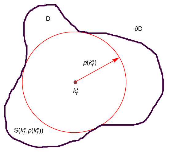
Figure 1. The largest circle $S(k^{\ast ,f},\rho \left(k^{\ast ,f}\right))$ inscribed in a region D.

Remark 5. 

Analogous to a best performance point, a least fragile point also depends on the set D chosen, and might not exist without additional conditions over D. Since $K_{a,\sigma }^0\subseteq K_{a,0}^0$ for $\sigma \le 0$, we obtain the least fragile point $k^{\ast ,f}$ for two types of sets: the global case $D\subseteq K_{a,0}^0$, and the local case $D\subseteq K_{a,\sigma }^0,\sigma <0$. In both cases, identifying this point constitutes a non-trivial analytical challenge, contrary to initial intuitive expectations. Nevertheless, the following theorem establishes a specific scenario in which the optimal point of $k^{\ast ,f}$ can be derived analytically in an exact, closed-form precision.

Proposition 5. 

Consider the quasi-polynomial (1) with $a=(0,a_1,1)$ and $a_1>0$. If $D\subset K_{a,0}^0$ is bounded by the axes τ and $k_r$, and the hyperbola $H:k_r={\displaystyle \frac{\pi a_1}{2\tau }}$, then the least fragile point is

$$k^{\ast ,f}=(\tau ,k_r)=(\rho ,\rho ),$$

(7)

where $\rho =\left(\sqrt{2}-1\right)\sqrt{\pi a_1}$ is the radius of the largest inscribed circle in D.

Proof. 

The largest circle is tangent to the boundary $\partial D$ at three points of contact. Two of them are $(\rho ,0)$ and $(0,\rho )$ which lie on the axes $\tau$ and $k_r$, respectively. The other one is $p=\left(\tau ,{\displaystyle \frac{\pi a_1}{2\tau }}\right)$ which lies on the hyperbola H. The values of $\tau$ and $\rho$ are to be determined. Since the distance from the least fragile point $(\rho ,\rho )$ to the point p is $\rho$, this number satisfies the equation

$${(\tau -\rho )}^2+{\left({\displaystyle \frac{\pi a_1}{2\tau }}-\rho \right)}^2={\rho }^2.$$

Now, since the normal line to the hyperbola H at p passes through the point $(\rho ,\rho )$, we have that

$${\displaystyle \frac{2{\tau }^2}{\pi a_1}}(\tau -\rho )+\rho ={\displaystyle \frac{\pi a_1}{2\tau }}.$$

Solving for $\tau$ and $\rho$ the foregoing equations, the result follows. □

Proposition 5 is useful and relatively simple when $\sigma =0$. However, this is not the case when $\sigma <0$, since it is necessary to perform a more extensive procedure, which has been divided according to the possible number of contact points between the circle $S(k,r)$ and the boundary $\partial D$. More details are given below.

Proposition 6. 

Suppose that the boundary $\partial D$ of the set D can be parameterized by a smooth, simple closed curve $\gamma \left(\omega \right)$ with $\omega \in I$, where I is an interval. Let $\rho \left(k\right)=min\{\parallel \gamma (\omega )-k\parallel :\omega \in I\}$ be the distance from the point k to the boundary $\partial D$, and let $J\left(k\right)=\{\omega \in I:\parallel \gamma (\omega )-k\parallel =\rho (k\left)\right\}$ be the set of all frequencies where the minimum value $\rho \left(k\right)$ is attained. Then the circle $S(k,\rho (k\left)\right)$ is tangent to the boundary $\partial D$ at each point of contact $\gamma \left(\omega \right)$ with $\omega \in J\left(k\right)$.

Proof. 

Differentiating $\parallel \gamma \left(\omega \right)-k\parallel$ with respect to $\omega$, we obtain that

$$\left[\gamma \left(\omega \right)-k\right]·{\gamma }^{\prime }\left(\omega \right)=0$$

(8)

for each frequency $\omega \in J\left(k\right)$. Thus the circle $S(k,\rho (k\left)\right)$ its tangent to the boundary at each point of contact. □

Proposition 7. 

Let γ be a smooth curve and suppose that the largest circle $S(k^{\ast ,f},\rho \left(k^{\ast ,f}\right))$ has exactly two points of contact with the boundary, say $\gamma \left({\omega }_1\right)$ and $\gamma \left({\omega }_2\right)$, where ${\omega }_1,{\omega }_2\in J\left(k^{\ast ,f}\right)$. Then the frequencies ${\omega }_1$ and ${\omega }_2$ satisfy the system of equations

$$\begin{array}{cc}\hfill \left[\gamma \left({\omega }_1\right)-\gamma \left({\omega }_2\right)\right]·{\gamma }^{\prime }\left({\omega }_1\right)& =0,\hfill \\ \hfill \left[\gamma \left({\omega }_2\right)-\gamma \left({\omega }_1\right)\right]·{\gamma }^{\prime }\left({\omega }_2\right)& =0.\hfill \end{array}$$

(9)

Proof. 

Let $\phi (k,\omega )=\parallel \gamma \left(\omega \right)-k\parallel$. We obtain Equation (9) using the fact that for this minimax problem the vector zero is in the convex hull of the set $\{\nabla \phi (k^{\ast ,f},\omega ),\omega \in J\left(k^{\ast ,f}\right)\}$, where gradient is taken with respect to the variable k. □

Equation (9) also shows that the line passing through the contact points is orthogonal to the curve at these points.

Proposition 8. 

Let γ be a smooth curve and suppose that the largest circle $S(k^{\ast ,f},\rho \left(k^{\ast ,f}\right))$ has three or more points of contact with the boundary, say $\gamma \left({\omega }_1\right),\gamma \left({\omega }_2\right)$ and $\gamma \left({\omega }_3\right)$, where ${\omega }_1,{\omega }_2,{\omega }_3\in J\left(k\right)$. Then the frequencies ${\omega }_1,{\omega }_2$ and ${\omega }_3$ satisfy the system of equations

$$\begin{array}{ccc}\hfill & & {\left\{[\gamma \left({\omega }_1\right)-\gamma \left({\omega }_2\right)]·{\gamma }^{\prime }\left({\omega }_2\right)\right\}}^2\parallel {\gamma }^{\prime }\left({\omega }_1\right){\parallel }^2-{\left\{[\gamma \left({\omega }_1\right)-\gamma \left({\omega }_2\right)]·{\gamma }^{\prime }\left({\omega }_1\right)\right\}}^2{\parallel {\gamma }^{\prime }\left({\omega }_2\right)\parallel }^2=0,\hfill \\ & & {\left\{[\gamma \left({\omega }_1\right)-\gamma \left({\omega }_3\right)]·{\gamma }^{\prime }\left({\omega }_3\right)\right\}}^2\parallel {\gamma }^{\prime }\left({\omega }_1\right){\parallel }^2-{\left\{[\gamma \left({\omega }_1\right)-\gamma \left({\omega }_3\right)]·{\gamma }^{\prime }\left({\omega }_1\right)\right\}}^2{\parallel {\gamma }^{\prime }\left({\omega }_3\right)\parallel }^2=0,\hfill \\ \hfill & & {\left\{[\gamma \left({\omega }_2\right)-\gamma \left({\omega }_3\right)]·{\gamma }^{\prime }\left({\omega }_3\right)\right\}}^2\parallel {\gamma }^{\prime }\left({\omega }_2\right){\parallel }^2-{\left\{[\gamma \left({\omega }_2\right)-\gamma \left({\omega }_3\right)]·{\gamma }^{\prime }\left({\omega }_2\right)\right\}}^2{\parallel {\gamma }^{\prime }\left({\omega }_3\right)\parallel }^2=0.\hfill \end{array}$$

(10)

Proof. 

Suppose that $\gamma :I\to {\mathbb{R}}^2$ is a simple closed curve, and let $S(k,\rho )$ be a circle with center k and radius $\rho$ inside the curve $\gamma$. Let us also assume that $S(k,\rho )$ is tangent to the curve $\gamma$ at three distinct points $\gamma \left({\omega }_1\right),\gamma \left({\omega }_2\right)$ and $\gamma \left({\omega }_3\right)$. Then using the normal vectors at these points we can write k in three different ways, leading to a system of three equations with three unknowns: ${\omega }_1,{\omega }_2$ and ${\omega }_3$. Now using the relationship between tangent and normal vectors, the system can be transformed into (10). □

The largest circle inscribed in a region D does not need to be unique, and it may have two or more points of contact with the boundary curve.

Remark 6. 

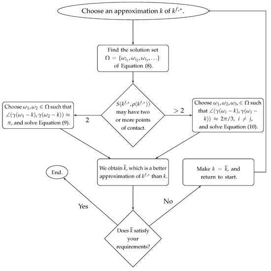
To determine $k^{\ast ,f}$ and $\rho \left(k^{\ast ,f}\right)$, follow the steps of the algorithm described below. For clarity, the algorithm is summarized in the flowchart in Figure 2.

Figure 2. Flow chart for numerical procedure.

(i) 

Choose an approximation k of $k^{\ast ,f}$, and solve Equation (8). Let $\mathrm{\Omega }=\{{\omega }_{i_1},{\omega }_{i_2},{\omega }_{i_3},\dots \}$ be the solution set. Some of these solutions may not correspond to contact points.

(ii) 

If $S(k^{\ast ,f},\rho \left(k^{\ast ,f}\right))$ has two points of contact, choose ${\omega }_1,{\omega }_2\in \mathrm{\Omega }$ in such a way that the angle between the vectors $\gamma \left({\omega }_1\right)-k$ and $\gamma \left({\omega }_2\right)-k$ is close to π radians. Then take these frequency values as an initial approximation for solving numerically system (9).

(iii) 

If $S(k^{\ast ,f},\rho \left(k^{\ast ,f}\right))$ has more than two points of contact, choose ${\omega }_1,{\omega }_2,{\omega }_3\in \mathrm{\Omega }$ in such a way that the angle among the vectors $\gamma \left({\omega }_1\right)-k,\gamma \left({\omega }_2\right)-k$ and $\gamma \left({\omega }_3\right)-k$ is close to $2\pi /3$ radians. Then take these frequency values as an initial approximation for solving numerically system (10).

(iv) 

Repeat steps (i)–(iii) until satisfied.

Systems (8)–(10) may be solved numerically by using Newton’s method.

6. Greatest Robustness Point

In this section, we obtain the gains for the most robust controller.

The parameters of the system can be treated in a similar way to the control gains. For a fixed $k\in K$, the curve

$${\mathrm{\Gamma }}_k=\{a\in A:q(a,k,s)=0\mathrm{for}\mathrm{some}s=i\omega \}$$

splits A into subregions where the quasi-polynomial (1) has a constant number of roots with positive real part. That is

$$A=A_k^0\cup A_k^1\cup A_k^2\cup \cdots ,$$

where

$$\begin{array}{cc}\hfill A_k^m=\{& a\in A:q(a,k,s)\mathrm{has}\mathrm{exactly}m\mathrm{roots}\mathrm{with}\mathrm{positive}\mathrm{real}\mathrm{part}\}.\hfill \end{array}$$

Now, the set $A_k^0$ is the robustness region of the quasi-polynomial (1), and we have that ${\mathrm{\Gamma }}_k=\partial A_k^0$.

Definition 5. 

For a fixed $k\in K$, let E be a subset of $A_k^0$ such that $\partial E\subset {\mathrm{\Gamma }}_k$. A point of greatest robustness of a systems is a set of parameters $a^{\ast ,r}\in E$ with the largest distance to the boundary $\partial E$. This point satisfies

$$\rho \left(a^{\ast ,r}\right)=sup\{\rho \left(a\right):a\in E\},$$

where $\rho \left(a\right)=inf\{\parallel l-a\parallel :l\in \partial E\}$ is the distance from the point a to the boundary $\partial E$.

Next, we obtain the curves ${\mathrm{\Gamma }}_k$ to delimit the stability region $A_k^0$ of quasi-polynomial (1).

Proposition 9. 

Consider the quasi-polynomial (1), and suppose that $k=(\tau ,k_r)$ is fixed. The parametric equations of the curve ${\mathrm{\Gamma }}_k$ which bounds the robustness region $A_k^0$ are the following.

(i) 

If $\omega =0$, we obtain the vertical line $a_0=-a_2{k}_r$.

(ii) 

If $\omega \ne 0$, then $a_0=-a_2{k}_{r}cos\left(\tau \omega \right)$ and $a_1={\displaystyle \frac{a_2{k}_r}{\omega }}sin\left(\tau \omega \right)$.

Proof. 

Line (i) is obtained by evaluating (1) at $s=0$, and solving for $a_0$. While the parametric equations (ii) are obtained by evaluating (1) at $s=i\omega$, and solving for $a_0$ and $a_1$. □

The following result provides an approach for the computation of $a^{\ast ,r}$.

Proposition 10. 

Consider the quasi-polynomial (1), and suppose that $k=(\tau ,k_r)$ is fixed. If $a_0=0$ and $a_2$ is given, then the robustness interval is

$$a_1\in \left({\underline{a}}_1,+\infty \right)\subset A_k^0,$$

(11)

where ${\underline{a}}_1={\displaystyle \frac{2\tau a_2{k}_r}{\pi }}sin\left({\displaystyle \frac{\pi }{2}}\right)$. Furthermore, choosing a compact set $E=\left[{\underline{a}}_1,{\overline{a}}_1\right]$, where ${\overline{a}}_1$ is proposed by the user, we have that

$$a^{\ast ,r}=a_1^{\ast ,r}={\displaystyle \frac{{\overline{a}}_1+{\underline{a}}_1}{2}}.$$

(12)

Proof. 

This result is obtained using (ii) of Proposition 9 and substituting $\tau \omega ={\displaystyle \frac{\pi }{2}}$. □

From the previous result, we can observe that the robustness depends on the controller gains, thus the gains can be used to maximize the robustness of the system. Furthermore, it is easy to infer the following.

Remark 7. 

If $r:=a_1^{-1}$ and $a_1$ satisfies (11), then

$$\begin{array}{c}\hfill r\in \left(0,{\underline{a}}_1^{-1}\right),\mathrm{and}{r}^{\ast ,r}:={\left(a_1^{\ast ,r}\right)}^{-1}={\displaystyle \frac{a_1^{-1}}{2}}.\end{array}$$

(13)

Since the greatest robustness point $a^{\ast ,r}$ shares the same properties as a least fragile point, we can apply Propositions 6–8 to obtain these points in the corresponding regions $A_k^0$.

7. Relationship Among Performance, Fragility and Robustness

Previous sections have presented theoretical results for determining the performance, fragility, and robustness properties of systems characterized by the quasi-polynomial (1). As noted in the problem statement, it is essential to establish conditions under which system stability is maintained in the presence of both independent parameter variations and gain perturbations. However, a comprehensive analysis also requires simultaneous examination of stability regions as functions of both parameters and gains, enabling the determination of performance and stability invariance in the system response. The following results address these objectives.

To determine a stability region in $\tau k_r{a}_1$-space for quasi-polynomial (1) we apply the following result.

Lemma 2 

([37]). The roots of $z=c{\mathrm{e}}^z$ all lie to the right of $Re\left(z\right)=\lambda$ if and only if $\lambda <1$ and $\lambda {\mathrm{e}}^{-\lambda }<c<{\mathrm{e}}^{-\lambda }\sqrt{{\lambda }^2+{\nu }^2}$, where ν is the unique root of $\nu cot\nu =\lambda$ in the interval $(0,\pi )$.

For $\nu \in \left(0,{\displaystyle \frac{\pi }{2}}\right)$, we define the functions $c_1\left(\nu \right)=\lambda {\mathrm{e}}^{-\lambda }$ and $c_2\left(\nu \right)={\mathrm{e}}^{-\lambda }\sqrt{{\lambda }^2+{\nu }^2}$, where $\lambda =\nu cot\nu$. The graphs of these functions are shown in Figure 3.

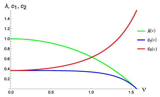
Figure 3. Functions $c_1,c_2$ and $\lambda$.

Proposition 11. 

Let $\nu \in \left(0,{\displaystyle \frac{\pi }{2}}\right)$ be fixed, and consider the quasi-polynomial (1), with $a=(0,a_1,1)$ and $a_1\ne 0$. If the positive quantities $\tau ,k_r$ and $a_1$ satisfy the inequality

$$c_1\left(\nu \right)<{\displaystyle \frac{\tau k_r}{a_1}}<c_2\left(\nu \right),$$

(14)

then the quasi-polynomial (1) is stable.

Proof. 

If $a_0=0$ and $a_2=1$, the quasi-polynomial (1) becomes

$$q(a,k,s)=a_{1}s+k_r{\mathrm{e}}^{-\tau s}.$$

(15)

Making the change of variable $z=-\tau s$, $\tau >0$, and applying Lemma 2, we obtain that all the roots of quasi-polynomial (15) lie to the left of $\mathrm{Re}\left(s\right)=-{\displaystyle \frac{\lambda }{\tau }}$ if and only if the inequality

$$\lambda {\mathrm{e}}^{-\lambda }<{\displaystyle \frac{\tau k_r}{a_1}}<{\mathrm{e}}^{-\lambda }\sqrt{{\lambda }^2+{\nu }^2}.$$

(16)

holds. Now using the definitions of functions $c_1$ and $c_2$ in (16) we obtain (14). □

For $a=(0,a_1,1)$ and $\lambda \in (0,1)$, denote by $R\left(\nu \right)$ the corresponding region in $\tau k_r{a}_1$-space defined by inequality (14).

Proposition 12. 

If $a=(0,a_1,1)$, and $\lambda \in (0,1)$, then

$$inf\{\alpha (a,k):(a_1,k_r,\tau )\in R\left(\nu \right)\}=-\infty ,$$

(17)

where

$$\alpha (a,k)=sup\left\{\mathrm{Re}\right(s):q(a,k,s)=0\}.$$

Proof. 

We have that

$$\alpha (a,k)\le -{\displaystyle \frac{\lambda }{\tau }}\mathrm{for} \mathrm{all}(a_1,k_r,\tau )\in R\left(\nu \right),$$

(18)

and we need to verify the inequality

$$c_1\left(\nu \right)<{\mathrm{e}}^{-1}<c_2\left(\nu \right)for\nu \in \left(0,{\displaystyle \frac{\pi }{2}}\right).$$

(19)

Since $\lambda$ and $\nu$ are interchangeable variables, (19) is quivalent to say that

$$\phi \left(\lambda \right)=\lambda -{\mathrm{e}}^{\lambda -1}<0for\lambda \in (0,1)$$

(20)

and

$$\psi \left(\nu \right)=\nu csc\nu -{\mathrm{e}}^{\nu cot\nu -1}<0for\nu \in \left(0,{\displaystyle \frac{\pi }{2}}\right).$$

(21)

Using calculus, inequalities (20) and (21) are readily stated. Thus the unbounded region $R\left(\nu \right)$ contains the surface ${\displaystyle \frac{\tau k_r}{a_1}}={\mathrm{e}}^{-1}$, and there is not a finite value for the spectral abscissa of the quasi-polynomial $q(a,k,s)$ in this region. □

8. Implementation of the Theoretical Results

Next, without loss of generality, we implement the theoretical results presented above on an experimental platform consisting of an omnidirectional mobile robot.

8.1. Description of the Experimental Platform

The OMR is built using three 12[V] POLOLU 37D gearmotors, with a gear ratio 1:70 and encoder with a resolution of 64 counts per revolution, and wheels with radius $r=0.03$ [m], see Figure 4. An STM32F4 Discovery (^© STMmicroelectronics, Geneva, Switzerland) board is used as a data acquisition card and the communication between the computer and the robot is realized in real-time using the public and available Waijung 1 (STM32 target 2018 for ^©Matlab, Natick, MA, USA) library via Bluetooth using an ESP32 microcontroller ^© Espressif Systems, Shanghai, China. The setup runs inside an indoor environment with a set of 10 infrared ^© Vicon Motion Systems Ltd., Oxford, UK cameras with precision of $0.5$ [mm] which measure the position and orientation of each robot in an area of $5\times 4$ [m] with a sample time of $0.005$ [s]. The robot has several reflective markers with different patterns, in order to be detected by the TRACKER 3.0 software,^© Vicon Motion Systems Ltd, Oxford, UK.

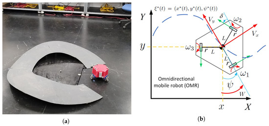
Figure 4. OMR experimental platform. (a) OMR with disturbance (ramp). (b) Notation in the considered OMR.

To corroborate the theoretical results, we determine performance, fragility and robustness of the OMR for a trajectory tracking task in the $xy$-plane, using the experimental platform described below. Here the kinematic model (22) is considered. For tuning the delayed-action controller (25), a quasi-polynomial of the form (1), where $a=(0,a_1,1)$ with $a_1=r^{-1}=33.333$, is used.

The control objective is a trajectory tracking task of the OMR position in the $xy$-plane. The reference signal is a circle of radius 0.5 [m], which will be denoted by Ref.

To illustrate the effectiveness of tracking in the presence of external disturbances, a ramp is utilized to change the surface of the path traveled, see Figure 4a. While to quantify the efficiency in the tracking task, the mean square error (MSE) index is obtained.

8.2. Kinematic Model of the OMR

An OMR is a mobile vehicle with mecanum or omnidirectional wheels that allow it to move in any direction instantly and increase the maneuverability of the robot. The system has three independent control inputs, which can be decoupled to control its three degrees of freedom fully $\left[xy\psi \right]$. This feature is not present in other mobile robots, such as differential or Ackerman steering robots, which have only two control inputs involving non-holonomic constraints [38].

A kinematic model of the OMR, schematized in Figure 4b, is of the form

$$\underset{\dot{\xi }}{\underbrace{\left[\begin{array}{c}\dot{x}\\ \dot{y}\\ \dot{\psi }\end{array}\right]}}=\underset{R\left(\psi \right)}{\underbrace{\left[\begin{array}{ccc}cos\left(\psi \right)& -sin\left(\psi \right)& 0\\ sin\left(\psi \right)& cos\left(\psi \right)& 0\\ 0& 0& 1\end{array}\right]}}\underset{U}{\underbrace{\left[\begin{array}{c}{V}_x\\ V_y\\ W\end{array}\right]}},$$

(22)

where $(x,y)\in {\mathbb{R}}^2$ represents the robot position in the plane, $\psi \in \mathbb{R}$ is the robot orientation angle, and $V_x,V_y,W\in \mathbb{R}$ are the longitudinal, lateral, and angular velocities, respectively. The term R$\left(\psi \right)$ represents the non-singular rotation matrix around the Z axis and U is the control input vector.

In order to implement a controller, the following transformation of robot velocities U to velocities of OMR wheels $\mathrm{\Omega }$ is required

$$\underset{\mathrm{\Omega }}{\underbrace{\left[\begin{array}{c}{\omega }_1\left(t\right)\\ {\omega }_2\left(t\right)\\ {\omega }_3\left(t\right)\end{array}\right]}}={\displaystyle \frac{1}{r}}\underset{R\left(\delta \right)}{\underbrace{\left[\begin{array}{ccc}-sin\left(\delta \right)& cos\left(\delta \right)& L\\ -sin\left(\delta \right)& -cos\left(\delta \right)& L\\ 1& 0& L\end{array}\right]}}\underset{U}{\underbrace{\left[\begin{array}{c}{V}_x\\ V_y\\ W\end{array}\right]}},$$

(23)

where L is the distance from any wheel to the center of mass of the robot, r is the radius of the wheel and $\delta ={\displaystyle \frac{\pi }{6}}$, see Figure 4b. Thus, solving (23) for U and substituting into (22), we have

$$\dot{\xi }=rR\left(\psi \right)R{\left(\delta \right)}^{-1}\mathrm{\Omega }.$$

(24)

Now, we propose the following novel nonlinear controller with delayed-action, which will be called delayed nonlinear controller (D-NLC):

$$\mathrm{\Omega }=R\left(\delta \right)R{\left(\psi \right)}^{-1}\left[{\displaystyle \frac{1}{r}}{\dot{\xi }}^{\ast }-K_r{e}_{\xi }(t-\tau )\right],$$

(25)

where $\tau \in {\mathbb{R}}^{+}$ is the time-delay, $K_r=k_r{I}_3$, with $k_r\in \mathbb{R}$ and $I_3\in {\mathbb{R}}^{3\times 3}$ is the identity matrix, and $e_{\xi }\left(t\right)=\xi \left(t\right)-{\xi }^{\ast }\left(t\right)\in {\mathbb{R}}^3$, whith ${\xi }^{\ast }\left(t\right)$ is the desired vector of position and orientation of the robot. From (25) and (24), the close-loop error dynamic is

$$\dot{e_{\xi }}\left(t\right)=-r{K}_r{e}_{\xi }(t-\tau ).$$

(26)

Defining $a_1=1/r$, the characteristic equation of this dynamics is

$$\begin{array}{cc}\hfill Q(a,k,s)& =\sum _{j=0}^3{p}_j\left(s\right){\mathrm{e}}^{-{\tau }_{j}s}=0.\hfill \end{array}$$

(27)

Here, $p_0\left(s\right)=a_1^3{s}^3$, $p_1\left(s\right)=3a_1^2{k}_r{s}^2$, $p_2\left(s\right)=3a_1{k}_r^{2}s$, $p_3\left(s\right)=k_r^3$, ${\tau }_0=0$, ${\tau }_1=\tau$, ${\tau }_2=2\tau$, and ${\tau }_3=3\tau$. Note that (27) is a quasi-polynomial of degree 9 with commensurable delays, see [39]. However, (27) can be written as the product of three quasi-polynomials of degree 2 of the form

$$q(a,k,s)=a_{1}s+k_r{\mathrm{e}}^{-\tau s}.$$

(28)

Namely,

$$Q(a,k,s)={\left[q(a,k,s)\right]}^3.$$

Thus, thanks to the OMR modeling structure suggested in (22) and (23), the novel delayed nonlinear controller proposed in (25) and some simple but strategic algebraic manipulations, we can now streamline/guarantee OMR trajectory tracking in the event of variations in controller gains and vehicle parameters using the results given in the previous sections on the quasi-polynomial (28). This framework will serve to validate the efficacy and relevance of our proposed control strategy.

8.3. General Scheme to Obtain Performance, Fragility and Robustness of the OMR

In this section the theoretical results are applied to obtain best performance, least fragile and greatest robustness points for the OMR. The steps are as follow.

For steps S1 to S4, fix $a=(0,33.333,1)$, and for steps S5–S6, fix $k=(0.0625,196.20)$.

S1.

Use Proposition 1 to determine the $\sigma$-stability regions $K_{a,\sigma }^0$, $\sigma \le 0$. For $n=0$, Figure 5 shows the stability region $K_{a,0}^0$ ($--$) obtained by using (i)–(iii) of Proposition 1, and the $\sigma$-stability regions $K_{a,\sigma }^0$ (—) and (—), with $\sigma =-1,-6,-13,-15,-16,-18$, obtained by using (iv)-(v) of Proposition 1. Figure 5 also shows the singular points obtained by (5) for several values of $\sigma$, see Remark 4.

S2.

Choose a compact set $D\subseteq K_{a,\sigma }^0$ for some $\sigma <0$ or $\sigma =0$.

(a)

If $\sigma =0$, pick a compact set $D\subset K_{a,0}^0$ bounded by a vertical line $\tau =t$, and a horizontal line $k_r=\kappa$ as indicated in Figure 6a.

(b)

If $\sigma <0$, pick a compact set $D\subset K_{a,\sigma }^0$ delimited by the $\sigma$-stability region $K_{a,\sigma }^0$ and a horizontal line $k_r=\kappa$ as indicated in Figure 6b.

S3.

Obtaining the best performance point $k^{\ast ,p}$ of a set $D\subset K_{a,\sigma }^0$, $\sigma \le 0$. Usually, this point is obtained geometrically, but it can be obtained analytically using Formulas (5) and (6) or Proposition 4. Some points $k^{\ast ,p}$ are given in Table 1 for some values of $\sigma <0$.

S4.

The least fragile point $k^{\ast ,f}$ of a set $D\subset K_{a,\sigma }^0$, $\sigma \le 0$, can be obtained by using the algorithm described in Remark 6. Without loss of generality, we illustrate this algorithm for two values of $\sigma$.

(a)

For $\sigma =0$, Figure 7a shows the set D bounded by the straight lines $\tau =0$, $k_r=0$, and the hyperbola (iii), which is inside the stability region $K_{a,0}^0$. Here, the least fragile point is $k^{\ast ,f}=(4.23874,4.23874)$ and $\rho =4.23874$.

(b)

For $\sigma =-6$, Figure 7b shows the set D bounded by the axis $k_r$, and the curves (iii) and (iv), which is inside the $\sigma$-stability region $K_{a,\sigma }^0$. Here, the least fragile point is $k^{\ast ,f}=(0.0527804,199.998)$ and $\rho =0.0527804$.

S5.

Use Proposition 9 to determine the robustness region $A_k^0$. For illustrative purposes and without loss of generality, Figure 8 shows a representative robustness region of quasi-polynomial (1) when $a_2=1$.

S6.

Obtaining the greatest robustness point $a^{\ast ,r}$ of the chosen set $E\subset A_k^0$, using (12) from Proposition 10 or (13) from Remark 7.

S7.

Finally, Figure 9 shows the finite portion of the stability region $R\left(1.34\right)$ in $\tau k_r{a}_1$-space, which is inside the box $B=\{0\le \tau \le 0.1,160\le k_r\le 222,1.8\le a_1\le 34\}$. See Proposition 11.

Figure 5. $\sigma$-stability regions for quasi-polynomial (1).

Figure 6. Choosing a compact set D. (a) Compact set $D\subset K_{a,0}^0$. (b) Compact set $D\subset K_{a,\sigma }^0$, $\sigma =-6$.

Figure 7. Finding the least fragile point. (a) The least fragile point of region D. (b) The least fragile point $k^{\ast ,f}\in D$ for $\sigma =-6$.

Figure 8. Robustness region of the quasi-polynomial (1) in plane $a_0$–$a_1$ with $a_2$ fixed.

Figure 9. The finite portion $R\left(1.34\right)\cap B$ of the stability region $R\left(1.34\right)$ in $\tau k_r{a}_1$-space. (a) Vertex $V=(0.1,160,15.9255)$ in blue, and sphere with center $k_{3D}^{\ast }=(0.075,191,28)$ and radius $\rho =0.025$ in red. (b) Zoom in of the red sphere in (a).

8.4. Validation and Implementation of Results

This section presents experimental validation of the theoretical framework developed in previous sections, implemented on the OMR platform.

8.4.1. Experimental Tests of OMR Performance

The best performance points $k^{\ast ,p}$ of the OMR are obtained using (5), as described in step S3 from Section 8.3. Table 1 shows the controller gains $k^{\ast ,p}=(\tau ,k_r)$ for a given $\sigma <0$.

Figure 10a shows the performance of the OMR without a disturbance (ramp) in a tracking task, Ref ($--$), using three points $k^{\ast ,p}$ from Table 1 to tune the delayed-action of the controller (25). Figure 10b shows the performance of the OMR using the same points as in Figure 10a, but with a disturbance (ramp). In addition, Table 1 shows the mean square error (MSE) between the desired position (Ref) and the OMR response. Some videos on the performance of the OMR, when $k=(0.055,220.72)$, can be found at the following links: https://drive.google.com/file/d/14C6eixNj5i5PK3lx7KYzKSEyu4rZoLgz/view?usp=sharing (accessed on 20 August 2025), with platform and https://drive.google.com/file/d/1ak1oBaItJgwGHSGs8Hq1kOPKKQ03zXTg/view?usp=sharing (accessed on 20 August 2025), without platform.

Table 1. The best performance points $k^{\ast ,p}$ for a $\sigma$-stability region and MSE between OMR and Ref, with $a=(0,33.333,1)$ fixed.

$\mathit{\sigma }$ Given	${\mathit{k}}^{\ast ,\mathit{p}}=(\mathit{\tau },{\mathit{k}}_{\mathit{r}})$	MSE of Figure 10a,	MSE of Figure 10b,
	Obtained	w/o Ramp, [m]	w Ramp, [m]
$-13$	$(0.0769,159.41)$	$0.0043$	$0.0054$
$-16$	$(0.0625,196.20)$	$0.0026$	$0.0037$
$-18$	$(0.0555,220.72)$	$0.0028$	$0.0043$

Table 1. The best performance points $k^{\ast ,p}$ for a $\sigma$-stability region and MSE between OMR and Ref, with $a=(0,33.333,1)$ fixed.

$\mathit{\sigma }$ Given	${\mathit{k}}^{\ast ,\mathit{p}}=(\mathit{\tau },{\mathit{k}}_{\mathit{r}})$	MSE of Figure 10a,	MSE of Figure 10b,
	Obtained	w/o Ramp, [m]	w Ramp, [m]
$-13$	$(0.0769,159.41)$	$0.0043$	$0.0054$
$-16$	$(0.0625,196.20)$	$0.0026$	$0.0037$
$-18$	$(0.0555,220.72)$	$0.0028$	$0.0043$

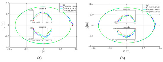
Figure 10. OMR position performance in the $xy$-plane. (a) Without disturbance/ramp. (b) With disturbances/ramp.

8.4.2. Experimental Tests of OMR Fragility

Figure 11 shows the position of the OMR, without ramp, using the least fragile points $k^{\ast ,f}=(\tau ,k_r)$ from Table 2 to tune the delayed-action of the controller (25), as described in step S4 from Section 8.3. For $\sigma =0$, $k^{\ast ,f}$ is obtained by applying Proposition 5, while for $\sigma =-0.27,-0.48$ and $\sigma =-6$, the (local) least fragile points of the closed $\sigma$-stability regions are obtained by applying the numerical procedure mentioned in Remark 6, see Figure 7b.

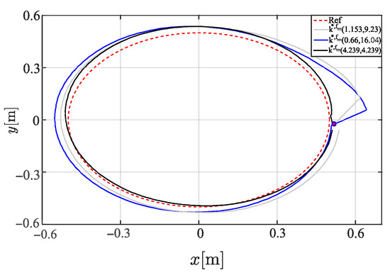
Figure 11. OMR position fragility in the $xy$-plane using the parameters given in Table 2.

Table 2. The least fragile points for a $\sigma$-stability region and MSE between OMR and Ref, with $a=(0,33.333,1)$ fixed.

$\mathit{\sigma }$ Given	${\mathit{k}}^{\ast ,\mathit{f}}=(\mathit{\tau },{\mathit{k}}_{\mathit{r}})$	MSE of Figure 11,
	Obtained	w/o Ramp, [m]
0	$(4.2387,4.2387)$	$0.0221$
$-0.27$	$(1.1527,9.2304)$	$0.0496$
$-0.48$	$(0.6585,16.0426)$	$0.0532$

As expected, poor performance is observed, since the exponential decay rate $\sigma$ is close to zero. However, due to the proposed analysis, a less fragility to variations in the gains of the delayed-action of the controller (25) is guaranteed. Table 2 shows that the closer $\sigma$ to zero the less fragile the controller. Also shows the MSE obtained between the OMR response and the desired position Ref.

8.4.3. Experimental Tests of OMR Robustness

Next, we get the greatest robustness point using the step S6 from Section 8.3. Figure 12a depicts a robustness test of the OMR platform in closed-loop with the controller (25), when there are parametric variations. This figure shows the OMR position on $xy$-plane when $k^{\ast ,p}=(0.0769,159.41)$, and $r=a_1^{-1}\in \{0.03,0.05,0.08\}$ [m] is varied. While, Figure 12b depicts the robustness when $k^{\ast ,p}=(0.0555,220.72)$, and $r=a_1^{-1}\in \{0.03,0.05,0.08\}$ [m] is varied. Both without disturbance (ramp). Table 3 presents the MSE between the desired position (Ref) and the OMR response, due to the variation of the parameter $a_1$.

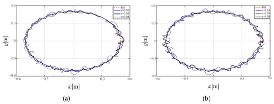
Figure 12. OMR robustness. (a) $k^{\ast ,p}=(0.0769,159.41)$ and varying $r=a_1^{-1}=0.03,0.05,0.08$. (b) $k^{\ast ,p}=(0.0555,220.7)$ and varying $r=a_1^{-1}=0.03,0.05$, $0.08$.

Table 3. The greatest robustness point and MSE between OMR and Ref, with $k=(\tau ,k_r)$ fixed.

$\mathit{k}=(\mathit{\tau },{\mathit{k}}_{\mathit{r}})$	Robustness	Greatest Robustness	MSE	MSE	MSE
Given	Interval	Point	$\mathit{r}=\mathbf{0.03}$	$\mathit{r}=\mathbf{0.05}$	$\mathit{r}=\mathbf{0.08}$
$(0.0769,159.41)$	$r\in (0,0.128138)$ [m]	$r^{\ast ,r}=0.064069$ [m]	$0.0043$	$0.0131$	$0.0231$
$(0.0555,220.72)$	$r\in (0,0.128228)$ [m]	$r^{\ast ,r}=0.064114$ [m]	$0.0028$	$0.018$	$0.025$

8.4.4. Experimental Tests of OMR in $\tau k_r{a}_1$-Space

Figure 9 depicts a portion of the robust stability region $R\left(1.34\right)$ in $\tau k_r{a}_1$-space, as described in step S7 from Section 8.3. To corroborate the veracity of this region, Figure 13 shows the OMR position using an approximation of the non-fragile point $k_{3D}^{\ast }=(0.075,191,28)$ of $R\left(1.34\right)$ (with radius $\rho =0.025$), Figure 14a using the vertex point $V=(0.1,160,15.9255)$, and Figure 14b the point $W=(0.5,191,10)$ outside of the region $R\left(1.34\right)$.

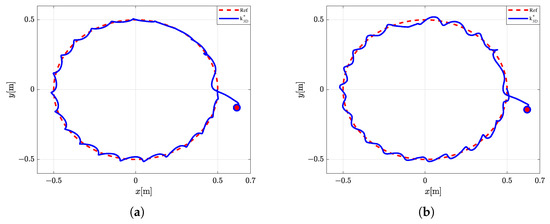
Figure 13. OMR position using the point $k_{3D}^{\ast }=(0.075,191,28)$ of the region $R\left(1.34\right)$ given in Figure 9b. (a) Without disturbance/ramp. (b) With disturbances/ramp.

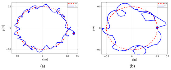
Figure 14. OMR position using the points V and W of the region $R\left(1.34\right)$ given in Figure 9a, without disturbances/ramp. (a) $V=(0.1,160,15.9255)$. (b) $W=(0.5,191,10)$.

8.5. Comparison: D-NLC vs. P-NLC

As extensively discussed in previous sections, incorporating time-delay elements in controllers can enhance system response performance and attenuate control signal noise. To validate these advantages, we propose a natural and fair performance comparison between our proposed controller (25) and controllers of the form:

$$\begin{array}{c}\hfill \mathrm{\Omega }:={\mathrm{\Omega }}_i=R\left(\delta \right)R{\left(\psi \right)}^{-1}\left[{\displaystyle \frac{1}{r}}{\dot{\xi }}^{\ast }-u_i\left(t\right)\right],i=1,2,3;\end{array}$$

(29)

where $u_1\left(t\right)=K_d{\dot{e}}_{\xi }$, $u_2\left(t\right)=K_i{\int }_0^{\infty }{e}_{\xi }\left(\varsigma \right)d\varsigma$ and $u_3\left(t\right)=K_p{e}_{\xi }$ are classical controllers. Here, $K_d=k_d{I}_3$, $K_i=k_i{I}_3$, and $K_p=k_p{I}_3$, with $k_d,k_i,k_p\in \mathbb{R}$.

Remark 8. 

Note that the nonlinear controller (29), with a derivative-action $u_1\left(t\right)=K_d{\dot{e}}_{\xi }$, or with an integral-action $u_2\left(t\right)=K_i{\int }_0^{\infty }{e}_{\xi }\left(\varsigma \right)d\varsigma$ are not suitable for ensuring the tracking of trajectories of the system (24).

Because of this, we use the nonlinear controller (29) with a proportional action $u_3\left(t\right)=K_p{e}_{\xi }$, which we call proportional nonlinear controller (P-NLC). It seems to be the only option to make the corresponding comparison. Thus, note that the closed-loop systems (24) with P-NLC is of the form

$$\begin{array}{c}\hfill a_1{\dot{e}}_{\xi }\left(t\right)=-K_p{e}_{\xi }\left(t\right),\end{array}$$

whose characteristic equation is

$$\begin{array}{cc}\hfill Q_p(a,k,s)& ={\left[p(a,k,s)\right]}^3=0.\hfill \end{array}$$

where

$$p(a,k,s)=a_{1}s+k_p.$$

(30)

To ensure an equitable comparison, the gain $k_p$ of the proportional-action is tuned to match the performance level $\sigma$ achieved by the proposed delayed-action, i.e., the dominant roots of (28) and (30) are placed on the vertical line $\mathrm{Re}\left(s\right)=\sigma <0$. Thus

$$k_p=-a_1·\sigma .$$

(31)

Figure 15 shows the OMR position using the D-NLC and P-NLC controllers, both controllers tuned to obtain a performance of $\sigma =-13$ in the closed-loop system response. Here, $k^{\ast ,p}=(0.0769,159.41)$ is taken from Table 1 and $k_p=433.3$ is obtained from (31). A similar behavior in the performance of the OMS is observed when we tune the controlled for $\sigma =-16$ and $\sigma =-18$, respectively.

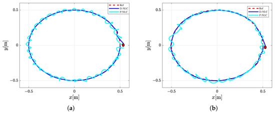
Figure 15. Comparison when $\sigma =-13$: $k^{\ast ,p}=(0.0769,159.41)$ and $k_p=433.3$. (a) Without disturbance/ramp. (b) With disturbances/ramp.

Remark 9. 

Comparisons of robustness and fragility properties are beyond the scope of this work, since these two properties will not be determined here for controllers of the form (29). However we have highlighted this as a key area for future investigation.

9. Conclusions

This manuscript presents an exhaustive analysis to jointly determine performance, fragility and robustness on a class of quasi-polynomial of degree 2. Derived from this analysis, necessary and sufficient conditions are given to obtain the controller gains that provide best performance $k^{\ast ,p}\in K$ and least fragility $k^{\ast ,f}\in K$, as well as the most robust parametric point $a^{\ast ,r}\in A$. Furthermore, as an interconnection between the properties of performance, fragility and robustness, we propose necessary and sufficient conditions to determine the invariance capacity in stabilizing the closed-loop system response in the $\tau k_r{a}_1$-space. The proposed theoretical results are satisfactorily validated by experimental tests on an OMR in trajectory tracking tasks using an advanced optical motion capture system (^©Vicon Motion Systems Ltd, Oxford, UK). Furthermore, the experimental implementations and comparative analysis presented in this contribution demonstrate that our approach provides both a more efficient tuning alternative for delayed controllers and a promising alternative for robotic system control applications.

References

- Bhattacharyya, S.P.; Keel, L.H. Robust control: The parametric approach. In Advances in Control Education 1994; Prentice-Hall Information and System Sciences Series; Prentice Hall PTR: London, UK, 1995; pp. 49–52. [Google Scholar]
- Alfaro, V.M. PID controllers’ fragility. ISA Trans. 2007, 46, 555–559. [Google Scholar] [CrossRef]
- Zouaoui, S.; Mohamed, E.; Kouider, B. Easy tracking of UAV using PID controller. Period. Polytech. Transp. Eng. 2019, 47, 171–177. [Google Scholar] [CrossRef]
- Abdallah, C.; Dorato, P.; Benites-Read, J.; Byrne, R. Delayed positive feedback can stabilize oscillatory systems. In Proceedings of the American Control Conference, San Francisco, CA, USA, 2–4 June 1993; IEEE: Piscataway, NJ, USA, 1993; pp. 3106–3107. [Google Scholar]
- Bleich, M.E.; Socolar, J.E. Stability of periodic orbits controlled by time-delay feedback. Phys. Lett. A 1996, 210, 87–94. [Google Scholar] [CrossRef]
- Haddad, W.M.; Kapila, V.; Abdallah, C.T. Stabilization of linear and nonlinear systems with time delay. In Stability and Control of Time-Delay Systems; Springer: Berlin/Heidelberg, Germany, 1998; pp. 205–217. [Google Scholar]
- Niculescu, S.I.; Abdallah, C.T. Delay effects on static output feedback stabilization. In Proceedings of the 39th IEEE Conference on Decision and Control (Cat. No. 00CH37187), Sydney, NSW, Australia, 12–15 December 2000; IEEE: Piscataway, NJ, USA, 2000; Volume 3, pp. 2811–2816. [Google Scholar]
- Ulsoy, A.G. Time-delayed control of SISO systems for improved stability margins. J. Dyn. Syst. Meas. Control 2015, 137, 041014. [Google Scholar] [CrossRef]
- Suh, I.; Bien, Z. Proportional minus delay controller. IEEE Trans. Autom. Control 1979, 24, 370–372. [Google Scholar] [CrossRef]
- Suh, H.; Bien, Z. Use of time-delay actions in the controller design. IEEE Trans. Autom. Control 1980, 25, 600–603. [Google Scholar] [CrossRef]
- Mondie, S.; Villafuerte, R.; Garrido, R. Tuning and noise attenuation of a second order system using Proportional Retarded control. IFAC Proc. Vol. 2011, 44, 10337–10342. [Google Scholar] [CrossRef]
- Niculescu, S.I.; Gu, K.; Abdallah, C.T. Some remarks on the delay stabilizing effect in SISO systems. In Proceedings of the American Control Conference, Denver, CO, USA, 4–6 June 2003; IEEE: Piscataway, NJ, USA, 2003; Volume 3, pp. 2670–2675. [Google Scholar]
- Özbek, N.S.; Eker, İ. Investigation of time-delayed controller design strategies for an electromechanical system. In Proceedings of the 2017 4th International Conference on Electrical and Electronic Engineering (ICEEE), Ankara, Turkey, 8–10 April 2017; IEEE: Piscataway, NJ, USA, 2017; pp. 181–186. [Google Scholar]
- Villafuerte, R.; Mondié, S.; Vazquez, C.; Collado, J. Proportional retarded control of a second order system. In Proceedings of the 2009 6th International Conference on Electrical Engineering, Computing Science and Automatic Control (CCE), Toluca, Mexico, 10–13 January 2009; IEEE: Piscataway, NJ, USA, 2009; pp. 1–6. [Google Scholar]
- Ramírez, A.; Mondié, S.; Garrido, R.; Sipahi, R. Design of proportional-integral-retarded (PIR) controllers for second-order LTI systems. IEEE Trans. Autom. Control 2016, 61, 1688–1693. [Google Scholar] [CrossRef]
- Boussaada, I.; Unal, H.U.; Niculescu, S.I. Multiplicity and stable varieties of time-delay systems: A missing link. In Proceedings of the 22nd International Symposium on Mathematical Theory of Networks and Systems (MTNS), Minneapolis, MN, USA, 12–15 July 2016; pp. 1–6. [Google Scholar]
- Oaxaca-Adams, G.; Villafuerte-Segura, R. On controllers performance for a class of time-delay systems: Maximum decay rate. Automatica 2023, 147, 110669. [Google Scholar] [CrossRef]
- Ma, D.; Boussaada, I.; Chen, J.; Bonnet, C.; Niculescu, S.I.; Chen, J. PID control design for first-order delay systems via MID pole placement: Performance vs. robustness. Automatica 2022, 137, 110102. [Google Scholar] [CrossRef]
- Michiels, W.; Niculescu, S.I.; Boussaada, I.; Mazanti, G. On the relations between stability optimization of linear time-delay systems and multiple rightmost characteristic roots. Math. Control. Signals, Syst. 2025, 37, 143–166. [Google Scholar] [CrossRef]
- Torres-García, D.; Méndez-Barrios, C.F.; Niculescu, S.I. Stabilization of second-order non-minimum phase system with delay via PI controllers. Spectral abscissa optimization. IEEE Access 2024, 12, 170851–170867. [Google Scholar] [CrossRef]
- Silva, G.J.; Datta, A.; Bhattacharyya, S. PID tuning revisited: Guaranteed stability and non-fragility. In Proceedings of the 2002 American Control Conference (IEEE Cat. No. CH37301), Anchorage, AK, USA, 8–10 May 2002; IEEE: Piscataway, NJ, USA, 2002; Volume 6, pp. 5000–5006. [Google Scholar]
- Melchor-Aguilar, D.; Niculescu, S.I. Computing non-fragile PI controllers for delay models of TCP/AQM networks. Int. J. Control 2009, 82, 2249–2259. [Google Scholar] [CrossRef]
- Morărescu, I.C.; Méndez-Barrios, C.F.; Niculescu, S.I.; Gu, K. Stability crossing boundaries and fragility characterization of PID controllers for SISO systems with I/O delays. In Proceedings of the 2011 American Control Conference, San Francisco, CA, USA, 29 June–1 July 2011; IEEE: Piscataway, NJ, USA, 2011; pp. 4988–4993. [Google Scholar]
- Méndez-Barrios, C.; Niculescu, S.I.; Morarescu, C.I.; Gu, K. On the fragility of PI controllers for time-delay SISO systems. In Proceedings of the 2008 16th Mediterranean Conference on Control and Automation, Ajaccio, France, 25–27 June 2008; IEEE: Piscataway, NJ, USA, 2008; pp. 529–534. [Google Scholar]
- Oaxaca-Adams, G.; Villafuerte-Segura, R.; Aguirre-Hernández, B. On non-fragility of controllers for time delay systems: A numerical approach. J. Frankl. Inst. 2021, 358, 4671–4686. [Google Scholar] [CrossRef]
- Kharitonov, V.L. The asymptotic stability of the equilibrium state of a family of systems of linear differential equations. Differ. Uravn. 1978, 14, 2086–2088. [Google Scholar]
- Bartlett, A.C.; Hollot, C.V.; Lin, H. Root locations of an entire polytope of polynomials: It suffices to check the edges. Math. Control. Signals Syst. 1988, 1, 61–71. [Google Scholar] [CrossRef]
- Barmish, B.R.; Tempo, R.; Hollot, C.V.; Kang, H.I. An extreme point result for robust stability of a diamond of polynomials. In Proceedings of the 29th IEEE Conference on Decision and Control, Honolulu, HI, USA, 5–7 December 1990; IEEE: Piscataway, NJ, USA, 1990; pp. 37–38. [Google Scholar]
- Bollepalli, B.; Pujara, L. On the stability of a segment of polynomials. IEEE Trans. Circuits Syst. I Fundam. Theory Appl. 1994, 41, 898–901. [Google Scholar] [CrossRef]
- Hinrichsen, D.; Kharitonov, V.L. Stability of polynomials with conic uncertainty. Math. Control. Signals Syst. 1995, 8, 97–117. [Google Scholar] [CrossRef]
- Xu, S.; Van Dooren, P.; Stefan, R.; Lam, J. Robust stability and stabilization for singular systems with state delay and parameter uncertainty. IEEE Trans. Autom. Control 2002, 47, 1122–1128. [Google Scholar]
- Fridman, E.; Shaked, U. Parameter dependent stability and stabilization of uncertain time-delay systems. IEEE Trans. Autom. Control 2003, 48, 861–866. [Google Scholar] [CrossRef]
- Chen, J.; Niculescu, S.I.; Fu, P. Robust stability of quasi-polynomials: Frequency-sweeping conditions and vertex tests. IEEE Trans. Autom. Control 2008, 53, 1219–1234. [Google Scholar] [CrossRef]
- Neimark, J.I. D-decomposition of the space of quasi-polynomials (on the stability of linearized distributive systems). Am. Math. Soc. Transl. 1973, 102, 95–131. [Google Scholar]
- Kolmanovskii, V. Stability of Functional Differential Equations; Academic Press, Inc.: London, UK, 1986. [Google Scholar]
- Gu, K.; Chen, J.; Kharitonov, V. Stability of Time-Delay Systems; Control Engineering, Birkhäuser Boston: Boston, MA, USA, 2003. [Google Scholar]
- Hayes, N. Roots of the transcendental equation associated with a certain difference-differential equation. J. Lond. Math. Soc. 1950, 1, 226–232. [Google Scholar] [CrossRef]
- Campion, G.; Bastin, G.; Dandrea-Novel, B. Structural properties and classification of kinematic and dynamic models of wheeled mobile robots. IEEE Trans. Robot. Autom. 1996, 12, 47–62. [Google Scholar] [CrossRef]
- Pólya, G.; Szegö, G. Problems and Theorems in Analysis I: Series. Integral Calculus. Theory of Functions; Springer Science & Business Media: Berlin/Heidelberg, Germany, 1998. [Google Scholar]
Disclaimer/Publisher’s Note: The statements, opinions and data contained in all publications are solely those of the individual author(s) and contributor(s) and not of MDPI and/or the editor(s). MDPI and/or the editor(s) disclaim responsibility for any injury to people or property resulting from any ideas, methods, instructions or products referred to in the content. |
© 2025 by the authors. Licensee MDPI, Basel, Switzerland. This article is an open access article distributed under the terms and conditions of the Creative Commons Attribution (CC BY) license (https://creativecommons.org/licenses/by/4.0/).