Abstract
The mixing of liquid–solid systems still poses a challenge in modern engineering. Numerical models often struggle to reliably describe the complex hydrodynamics in many aspects, such as the fundamental drag force model. In this article, an established experimental method is revisited. The method is newly modified through computer-aided image analysis for increased objectivity and repurposed for comparative experiments with numerical results to aid in model validation in practical engineering cases without the need for expensive equipment. The original method consists of measuring patterns forming in settled particles at impeller speeds below the just off-bottom suspension speed in a mixing tank with a flat transparent bottom. The use of mathematical p-norms to fully capture the emerging shapes is introduced here for the first time. Using this methodology, LES CFD results with different drag force models are quantitatively compared with the experimental findings.
1. Introduction
Despite its conceptual simplicity and frequent occurrence in chemical industries, liquid–solid mixing remains an unsolved problem to this day due to its intrinsic complexities. Powerful modern computational fluid dynamics (CFD) simulations can be employed to solve complex transport equations and can be combined with other relevant analytical or empirical sub-models to predict mixing behaviors with acceptable accuracy. Numerical liquid–solid models have been carefully and rigorously studied notably in works such as [1,2,3] from the perspective of grid resolution in relation to particle size in the Euler–DEM setting, in [4,5] considering just off-bottom suspension in the Euler–DEM setting, and in [6,7] in the context of just off-bottom suspension in the Euler–Euler setting. Many experimental methods have been developed to study these systems that can be used for comparison with numerical results; recent notable examples include the non-intrusive methods of resistance tomography [8], positron emission particle tracking [9] and various, still improving particle image velocimetry approaches [10]. While very precise and extensive results can be acquired through these methods, they are often very costly and impractical due to the demands of the equipment, emphasizing the need for simple, indirect measurement techniques (e.g., just off-bottom suspension identification and cloud height). In this work, we revisit a simple method of measuring patterns forming in settled particles below off-bottom suspension and examine its capabilities for comparison with CFD results from lattice Boltzmann software M-Star version 3.10.32 with different particle drag force models, implemented as a rough, but easily accessible indirect model validation technique.
1.1. The Lattice Boltzmann Method
Numerical methods serve as an essential tool for predicting the behaviors of mixing processes. However, the setup and execution of mixing simulations in the well-established finite volume method are commonly very lengthy and difficult. In this work, the new M-Star [11] CFD software was used, and the lattice Boltzmann method (LBM) was utilized. This mesoscopic approach is suitable for parallel computing and yields results much faster and with easier preparation. Furthermore, parallel computing can be performed using relatively cheap and accessible graphical processing units (GPUs). The fundamental principles of LBM are briefly summarized.
The code solves the Boltzmann equation [12], discretized to
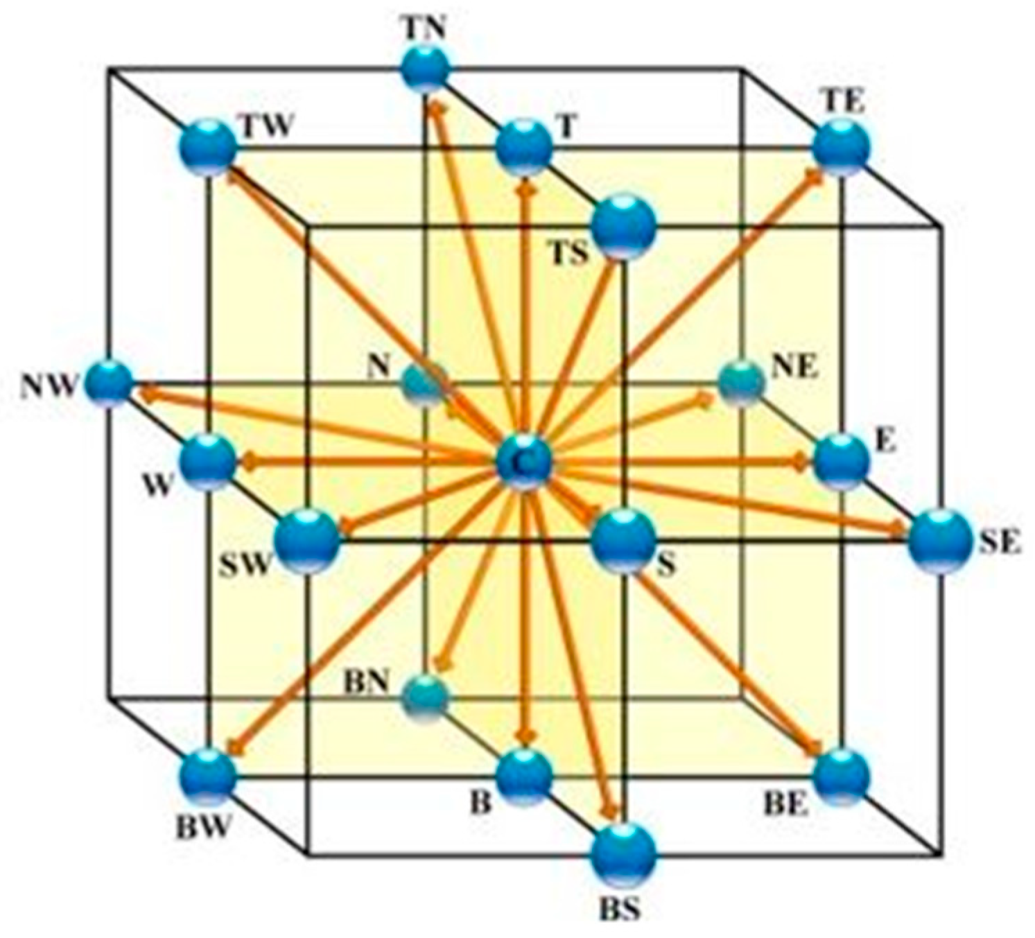
where is the density probability function, is its equilibrium state, is the lattice velocity, and is the dimensionless relaxation time related to viscosity. The equation describes how ‘particles’ of fluid move and interact in a lattice when propagating through prescribed directions, as shown in Figure 1.
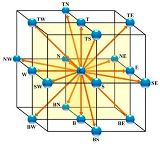
Figure 1.
Discretized velocity directions of liquid ‘particle’ movement among lattice nodes (scheme D3Q19) [13].
The simulation process then consists of two stages: ‘streaming’, where the particles travel, and ‘collisions’, where they interact. Via subsequent mathematical manipulation, this scheme is shown to adhere to macroscopic continuity and Navier–Stokes equations, with which it can be mathematically shown to fully conform without the need for any turbulence models. However, the computational demand for a completely resolved approach is, in most cases, beyond the scope of current hardware. A large eddy simulation (LES) turbulence model is therefore introduced into the discretized Boltzmann equation that accounts for and filters the turbulence at a certain scale with artificial eddy viscosity computed with [12]
where is the empirical Smagorinsky coefficient found between values 0.1 and 0.3, is the grid spacing, and is the shear rate tensor.
The LBM approach to simulating liquid pairs with the Lagrangian discrete element method (DEM) to simulate suspended solid particles as individual points bearing physical properties and traveling through the system. The main drawback of the DEM is that the computational demand grows with the number of particles—i.e., the solid fraction—making it difficult to simulate large or dense systems; this is contrary to the Euler–Euler approach often used with classic finite-volume methods, where both phases are modeled as continua and solid fractions are therefore not a factor for computability. To compensate, an ‘Injection number scale’ option [13] can be utilized, which groups the particles into computational parcels according to a chosen number and thereby simplifies computation. However, the full effects of this feature on accuracy have not yet been well described. Along with its suitability for parallel computing, the DEM also shows great potential for modeling the largely unexplored topic of polydisperse suspensions as each particle can be assigned individual physical properties if needed.
This numerical scheme was shown to be a reliable tool in simulating similar cases to ours, as shown in [14,15,16]. Its direct description of particles in a flow provides an opportunity to revisit established particle interaction models (such as drag force) and examine whether they can support the full potential of this promising method.
1.2. Particle Forces and Drag Force Models
In practical DEM simulations of liquid–solid flows, the resolved fluid grid must in most practical cases be coarser than the particle size, making it impossible to directly determine how the fluid acts upon the particles. The interaction is instead computed as a superposition of forces based on physical laws contributing to Newton’s second law written for particles with interpolated local quantities as inputs [17]
where represents various contact forces, body forces, and interphase forces. Contact forces provide expected interactions between solid bodies in the system and are usually modeled using variations of the Hertz–Mindlin contact model (reviewed, for example, in [17]), where particles exchange translational and rotational inertia through radial and tangential forces and momenta. While these models play an important role, their significance is dimmed in the liquid–solid environment, and contact models are better explored and established. We therefore consider them less worthy of exploration. Body forces such as the gravitational force and buoyancy have sound analytical descriptions. Meanwhile, the interphase forces [18] have posed a considerable challenge in recent research. They include, for example, the drag force , the lift forces of Saffman and Magnus , the virtual mass force and the acceleration history force of Basset , the turbulent dispersion force , and the lubrication forces accounting for the inflow or drainage of liquid as particles separate or come into contact (which may also be categorized as a contact force).
Of these forces, the drag force is both critical and not perfectly understood. The drag force for spherical particles takes the conventional form of [17]
where is the slip velocity (difference in particle and liquid velocity), is the particle diameter, is the liquid density, and is the empirical drag coefficient. This is the vector equation directly used in the DEM method.
The drag coefficient has been reliably modeled for lone particles in steady flow (often denoted in a wider context) with correlations to particle Reynolds number such as those from Schiller [19], Equation (5); DallaValle [20], Equation (6); and more recently Brown and Lawler [21], Equation (7). However, the conditions present in liquid–solid batch mixing are much more complex, reducing the accuracy of these basic correlations. The added complexity lies in at least two added factors: (a) the high micro-turbulence during mixing and (b) the presence of other particles. Many correlations have been published in an attempt to account for these phenomena. Factor (a) is explored, for example, in the works of Brucato [22], Equation (8), and the follow-up works of Khopkar [23], Equation (9); Pinelli [24], Equation (10); and Fajner [25], Equation (11). The common idea is to correct the lone steady particle equations by a factor including the Kolmogoroff scale in relation to the particle size as . Factor (b) is explored, for example, in the works of Di Felice (12) [26] and the follow-up work by Rong et al. [27], Equation (13), or by Gidaspow [28], Equation (14) (a combination of two older models of Ergun [29] and Wen Yu [30]). These authors correct the lone steady particle models through dependency on the liquid fraction or particle fraction (where ). Most recent contribution of this kind was made by Wang et al. [31], Equation (15), with the exception that it is not based on an existing lone steady particle model. This dichotomy in modeling drag force in mixing was also noticed and studied by the authors of [32], who concluded that each of the approaches gave better results in different parts of their tank. The mentioned models are summarized in Table 1, and a broader selection of available models can be found in [31].

Table 1.
Selection of common drag force models sorted by approach.
Notably, of the listed models, Equations (7) and (13) are implemented in M-Star CFD as ‘Free Particle’ and ‘Packed bed’ DEM options, respectively [13], and Equation (14) is used for modeling the Euler–Euler heterogeneous flow in Ansys Fluent [33].
In addition to the large number of available drag force models, uncertainties lie in their correct implementation. For example, Equations (8)–(11) were correlated experimentally with mean calculated from shaft work. However, CFD software allows for the use of local numerical values, which better describe local turbulent conditions but might contradict the model’s nature. These issues were tackled in [32]. Similar disputes can arise when considering the particle Reynolds number and whether it should be multiplied by , which is also often surprisingly unclear (as seen, for example, in the model presented in [27] and its applications, for example, [13]). Another point to consider is that some definitions of drag forces may intentionally or unintentionally encompass effects from other interphase forces in their derivation. For example, Equation (15) was derived to be taken as the sole interphase force in mixing applications, and equations from the (a) family may cover the similar influence of eddies as the turbulent dispersion force .
This brief review shows the lack of established procedures for choosing and implementing a drag force model into a numerical scheme; this may, however, be amended via a broader effort to validate these models on different cases and numerical setups.
1.3. Validation of Drag Force Models on Engineering Cases
Many works have therefore focused on comparing the agreement of these models with various experiments, both in the field of liquid–solid mixing and outside of it. Reference [27] reported differences ranging from to for the case of flow through a steady packed bed (the exponent of the voidage function is compared). The local solid fraction distribution results from the numerical studies of [31,34] showed large local deviations from experiments in cases of mixed batches. Reference [32] compared several drag force models in the case of an axially mixed tank, with larger errors found near the top of the tank and in the impeller area. The authors of [35] reported that no drag force model fits their experimental data particularly well in the case of a spouted bed, which shares physical similarities with the case of a mixed tank. Preliminary inhouse numerical trials gave similarly unsatisfactory results for all tested drag force models. Notably, we were unable to acquire any suitable results with the new model Equation (15) of Wang et al. [31] in our numerical environment. Generally, it appears that while the current well established drag force models work sufficiently well, there is still room for improvement, which is critical to explore due to the described importance of drag force.
1.4. Off-Bottom Suspension Flow Patterns
Since precisely reproducing the distribution is often troublesome, a more general indirect criterion for comparison is explored—the flow behavior surrounding an off-bottom suspension in a mixed batch. The most well-known approach to describing the off-bottom suspension is the Zwietering criterion [36] with the just-suspended impeller speed given by
Which predicts the just-suspended impeller speed , defined as the state when no particle on the tank bottom remains stationary for longer than 1–2 s. Many improvements and alternatives to predicting have been published. For example, Rieger’s approach of dimensionless correlations for the modified Froude number [37,38] and, more recently, the notable GMB equation [39].
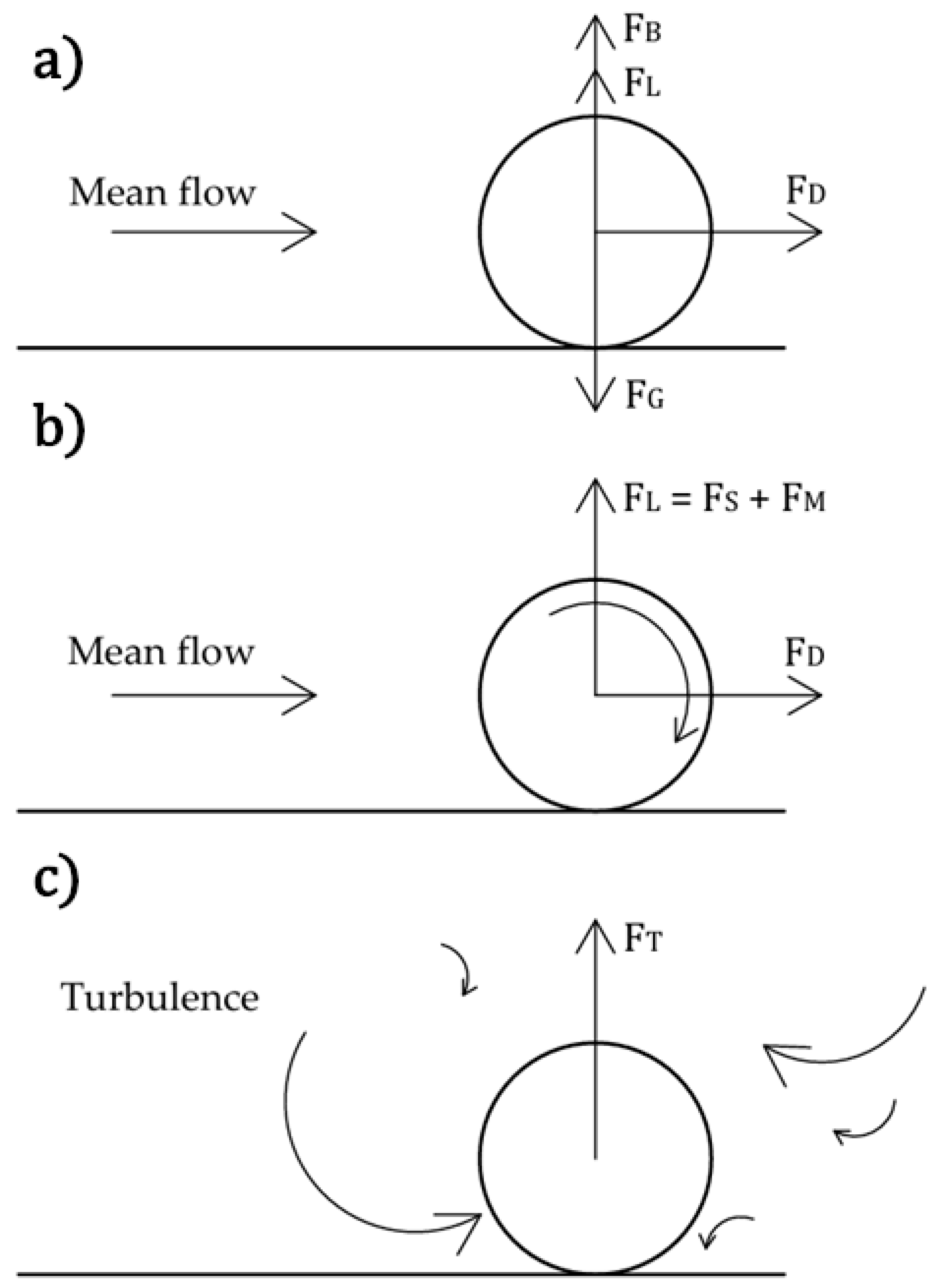
Many works have also explored the fundamental local physics causing the particle to lift; notably, [2], which distinguished two different mechanisms for the off-bottom suspension of particles—one via mean flow associated forces and and the other through turbulence associated force (Figure 2). Lift caused by eddies of a similar scale to the particle is also the basis for the GMB critical impeller speed correlation [39]. The size and time scale of eddies for particle off-bottom suspension were studied and precisely determined in [16].
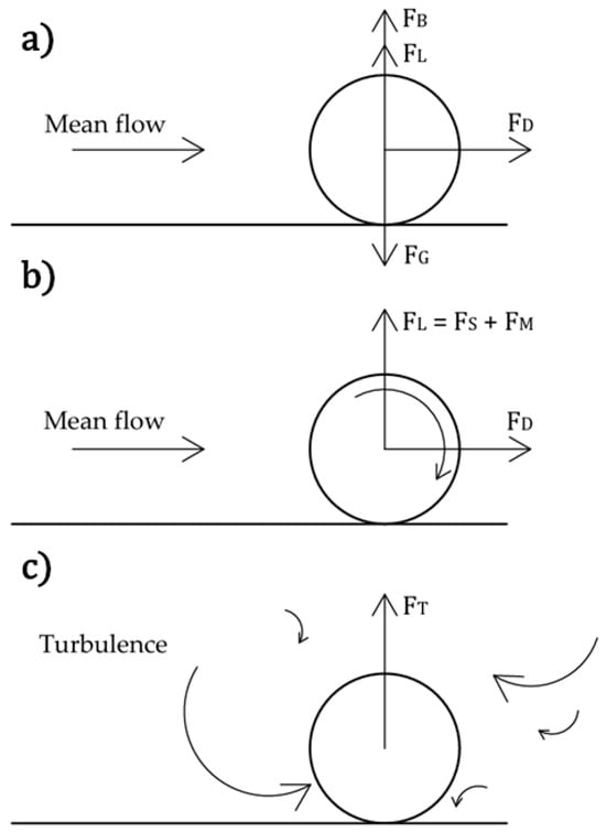
Figure 2.
Mechanisms of off-bottom suspension: (a) all forces; (b) forces caused by mean flow; (c) forces caused by eddies [2].
Considering the above, it may seem that the drag force does not play a significant role in the off-bottom suspension of particles. This is, however, only true when considering the very initial lift of each particle and not the following entrainment into the main flow, not to mention the effect of the drag force on the overall flow behavior and the following influence on the initially acting lift forces. We would therefore like to stress the difference between this narrow fundamental definition of the particle off-bottom suspension and the more general studies of near-off-bottom suspension flow patterns that will be studied further in this work, where the drag force is essential and which could prove useful for comparison of drag force models, as will be shown later.
Note that the off-bottom suspension is achieved gradually, with a growing percentage of sedimented particles joining the mixing process until is reached. Rieger [37] theoretically described the flow patterns present on the bottom of mixed batches (Figure 3) that form when reaching the suspension with the axial impeller, best observed in a flat-bottomed tank. At these impeller speeds, the just-suspended particles described in Figure 3 form the interface between the main flow and the still sedimented areas; as a particle is lifted from the tank bottom or inclined patches of sedimented particles, it is entrained by the mean flow dominated by drag force. Particles dragged radially outward by the mean flow through the well-mixed ring on the bottom encounter the outer sedimented patch, which was observed to serve as a sort of ‘ramp’ for further upward entrainment of particles. The sedimented patches then serve as an indirect indicator of the flow behavior, as shown in inspection analysis where the inner and outer radii and of the ring washed out in the sedimented layer follow the dependence [40]
where is the modified Froude number (dimensionless form of the critical impeller speed) and the Reynolds mixing number [40]
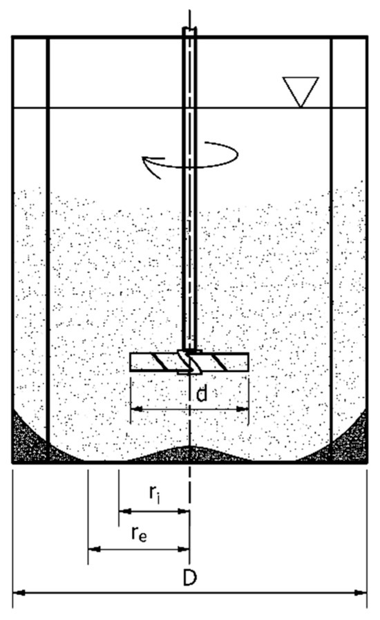
Figure 3.
A diagram of expected behavior of an axially mixed batch with ‘relatively small’ particles when reaching an off-bottom suspension [40].
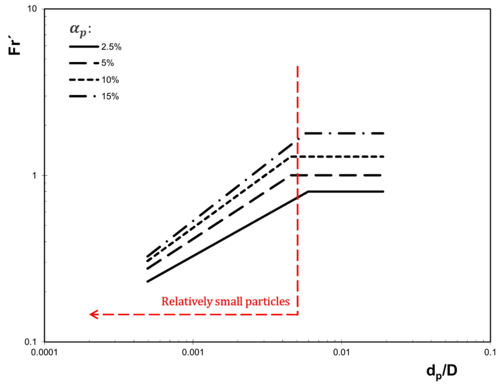
The most important trait is that the well-mixed ring in settled particles slowly grows with the impeller speed until a full off-bottom suspension is reached. This mechanism is present for ‘relatively small’ particles in the sense of Figure 4, described using the ratio of particle size to tank diameter.
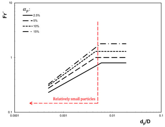
Figure 4.
Dependency of modified Froude number on relative particle size and particle fraction with highlighted area of ‘relatively small’ particles [38].
Naturally, this process also occurs inversely: when lowering the impeller speed from higher than critical values, the particles gradually settle from the flow into the sedimented patches. Although there was no significant difference observed in critical impeller speeds whether reached from below or above for low solid fractions [37], this notion helps us to further stress the previously mentioned difference between approaches to particle lift since in the case of decreasing impeller speed, it can be assumed that a particle will join the sedimented patch when it loses sufficient drag from the mean flow above.
Focus on impeller speeds below just off-bottom suspension was further encouraged by the authors of [6], who pointed out that in industry, operation below is often sufficient yet has not been sufficiently studied in the literature.
Jirout et al. [41] later pointed out the subjectivity of the Zwietering criterion and related visual reads and introduced electrochemical probes to precisely and consistently map the presence of stationary particles pointwise across the tank bottom. They also mapped the broadening ring using this approach. Via changes in current, the electrochemical probes detect hydrodynamic fluctuations that seize when stationary particles are present and covering the probes. This removes the role of the observer from the process and gives reliable and repeatable results.
Similarly, the pressure gauge method developed in [42] measures the local fraction of particles suspended via an increase in pressure on the vessel bottom that occurs as particles are lifted. The apparent density of the liquid increases due to solid presence, resulting in a steeper hydrostatic gradient and greater pressure maximum on the tank bottom. This method has the advantage that the measured quantity (pressure) is more closely related to the off-bottom suspension phenomenon itself, making it suitable for comparative experiments and simulations. Both methods [41,42] have the disadvantage of using mediating local quantities, while the original visual method [37] accounts for the entire tank bottom continually and directly and does not require any alterations of the tank.
The authors of [43] mention in their article a method of photographing particles on the tank bottom and using image analysis to compute the ratio of sedimented patches to well-mixed areas to find . This approach is similar to that used in further presented experiments, but it does not follow the border and therefore does not build on Rieger’s work.
Reference [5] points out that the comparison is difficult to apply since the Zwietering criterion cannot easily be implemented in a numerical environment. However, they recorded a very close match by comparing pressure gauge method [42] readings to numerical pressure values. Other methods for establishing the suspension in simulations were found to be unsatisfactory.
2. Experimental and Numerical Setup and Methods
In this work, we decided to conduct our own set of experiments and compare the results with LBM simulation results using the DEM particle model with various drag force descriptions. We chose to compare the Brown and Lawler model [21], Equation (7); the Rong model [27], Equation (13); and the Gidaspow [28] model, Equation (14), as they appear to be the most often used models in mixing based on our research. This comparison was conducted using Rieger’s description of the gradual off-bottom suspension (Equations (17) and (18)) as an indirect measure of the system’s behavior. The well-mixed ring dimensions and from Figure 3 were compared at various impeller speeds below . In further sections, the details of experimental method, the numerical approach and, finally, the new tools used for the comparison are discussed.
2.1. Setup of Experiment
A transparent, flat-bottomed tank (Figure 5a) with and four baffles of width was filled with a mixture of tap water ( and ) and spherical glass particles ( and ) to various volume fractions and mixed with a down-pumping 6-blade pitched blade turbine (PBT) with using blades of width and thickness of 1 mm inclined under 45° (Figure 5b). The impeller clearance was set to . The experiments were conducted at a room temperature of 20 °C. This setup was chosen so that particles were relatively small, according to Rieger’s definition in Figure 4, but large enough not to exceed the computational limitations of the DEM method when achieving the desired solid fraction. A camera was installed below the tank to photograph the distribution of particles on the bottom, and an LED light was used to illuminate the tank from above when needed.
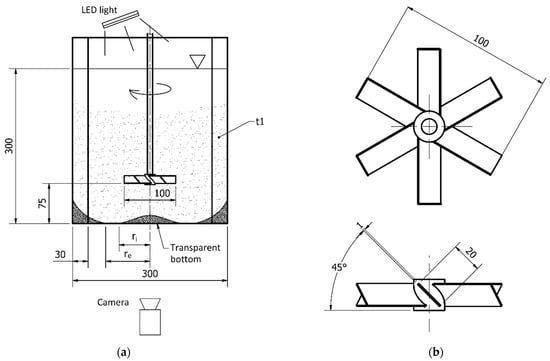
Figure 5.
(a) Experimental setup (dimensions in mm); (b) schematic of impeller used (dimensions in mm).
The solid volume fractions of particles were prepared via weighing. The critical impeller speed was found for each loading, and the impeller speeds to be measured were then chosen below these values at regular intervals of 40 min−1. Care was taken to minimize the possible negative effects from the resonance of the impeller speed and image capturing frequency (in case the patterns showed time-periodic behavior). Approximate homogeneity was first reached to further separate the influence of drag from other previously discussed effects related to the off-bottom suspension of particles, and then each prescribed impeller speed was approached from above, meaning the measured shapes emerged from particles settling with a decrease in the impeller speed. This procedure should help to alleviate the influence of particle–particle interactions and the initial lift forces discussed in Figure 2. We assume that the measured patterns are composed of particles that can no longer be held in the main flow circulation by the drag force, making them an indirect indicator of the drag force’s influence.
The camera took 30 photos for each impeller speed every 2 s for a total duration of 60 s. For sets , an LED light was used to shine through the particles. The shapes in the sedimented layer were otherwise indistinguishable. All measured states are compiled in Table 2. The impeller speed was set with a maximum error of . While all combinations of impeller speeds and solid fractions were measured, not all could be analyzed via our method; at low impeller speeds and high solid loadings, no patterns were identifiable in the dense settled layer. Contrarily, when nearing just off-bottom suspension, the patterns become too volatile to be identified even after averaging.
Table 2.
Overview of measured and evaluated cases.
2.2. Setup of CFD Simulation
The experimental setup was reproduced in the LBM software M-Star, version 3.10.32. Since commercial software was used, the underlying numerical structure is not extensively discussed. The nuances of the solver can be reviewed in the official documentation [13].
Due to the large number of DEM particles required to satisfy Rieger’s conditions (Figure 4), many approximations must be undertaken for the setup to be computable on contemporary machines, making the presented simulations less rigorous than those reviewed. Many factors proven to influence the off-bottom suspension are simplified, which will be further discussed in following sections (e.g., the simplified contact model, neglected particle rotation, and implemented particle grouping). This, however, presents the opportunity to examine how simulations run in engineering practice compared to reality and how the drag force model influences the flow patterns in such conditions.
2.2.1. Continuum Model
A large eddy simulation (LES) LB transient single-phase approach filtered using the Smagorinsky approach was chosen for the liquid with a Smagorinsky coefficient , supported by the review in [15]. The chosen lattice type was ‘D3Q19’, with 19 possible velocity directions. A rectangular uniform mesh was adapted with 250 lattice cells across the tank diameter, which corresponds to cell size of . Reference [13] shows that this is sufficient to safely reach grid independence in the sense of shaft power input for geometry closely similar to ours. On the bottom and walls, grid-aligned boundary conditions enforce no-slip conditions by reflecting the liquid particles, while the surface has the no-shear condition. The simulation timestep was chosen as seconds to accommodate stable DEM particle tracking across all impeller speeds considering the selected contact model. Convergence was checked via the LB density value, which represents how well the macroscopic values are preserved.
The LB method reproduces RANS Navier–Stokes equations not involving the non-negligible solid fraction correction. The solid’s volume is instead accounted for by modifying the continuum’s dynamic viscosity with Euler’s equation according to [44]
where is the dynamic viscosity, is the model’s constant, and is the close sphere packing solid fraction. is then further increased using the Smagorinsky viscosity from Equation (2). Together with this, the liquid receives a reaction force from the particles from two-way coupling. The movement of the impeller is simulated via the immersed boundary method [3].
2.2.2. DEM Model
The particles were smaller than the lattice resolution, and their behavior was dictated strictly by the sub-grid particle force models. They were two-way coupled with the liquid, receiving local physical values extrapolated from nearby lattice points. Since the computational demand of simulating all particles rigorously would be quite high at a solid fraction , the particles were parceled into groups of 10 by the software’s ‘injection down sampling’ option for all cases—this is considered the largest stray from the proper description. The ‘Third law number scaling exponent’ of this option was left at the recommended 0.5. The rotation of particles was neglected. The interactions between the particles and walls, particles and impeller, and among particles themselves were dictated by M-Star’s implementation of the Herz contact model named ‘Bounce Simple’ or ‘Hertz Simple’, which prescribes the following collision properties [13] summarized in Table 3:
Table 3.
Summary of Hertz’s contact model parameters used in simulation.
These parameters are prescribed to prevent solid overlaps ( and secure numerical stability without requiring an unachievably small timestep but do not account for the actual contact properties of the involved materials, which were shown to also affect the system behavior. We accept this as another approximation.
Gravitational, buoyant, and drag forces were considered from the other forces acting on particles. Three drag force models were tested: Brown and Lawler [21], Equation (7); Rong [27], Equation (13); and the Gidaspow [28] model, Equation (14), as a user-defined function. Their precise formulations can be reviewed in Table 1.
2.2.3. Simulation Procedure
The required solid load was added through an arbitrary volume over the bottom part of the tank. During the first 10 s of the simulation, the impeller was set to a high speed of near homogeneity and then lowered to the required impeller speed, corresponding to the experiment. Then, the particle distribution data were captured every 2 s for an interval of 60 s, giving us 30 images for each impeller speed.
2.3. Visual Comparison Method
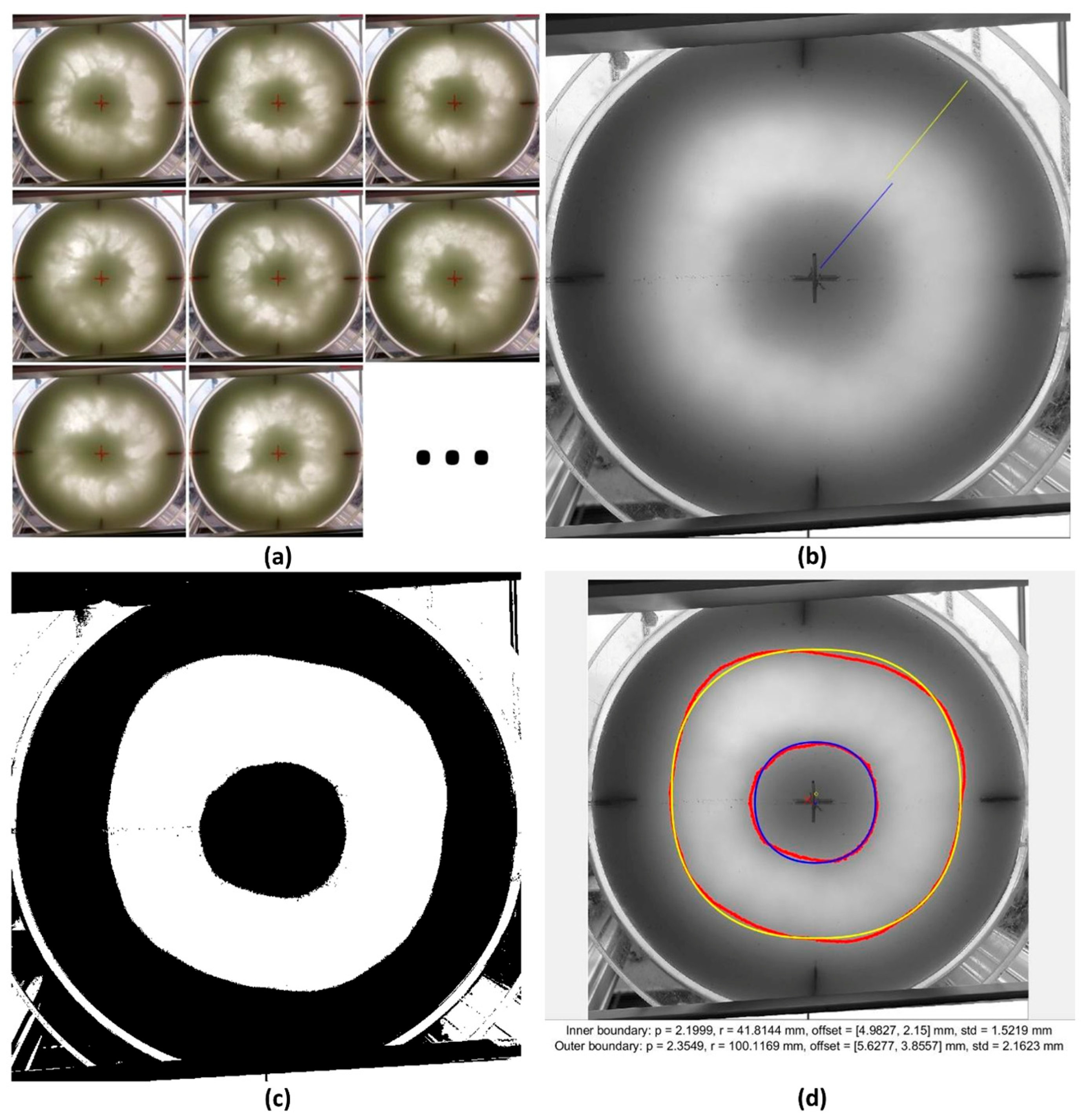
The dimensions and were extracted from both the experimental and numerical results and compared for evaluation. The high uncertainty inherent to indirect visual methods was reduced by using a computer image processing tool written in MATLAB R2023b [45].
To obtain data equivalent to experimental photos from the CFD simulation, the most straightforward method was chosen—2D views of the vessel bottom were rendered in the simulation’s post-processing. The DEM particles are represented as black points. Thus, the analogy to Zwietering’s and Rieger’s original visual approaches holds. Similarly to the experiments, emerging patterns were in many cases indistinguishable. It was found that lowering the opacity of the particles (black points) in the rendered view as an alternative to shining through them with an LED light as in the experiments helps to reveal the shapes. Lowering the opacity causes the otherwise fully opaque black points to become transparent and reveal other particles behind them, turning the height of sedimented patch to a white-black gradient when viewed on a white background. Visual conditions in which images were captured both in the experiment and simulation are given in Table 4 for all cases. These visual conditions were chosen via inspection, so all images across various impeller speeds were analyzable and visually similar overall. It is obvious, however, that in our implementation of the visual method, these conditions affect the results and should be more carefully calibrated in the future (this is further discussed in Section Sensitivity Tests of the Visual Comparison Method).
Table 4.
Visual conditions used to make shapes visible when capturing data for various measured volume fractions.
Both numerical and experimental images were processed using the same computer image processing tool. It is important to note that part of the visual method’s subjectivity comes from the fact that the shapes’ dimensions can change with time and the azimuthal direction. The new tool accounts for both these factors and compares data consistently. The method’s structure is visualized in Figure 6. Its major steps are described in greater detail in further sections. The comparison method is viable for relatively small particles in the sense of Figure 4, leading to the reliable emergence of patterns, and on volume solid fractions ranging from approximately to , resulting in discernable patterns.
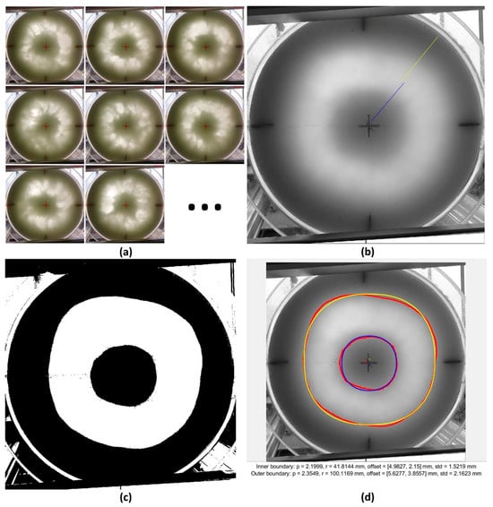
Figure 6.
Simplified workflow chart of data processing: (a) a sample of images of tank bottom; (b) average of images; (c) binarized image with border; (d) image analysis result. Blue—inner interface; yellow—outer interface.
2.3.1. Time Averaging of Pictures
2.3.2. Border Detection
Next, borders between the well-mixed ring and fully settled particles needed to be established—this is a question of finding a brightness threshold in the gradient of Figure 6b and turning it into a sharp edge in Figure 6c. This substitutes the subjective judgement of the observer of where the border lies if the fluctuating pattern is observed firsthand. There is still uncertainty in where the line should be drawn; the threshold, however, is precisely numerically defined and can be controlled and kept consistent. It was decided to find the threshold naturally from the arithmetic average of brightness values of a bright point in the middle of the well-mixed ring and dark point from the sedimented patch separately for the inner and outer boundaries (as illustrated by lines in Figure 6b). This choice will be further discussed in Section Sensitivity Tests of the Visual Comparison Method. These values were then used as the threshold values for the ‘imbinarize’ function in MATLAB [45], which finds both inner and outer interfaces using Otsu’s method [46]. Essentially, the gradients are each cut halfway through. If the gradients are not sufficiently pronounced (e.g., the sedimented layer is too thick, or the mixture is too diluted), the method fails at this stage.
2.3.3. Fitting the Shapes
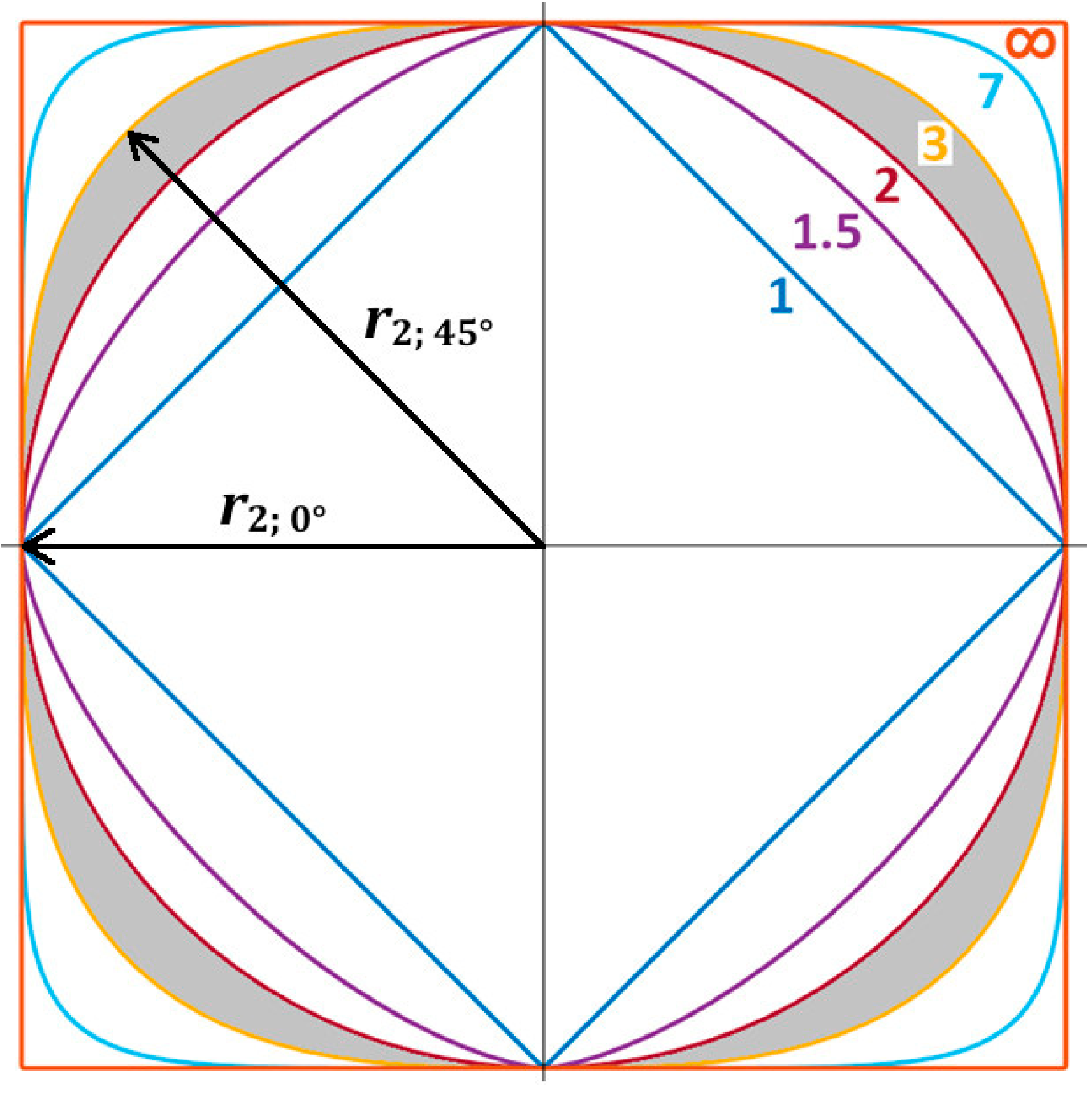
In Figure 6b,c, it can be noticed that the averaged shapes do not appear as perfect circles. The variation in the azimuthal direction can be attributed to the presence of four orthogonally spaced baffles (the most common setup in mixing) that bestow a certain ‘rectangularity’ upon the otherwise circularly symmetrical case. This means that an observer would read a different measure of the shape in the baffle plane and in the plane midway between baffles. To account for this, the shapes were described not with Euclidean circles, but with -norm circles that capture the flattening effect of baffles quite well. Such a shape can then be described with the same value everywhere, together with an exponent accounting for the ‘rectangularity’. The -norm defines the distance between arbitrary points and in -dimensional space as [47]
Based on this general formula, the -norm circle in two-dimensional space appears as (essentially a generalized Pythagorean theorem)
The universal can be transformed back into Euclidean space via the following relations in directions of interest
| Baffle plane: | (24) | |
| Mid-baffle plane: | (25) |
Examples of -norm ‘circles’ are shown in Figure 7. The axis are expected to align with the baffle planes, as baffles are the cause of deformation. As an example, when working with -norms, the yellow circle has the same radius everywhere but different Euclidean dimensions in the baffle plane and (note that the dimension in baffle plane is always conserved). This varies the actual measures by from the baffle plane to the mid-baffle plane by 12.2%.
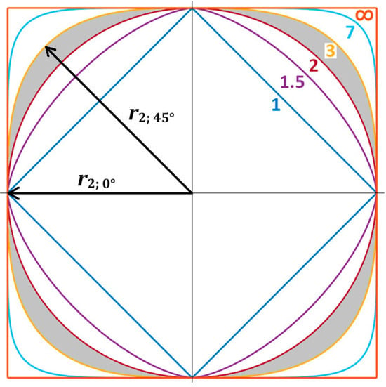
Figure 7.
Circles with p-norms using different p exponents (1, 1.5, 2, 3, 7, ∞). Baffle and mid-baffle Euclidean dimensions are shown on the p = 3 unit circle. The gray shaded area shows the expected region for most of our data.
This parameter is certainly a function of baffle geometry and serves to quantify the effect of baffles on the system. A perfectly symmetrical unbaffled system would be expected to have ; standard baffles (0.1D) are shown in this work to compress the shape—usually to and baffles of larger proportions are expected to increase the values even further.
A regression algorithm was used to approximate the borders in Figure 6c with -norm circles to obtain the final results in Figure 6d. Equation (26) was transformed into polar coordinates in the -norm
A sum of squared differences of these coordinates to all points of the previously found threshold was taken, and the sum was then minimized by varying and values. This optimization task was performed using the ‘fminsearch’ function in MATLAB [45] using the simplex search method [48]. A regular -norm shape was thus found that best approximates the entire threshold with just two values.
In-between the previously described major steps, the script also performed minor tasks, such as finding the geometrical center of the vessel and comparing it to the center of the set of points describing the threshold (useful for eliminating the influence of asymmetries in the system, such as an off-center impeller) or acquiring real dimensions by scaling to the known vessel diameter as a reference.
The radii of the inner and outer well-mixed area boundaries were found for each measured impeller speed with their corresponding exponents and standard deviations.
3. Results
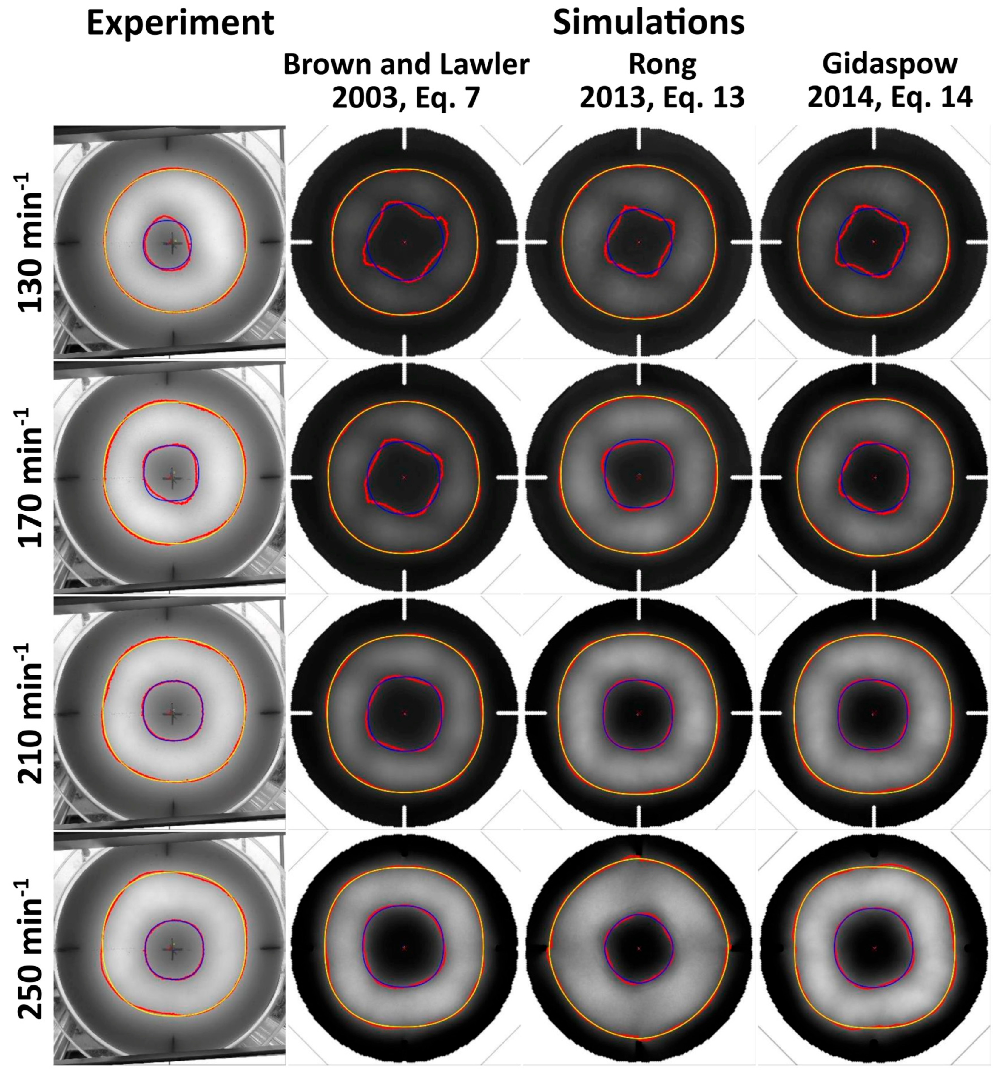
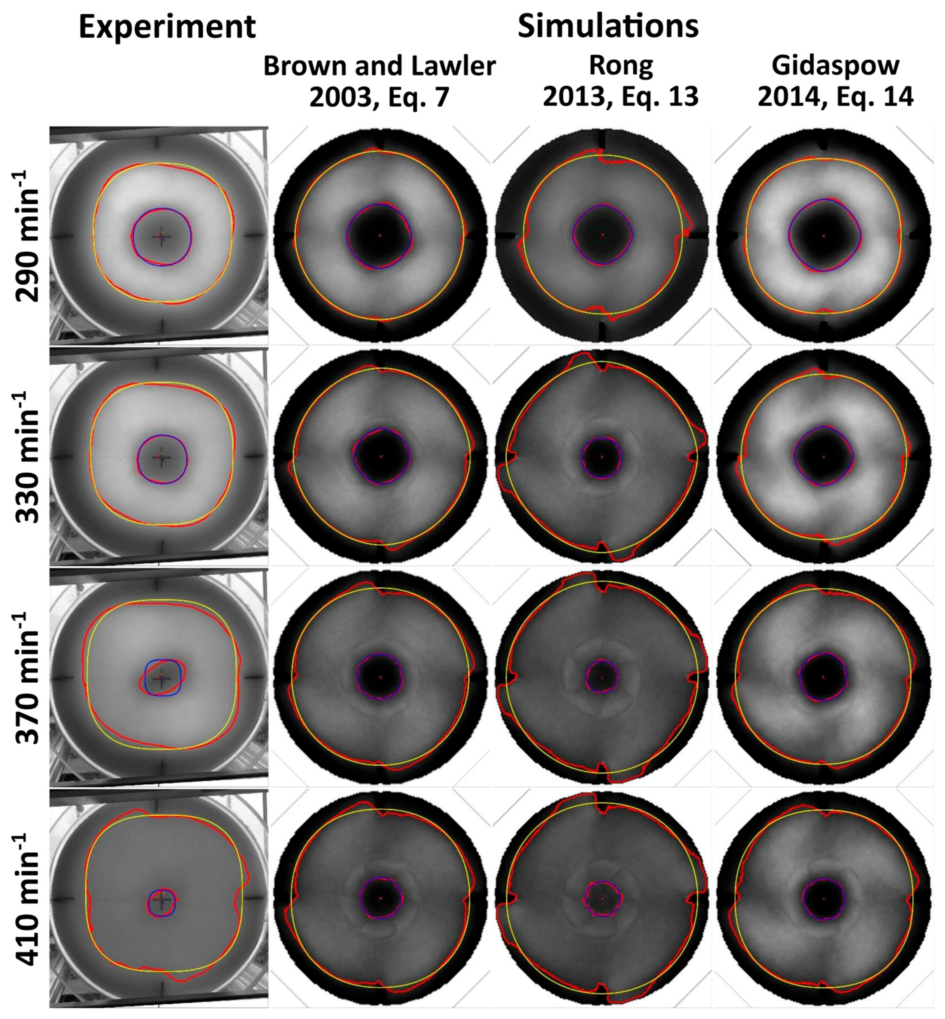
A summary of the main results is presented. We chose to list the results in ascending order of impeller speeds, despite having captured them in reverse order. In Figure 8 and Figure 9, full, resolved visuals showing the experimental and numerical results are presented for the mean solid fraction of , comparing the chosen drag force models Brown and Lawler [21], Equation (7); Rong [27], Equation (13); and Gidaspow [28], Equation (14), with the experimental results (visual results for other solid fractions are left out for brevity as they show very similar behavior). Note that the baffles were darkened for higher impeller speeds in the simulation results to avoid interference when detecting the outer border.
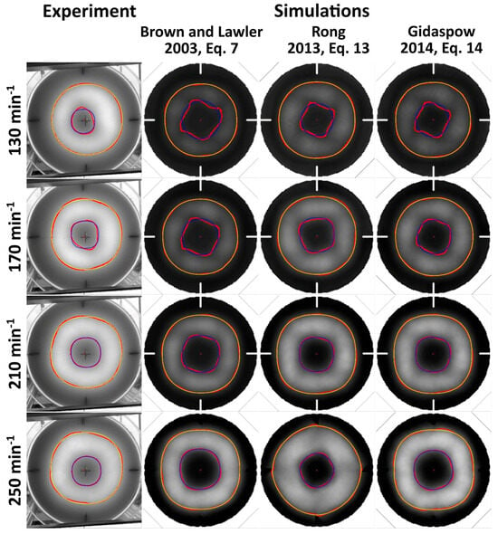
Figure 8.
Comparison of visual results from experiment to renderings of numerical simulations for 5% volume (n = 130 to 250 min−1) with drag force models [21,27,28]. Blue—inner interface; yellow—outer interface.
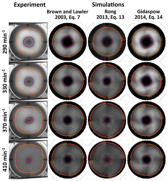
Figure 9.
Comparison of visual results from experiment to renderings of numerical simulations for 5% volume (n = 290 to 410 min−1) with drag force models [21,27,28]. Blue—inner interface; yellow—outer interface.
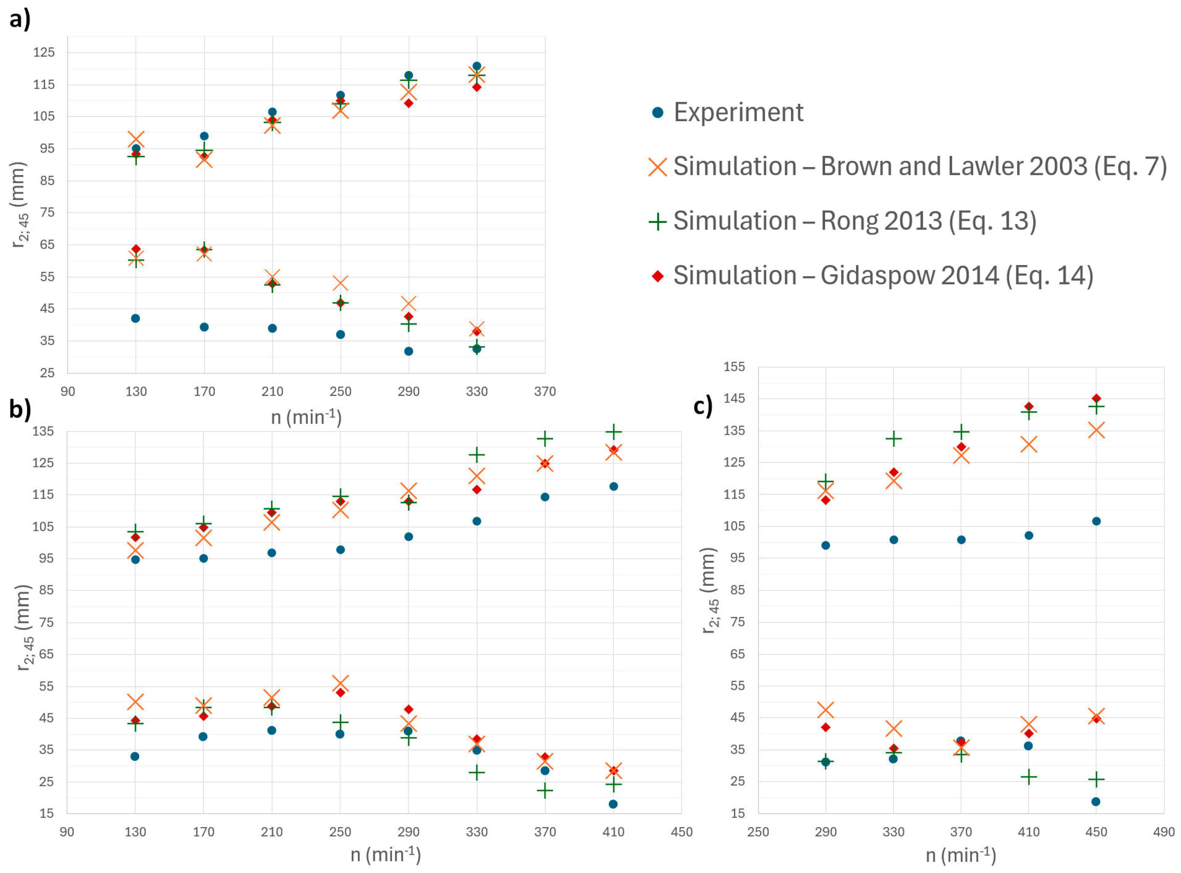
In Figure 10, the quantitative results for all measured mean solid fractions are presented. The measure (midway between baffles) of the rings (Equation (25)) was chosen as the parameter for comparison, as was the one measured in published experiments [41]. The method yields expected results as the measures of the ring tend to widen with the increase in impeller speed and particles being mixed. Figure 10 further shows regions where this does not hold (lower impeller speeds for 5% and 10% solid fractions at the inner interface, where increases). This is due to increasing fluctuations of the interface that ‘smear’ the central settled patch and make it seemingly grow with the impeller speed.
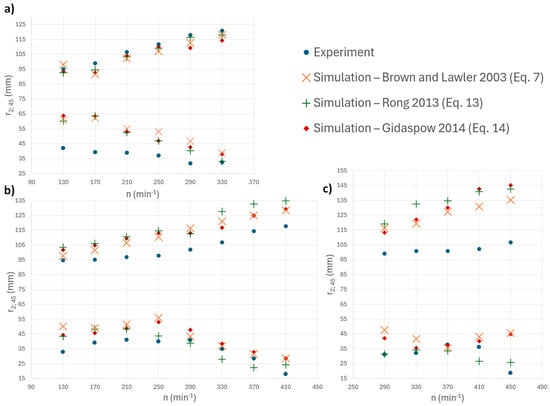
Figure 10.
Overview of inner and outer radii of the well-mixed rings when approaching the just off-bottom suspension in mid-baffle plane for (a) 2.5%; (b) 5% and (c) 10% solid volume fractions (impeller speeds where pattern recognition failed were not considered). Simulations use drag force models [21,27,28].
In Table 5, the relative differences in of the simulation results from the experimental values were for each case averaged from all impeller speed measurements to roughly quantify how well simulations replicate the experiment. The averages of relative differences were taken separately for the inner radius, outer radius and for both together in total. The differences were taken in absolute values. Cases where simulated values exceeded or underestimated the experimental values over all measured impeller speeds are marked with (+) and (−), respectively. Variable cases are left unmarked.
Table 5.
Overview of relative differences between experiment and simulation for tested drag force models (averaged over all measured impeller speeds).
From Figure 10 and Table 5, it can be inferred that the Rong model [27], Equation (13), reproduced the experiments the most consistently, especially on the inner interface. It, however, overestimates the outer interface at higher impeller speeds with 5% and 10% solid fractions. This could be because it was developed for static bed and does not handle the fiercer conditions at higher impeller speeds well; hence, it is surpassed by the Brown and Lawler model [21], Equation (7), developed for lone particles. The Gidaspow model [28], Equation (14), fares quite well despite being adapted from an Euler–Euler scheme. Its inclusion of the solid fraction seems to be more conservative compared to the model of Rong [27], Equation (13), as it remains closer to the lone particle described by Brown and Lawler [21], Equation (7).
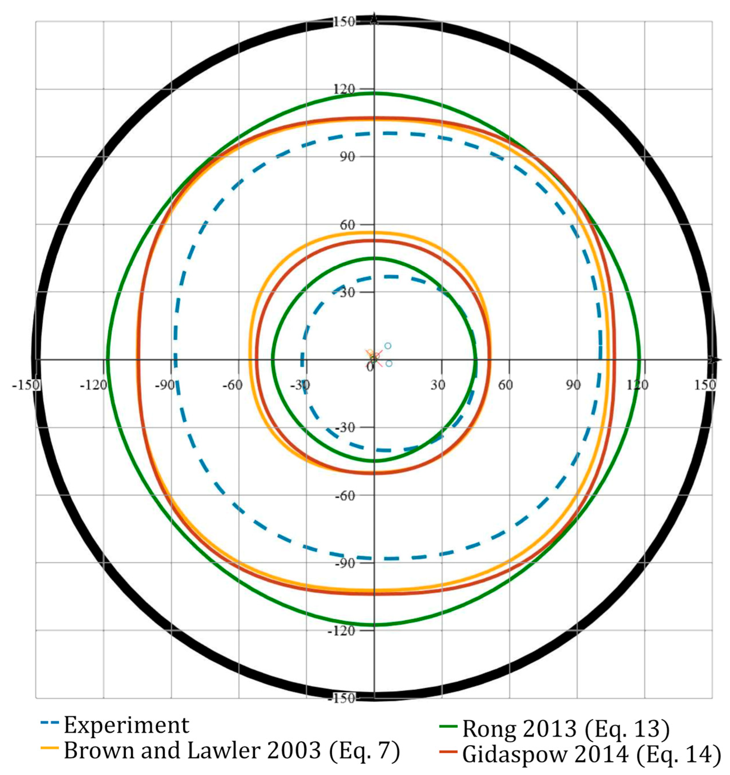
Alternatively, the new method allows us to compare the curves graphically, to review their differences directly in greater detail. Here, it is also possible to include their offset from the center, if one is detected. Curves reconstructed from and and values and their individual center coordinates are compared in Figure 11 for the 5% solid fraction and an impeller speed of 250 as examples.
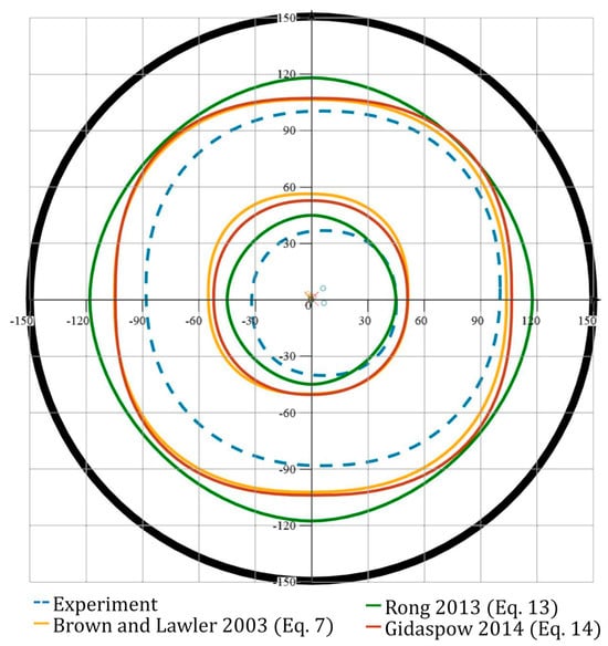
Figure 11.
Direct graphical comparison of -norm circles from experiment and different drag force model [21,27,28] simulations.
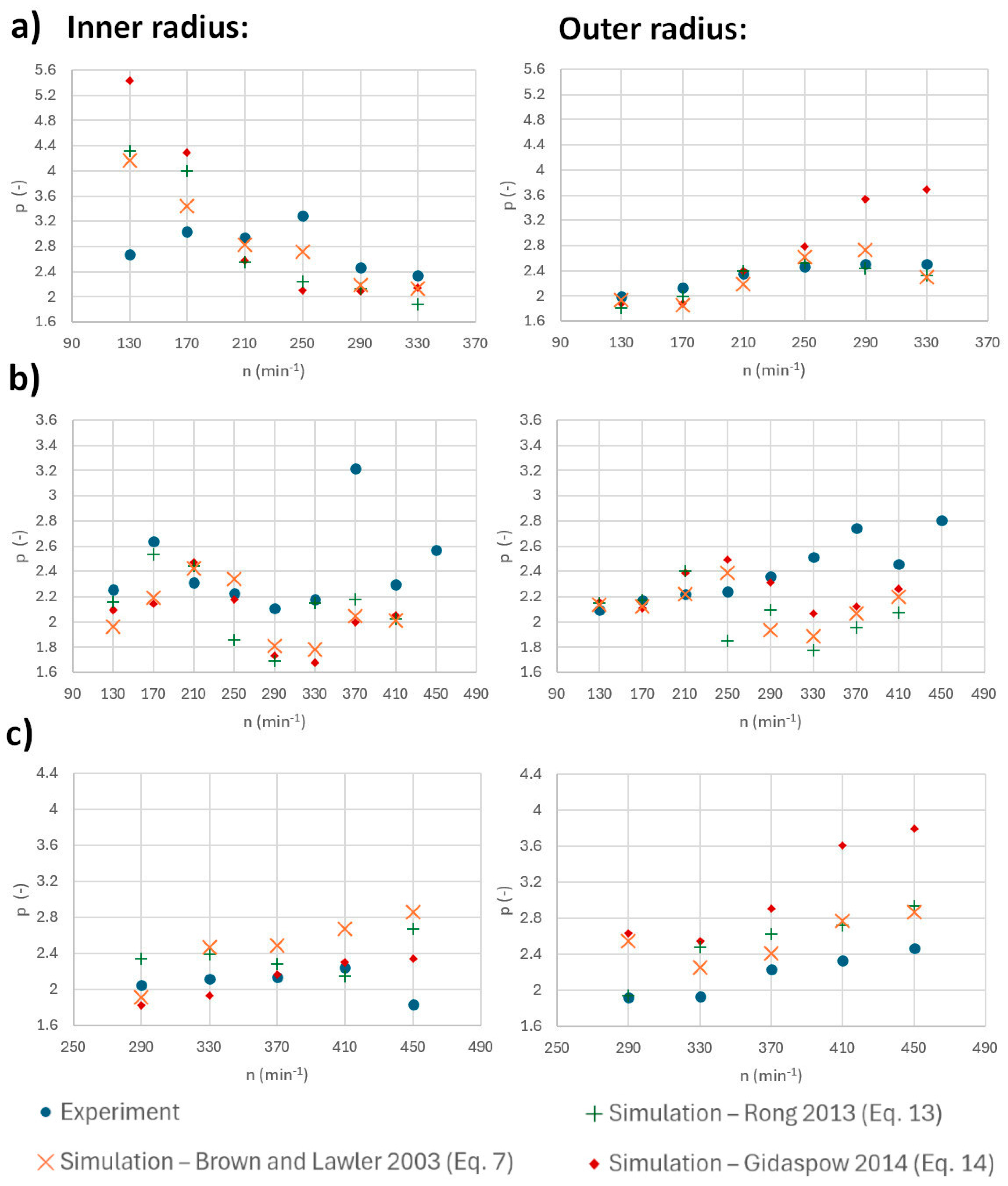
Next, the affiliated parameters are presented. Firstly, in Figure 12, the behavior of the parameter describing the deformation of the circles for 2.5%, 5%, and 10% solid fractions is shown. While the values behaved more erratically, it can be seen that the outer values tended to grow with the impeller speed as the ring broadened and the outer interface approached the baffles, increasingly deforming the circle. Unexpected drops of below 2 were detected in some simulation cases, for example, at the medium impeller speed with a 5% solid fraction. This means that the mixed region drew closer to the edge at the baffle planes (see Rong model [27], Equation (13), in Figure 11). This sudden drop further seems to be consistent with the experiment on the inner interface, despite the experiment not dropping below 2.
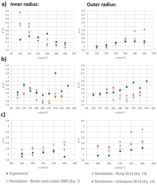
Figure 12.
Overview of exponents for inner and outer radii when approaching the just off-bottom suspension for (a) 2.5% volume solid fraction; (b) 5% volume solid fraction and (c) 10% volume solid fraction. Simulations use drag force models [21,27,28].
The last quantity recorded in the visual analysis was the standard deviation calculated between the regression function and the actual interface, giving an idea of the error stemming from the geometric assumption imposed on the actual shapes. This value held between 1 to 3 mm in most cases, increasing up to 4 to 8 mm when the outer interface approached the baffles at high impeller speeds, where the particles tended to wrap around the baffles unevenly.
Sensitivity Tests of the Visual Comparison Method
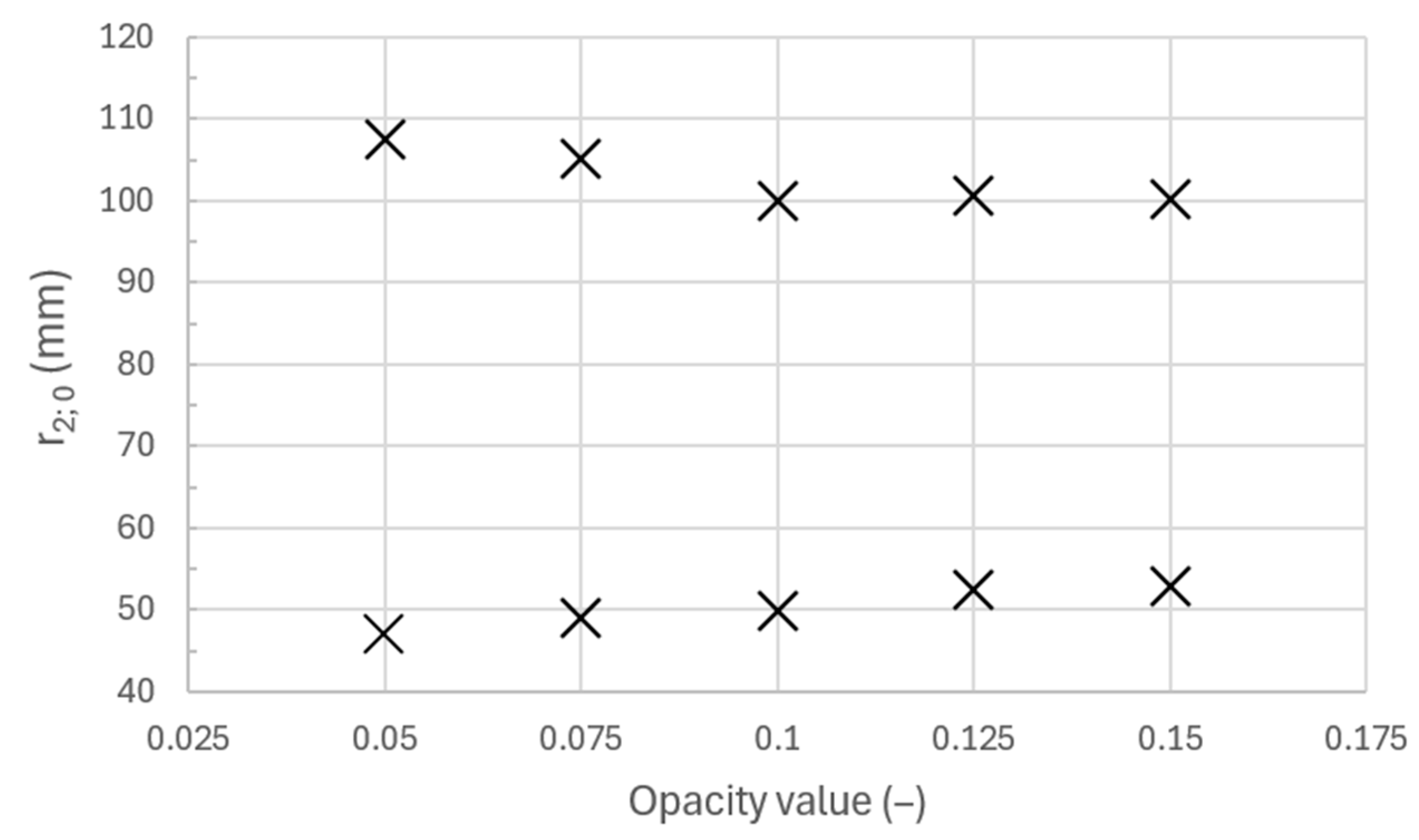
As described in Section 2.3., the visual conditions (i.e., the lighting in the experiment and particle opacity in the simulation) were chosen to match approximately. This choice affected the results, however. The findings presented in Figure 13 in the case of a 5% solid fraction, where the opacity of 0.1 was earlier chosen for the comparison with the experimental results, were studied. It is apparent that the possible error, while not critical in the context of mixing, cannot be neglected when comparing simulation results to those of experiments.
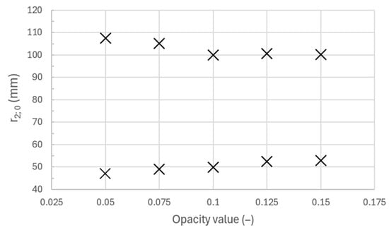
Figure 13.
Sensitivity of numerical simulation results to opacity settings for the visual method.
Based on this, a visual calibration procedure should be developed in the future to determine which opacity best replicates the experimental lighting conditions to prevent possible error from dependency presented in Figure 13.
Lastly, we discuss the sensitivity to the threshold choice. As described in Section 2.3.2, the gradual change in brightness from patches of settled particles to the well-mixed ring was reduced to sharp borders by taking the simple averages of brightness values from both areas (Figure 6b). However, if the weighted average is used instead, the gradient can be cut at specific ratios other than halfway through. This quantifies another aspect of the observer’s subjectivity in the original method—a higher weight coefficient given to the bright value means that the border is found nearer to the well-mixed area, corresponding to a strict observer who measures peaks of the fluctuating particle layer; on the other hand, a higher weight coefficient given to the dark value pushes the border deeper toward the settled particles, corresponding to a benevolent observer, who considers even slight movement of particles satisfactory. The sensitivity of the visual method to this phenomenon is evaluated in Figure 14 on an example of a 5% solid fraction.
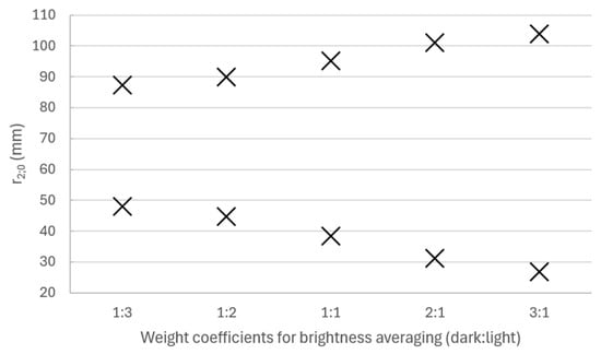
Figure 14.
Sensitivity of results to weight coefficient settings when using weighed average to detect the border between the well-mixed ring and settled particles.
The simple arithmetic average used in this study corresponds to the 1:1 case (where the gradient is cut halfway through). The results vary around this point significantly. This, however, is not a question of error or uncertainty, but rather of how the comparison method is designed. If the same approach is used for all analyzed cases, all errors are avoided. Using the simple average (i.e., equal weight coefficients) is the most natural approach. The weighted average analysis shown in Figure 14 can also be further used to evaluate the temporal behavior of the fluctuating interface.
4. Conclusions
- Lite LBM simulations of an axially mixed liquid–solid batch were carried out for several different particle drag force models, and the results were compared with the experimental findings. The tested models were the Brown and Lawler model [21], Equation (7), and Rong model [27], Equation (13), which are present in the software; as well as the Gidaspow model [28], Equation (14), which was implemented as a user-defined function.
- A simple and accessible comparison method for measuring near-off-bottom suspension flow patterns was newly adapted. The subjectivity of visual reads was eliminated by using computer image processing for both experimental data and simulation result renderings, allowing better comparability.
- It was found that the baffles deform the expected circular patterns when using impeller speeds below the just off-bottom suspension speed in a standard axially mixed baffled tank. The -norm was introduced as an effective tool to describe this phenomenon. It serves to quantify the effect of baffles on the symmetries in the system under different conditions, such as how the outer interface deforms more (p increases) when nearing the baffles at higher impeller speeds. This new two-parameter description can provide the required nuance for more thorough comparisons in the future.
- The simulation succeeded in replicating the flow patterns even without the formulation of the interphase forces considered important for the off-bottom suspension (though with non-negligible average errors of about 20% for the two dilute suspensions and 30% for the dense), underlining our point that the general behavior surrounding the off-bottom suspension comprises more than mechanics of the initial particle lift.
- The simulation results across configurations were generally closer to each other than to experimental data. We consider this a culmination of approximations—both methodical (imperfect calibration of visual conditions and general uncertainties surrounding the visual rendering of simulation results) and numerical (mainly the particle parceling and simplified contact model).
- Despite the simplifications, the Rong model [27], Equation (13), replicated the experiments better overall than the Brown and Lawler model [21], Equation (7), in percentages according to the assumption. The model of Rong [27], Equation (13), however, overestimated the outer interface radius at higher impeller speeds and higher solid fractions. The Gidaspow model [28], Equation (14), behaved well and remained in between the other two models, despite being originally devised for an Euler–Euler description. Its results were closer to the lone particle Brown and Lawler model [21], Equation (7), than to Rong [27], Equation (13). Of course, different regions of the tank may be better described using different models—in our case, it would be possible to conduct a differentiated comparison between the inner and outer shape, which we intend to explore in the future on a more established and rigorous basis. Following these points, the presented method can be a convenient aid for comparing the drag force and other models for different mixing cases.
Author Contributions
Conceptualization, F.R. and T.J.; methodology, F.R. and T.J.; software, F.R.; validation, F.R.; resources, T.J.; data curation, F.R. and T.J.; writing—original draft preparation, F.R.; writing—review and editing, F.R. and T.J.; visualization, F.R.; supervision, T.J.; project administration, T.J.; funding acquisition, F.R. and T.J. All authors have read and agreed to the published version of the manuscript.
Funding
This work was financially supported by the Student Grant Competition of Czech Technical University in Prague, SGS23/160/OHK2/3T/12.
Data Availability Statement
Since disclosing full raw visual data and all their follow-up processing would be cumbersome, data will be provided on request by the corresponding author in any required form.
Conflicts of Interest
The authors declare no conflicts of interest. The funders had no role in the design of the study; in the collection, analyses or interpretation of data; in the writing of the manuscript; or in the decision to publish the results.
Abbreviations
| Archimedes number | ||
| Smagorinsky coefficient | ||
| drag coefficient | ||
| drag coefficient of a lone steady particle | ||
| tank diameter | ||
| impeller diameter | ||
| particle diameter | ||
| particle drag force | ||
| modified Froude number | ||
| gravitational acceleration | ||
| impeller speed | ||
| just-suspended impeller speed (critical impeller speed) | ||
| p-norm exponent | ||
| interior interface radius of sedimented and mixed particles | ||
| exterior interface radius of sedimented and mixed particles | ||
| empirical proportionality constant for the Zwietering correlation | ||
| timestep | ||
| fluid velocity | ||
| fluid velocity | ||
| mass percentage of suspended solids to liquid in the Zwietering correlation | ||
| grid spacing | ||
| liquid fraction | ||
| solid/particle fraction | ||
| voidage function exponent | ||
| shear rate | ||
| mechanical power dissipation per unit mass of fluid phase | ||
| Kolmogoroff scale of dissipative eddies | ||
| dynamic viscosity | ||
| kinematic viscosity | ||
| liquid density | ||
| particle (solid) density |
References
- Derksen, J.J. Highly resolved simulations of solids suspension in a small mixing tank. AIChE J. 2012, 58, 3266–3278. [Google Scholar] [CrossRef]
- Ayranci, I.; Machado, M.B.; Madej, A.M.; Derksen, J.J.; Nobes, D.S.; Kresta, S.M. Effect of geometry on the mechanisms for off-bottom solids suspension in a stirred tank. Chem. Eng. Sci. 2012, 79, 163–176. [Google Scholar] [CrossRef]
- Derksen, J. Eulerian-Lagrangian simulations of settling and agitated dense solid-liquid suspensions—Achieving grid convergence. AIChE J. 2018, 64, 1147–1158. [Google Scholar] [CrossRef]
- Blais, B.; Lassaigne, M.; Goniva, C.; Fradette, L.; Bertrand, F. Development of an unresolved CFD–DEM model for the flow of viscous suspensions and its application to solid–liquid mixing. J. Comput. Phys. 2016, 318, 201–221. [Google Scholar] [CrossRef]
- Blais, B.; Bertrand, O.; Fradette, L.; Bertrand, F. CFD-dem simulations of early turbulent solid–liquid mixing: Prediction of suspension curve and just-suspended speed. Chem. Eng. Res. Des. 2017, 123, 388–406. [Google Scholar] [CrossRef]
- Tamburini, A.; Cipollina, A.; Micale, G.; Brucato, A.; Ciofalo, M. CFD simulations of dense solid–liquid suspensions in baffled stirred tanks: Prediction of suspension curves. Chem. Eng. J. 2011, 178, 324–341. [Google Scholar] [CrossRef]
- Tamburini, A.; Cipollina, A.; Micale, G.; Ciofalo, M.; Brucato, A. Dense solid–liquid off-bottom suspension dynamics: Simulation and experiment. Chem. Eng. Res. Des. 2009, 87, 587–597. [Google Scholar] [CrossRef]
- Hosseini, S.; Patel, D.; Ein-Mozaffari, F.; Mehrvar, M. Study of solid–liquid mixing in agitated tanks through electrical resistance tomography. Chem. Eng. Sci. 2010, 65, 1374–1384. [Google Scholar] [CrossRef]
- Barigou, M. Particle tracking in opaque mixing systems: An overview of the capabilities of PET and PEPT. Chem. Eng. Res. Des. 2004, 82, 1258–1267. [Google Scholar] [CrossRef]
- Raffel, M.; Willert, C.E.; Scarano, F.; Kähler, C.J.; Wereley, S.T.; Kompenhans, J. Particle Image Velocimetry: A Practical Guide; Springer: Cham, Switzerland, 2018. [Google Scholar]
- M-Star. Available online: https://mstarcfd.com/ (accessed on 31 March 2024).
- Chen, S.; Doolen, G.D. Lattice Boltzmann Method for Fluid Flows. Annu. Rev. Fluid Mech. 1998, 30, 329–364. [Google Scholar] [CrossRef]
- M-Star CFD Documentation. Available online: https://docs.mstarcfd.com/ (accessed on 31 March 2024).
- Sirasitthichoke, C.; Teoman, B.; Thomas, J.; Armenante, P.M. Computational prediction of the just-suspended speed, Njs, in stirred vessels using the lattice Boltzmann method (LBM) coupled with a novel mathematical approach. Chem. Eng. Sci. 2022, 251, 117411. [Google Scholar] [CrossRef]
- Giacomelli, J.J.; Van den Akker, H.E. Time Scales and turbulent spectra above the base of stirred vessels from large eddy simulations. Flow Turbul. Combust. 2020, 105, 31–62. [Google Scholar] [CrossRef]
- Giacomelli, J.J.; Van den Akker, H.E. A spectral approach of suspending solid particles in a turbulent stirred vessel. AIChE J. 2020, 67, e17097. [Google Scholar] [CrossRef]
- Kildashti, K.; Dong, K.; Yu, A. Contact force models for non-spherical particles with different surface properties: A Review. Powder Technol. 2023, 418, 118323. [Google Scholar] [CrossRef]
- Mao, Z.; Yang, C. Challenges in study of single particles and particle swarms. Chin. J. Chem. Eng. 2009, 17, 535–545. [Google Scholar] [CrossRef]
- Schiller, L.; Maumann, A. Über die grundlegenden Berechnungen bei der Schwerkraftaufbereitung. Z. Ver. Dtsch. Ing. 1933, 77, 318–320. [Google Scholar]
- DallaValle, J.M. Micromeritics, the Technology of Fine Particles; Pitman Pub. Corp: New York, NY, USA, 1948. [Google Scholar]
- Brown, P.P.; Lawler, D.F. Sphere drag and settling velocity revisited. J. Environ. Eng. 2003, 129, 222–231. [Google Scholar] [CrossRef]
- Brucato, A.; Grisafi, F.; Montante, G. Particle drag coefficients in turbulent fluids. Chem. Eng. Sci. 1998, 53, 3295–3314. [Google Scholar] [CrossRef]
- Khopkar, A.R.; Kasat, G.R.; Pandit, A.B.; Ranade, V.V. Computational fluid dynamics simulation of the solid suspension in a stirred slurry reactor. Ind. Eng. Chem. Res. 2006, 45, 4416–4428. [Google Scholar] [CrossRef]
- Pinelli, D.; Nocentini, M.; Magelli, F. Solids distribution in stirred slurry reactors: Influence of some mixer configurations and limits to the applicability of a simple model for predictions. Chem. Eng. Commun. 2001, 188, 91–107. [Google Scholar] [CrossRef]
- Fajner, D.; Pinelli, D.; Ghadge, R.S.; Montante, G.; Paglianti, A.; Magelli, F. Solids distribution and rising velocity of buoyant solid particles in a vessel stirred with multiple impellers. Chem. Eng. Sci. 2008, 63, 5876–5882. [Google Scholar] [CrossRef]
- Di Felice, R. The voidage function for fluid-particle interaction systems. Int. J. Multiphas. Flow 1994, 20, 153–159. [Google Scholar] [CrossRef]
- Rong, L.W.; Dong, K.J.; Yu, A.B. Lattice-boltzmann simulation of fluid flow through packed beds of uniform spheres: Effect of porosity. Chem. Eng. Sci. 2013, 99, 44–58. [Google Scholar] [CrossRef]
- Gidaspow, D. Multiphase Flow and Fluidization: Continuum and Kinetic Theory Descriptions; Elsevier Science: St. Louis, MO, USA, 2014. [Google Scholar]
- Ergun, S.; Orning, A.A. Fluid flow through randomly packed columns and Fluidized Beds. Ind. Eng. Chem. 1949, 41, 1179–1184. [Google Scholar] [CrossRef]
- Wen, C.Y.; Yu, Y.H. Mechanics of Fluidization. Chem. Eng. Prog. Symp. Ser. 1966, 162, 100–111. [Google Scholar]
- Wang, H.; Zhang, B.; Li, X.; Xiao, Y.; Yang, C. Modeling total drag force exerted on particles in dense swarm from experimental measurements using an inline image-based method. Chem. Eng. J. 2022, 431, 133485. [Google Scholar] [CrossRef]
- Ochieng, A.; Onyango, M.S. Drag models, solids concentration and velocity distribution in a stirred tank. Powder Technol. 2008, 181, 1–8. [Google Scholar] [CrossRef]
- ANSYS FLUENT 12.0 Theory Guide. Available online: https://www.afs.enea.it/project/neptunius/docs/fluent/html/th/main_pre.htm (accessed on 4 May 2024).
- Špidla, M.; Sinevič, V.; Jahoda, M.; Machoň, V. Solid particle distribution of moderately concentrated suspensions in a pilot plant stirred vessel. Chem. Eng. J. 2005, 113, 73–82. [Google Scholar] [CrossRef]
- Marchelli, F.; Hou, Q.; Bosio, B.; Arato, E.; Yu, A. Comparison of different drag models in CFD-dem simulations of spouted beds. Powder Technol. 2020, 360, 1253–1270. [Google Scholar] [CrossRef]
- Zwietering, T.N. Suspending of solid particles in liquid by agitators. Chem. Eng. Sci. 1958, 8, 244–253. [Google Scholar] [CrossRef]
- Rieger, F.; Ditl, P. Suspension of solid particles. Chem. Eng. Sci. 1994, 49, 2219–2227. [Google Scholar] [CrossRef]
- Jirout, T.; Rieger, F. Impeller design for mixing of suspensions. Chem. Eng. Res. Des. 2011, 89, 1144–1151. [Google Scholar] [CrossRef]
- Grenville, R.K.; Mak, A.T.C.; Brown, D.A.R. Suspension of solid particles in vessels agitated by axial flow impellers. Chem. Eng. Res. Des. 2015, 100, 282–291. [Google Scholar] [CrossRef]
- Jirout, T.; Jiroutová, D. Application of theoretical and experimental findings for optimization of mixing processes and equipment. Processes 2020, 8, 955. [Google Scholar] [CrossRef]
- Jirout, T.; Moravec, J.; Rieger, F.; Sinevič, V.; Špidla, M.; Sobolík, V.; Tihoň, J. Electrochemical Measurement of Impeller Speed For Off-Bottom Suspension. Chem. Process Eng. 2005, 26, 485–497. [Google Scholar]
- Micale, G.; Grisafi, F.; Brucato, A. Assessment of particle suspension conditions in stirred vessels by means of pressure gauge technique. Chem. Eng. Res. Des. 2002, 80, 893–902. [Google Scholar] [CrossRef]
- Teoman, B.; Sirasitthichoke, C.; Potanin, A.; Armenante, P.M. Determination of the just-suspended speed, Njs, in stirred tanks using electrical resistance tomography (ERT). AIChE J. 2021, 67, e17354. [Google Scholar] [CrossRef]
- Rettinger, C.; Rüde, U. A coupled lattice Boltzmann method and discrete element method for discrete particle simulations of particulate flows. Comput. Fluids 2018, 172, 706–719. [Google Scholar] [CrossRef]
- MATLAB Documentation. Available online: https://www.mathworks.com/help/matlab/index.html (accessed on 22 June 2024).
- Otsu, N. A threshold selection method from gray-level histograms. IEEE Trans. Syst. Man Cybern. 1979, 9, 62–66. [Google Scholar] [CrossRef]
- Poodiack, R.D.; Wood, W.E. Squigonometry: The Study of Imperfect Circles; Springer: Cham, Switzerland, 2022. [Google Scholar]
- Lagarias, J.C.; Reeds, J.A.; Wright, M.H.; Wright, P.E. Convergence properties of the Nelder–mead simplex method in low dimensions. SIAM J. Optim. 1998, 9, 112–147. [Google Scholar] [CrossRef]


Disclaimer/Publisher’s Note: The statements, opinions and data contained in all publications are solely those of the individual author(s) and contributor(s) and not of MDPI and/or the editor(s). MDPI and/or the editor(s) disclaim responsibility for any injury to people or property resulting from any ideas, methods, instructions or products referred to in the content. |
© 2025 by the authors. Licensee MDPI, Basel, Switzerland. This article is an open access article distributed under the terms and conditions of the Creative Commons Attribution (CC BY) license (https://creativecommons.org/licenses/by/4.0/).