TPG Conversion and Residual Oil Simulation in Heavy Oil Reservoirs

Abstract

The Threshold Pressure Gradient (TPG) phenomenon exerts a profound influence on fluid flow dynamics in heavy oil reservoirs. However, the discrepancies between the True Threshold Pressure Gradient (TTPG) and Pseudo-Threshold Pressure Gradient (PTPG) significantly impede accurate residual oil evaluation and rational field development planning. This study proposes a dual-exponential conversion model that effectively bridges the discrepancy between TTPG and PTPG, achieving an average deviation of 12.77–17.89% between calculated and measured TTPG values. Nonlinear seepage simulations demonstrate that TTPG induces distinct flow barrier effects, driving residual oil accumulation within low-permeability interlayers and the formation of well-defined “dead oil zones.” In contrast, the linear approximation inherent in PTPG overestimates flow initiation resistance, resulting in a 47% reduction in recovery efficiency and widespread residual oil enrichment. By developing a TTPG–PTPG conversion model and incorporating genuine nonlinear seepage characteristics into simulations, this study effectively mitigates the systematic errors arising from the linear PTPG assumption, thereby providing a scientific basis for accurately predicting residual oil distribution and enhancing oil recovery efficiency.

1. Introduction

Heavy oil reservoirs, characterized by high viscosity and complex seepage behavior, present critical challenges in oil and gas development [1,2]. During heavy oil seepage, a significant Threshold Pressure Gradient (TPG) phenomenon occurs due to fluid–rock interactions, where fluids require overcoming a critical driving force to initiate flow [3,4]. This TPG critically impacts reservoir sweep efficiency and recovery [5,6]. The True Threshold Pressure Gradient (TTPG) reflects the critical driving force for fluid transition from static to mobile states, influenced by factors such as crude oil viscosity, rock permeability, and temperature [7,8]. In contrast, the Pseudo-Threshold Pressure Gradient (PTPG) is an empirical value derived from linear extrapolation of the linear segment of flow curves, widely adopted to simplify non-Darcy flow models due to its straightforward experimental methodology [9,10].

However, substantial discrepancies exist between PTPG and TTPG, leading to ineffective guidance for field operations. Schlichting H. elucidated the formation mechanism of TTPG via boundary layer theory, demonstrating its inverse proportionality to pore diameter [7]. Yang Zhengming et al. established regression models for PTPG through core displacement experiments, yet deviations exceeding 30% were observed in low-permeability reservoirs compared with TTPG [11]. The nonlinear characteristics of TTPG result in “island-like” distributions of remaining oil in low-permeability zones, whereas linear extrapolation of PTPG oversimplifies these into continuous bands [12]. Simulations of the Chang 7 low-permeability reservoir in the Ordos Basin revealed that neglecting TTPG nonlinearity could induce prediction errors in the remaining oil saturation exceeding 25% [13]. Furthermore, TTPG exhibits exponential growth with decreasing permeability, causing residual oil retention between high- and low-permeability layers [14]. However, the linear assumption of PTPG weakens interlayer mobilization differences, overestimating waterflooding efficiency in high-permeability layers [15]. Existing studies confirm significant disparities between PTPG and TTPG; direct application of PTPG may lead to prediction discrepancies in the remaining oil distribution and overestimation of recovery by 15–20% [16].

TTPG is typically determined through micro-flow displacement pressure methods or dynamic flow experiments, requiring precise capture of fluid breakthrough pressure signals using high-precision pressure sensing systems [17,18]. However, such methods face practical limitations due to stringent equipment requirements [19]. PTPG, derived from linear extrapolation of flow curves, remains operationally convenient but fails to account for the nonlinear characteristics inherent in seepage curves [20].

This study enhances measurement accuracy by increasing pressure sensor resistance through circuit optimization, building upon conventional micro-flow displacement pressure methods. We establish a dual-exponential conversion model to link TTPG and PTPG using MATLAB R2016a regression analysis. The derived TTPG model is implemented in a nonlinear seepage simulator (NRSNL) to predict the residual oil distribution in heterogeneous reservoirs. This work fills a critical gap in heavy oil reservoir engineering by providing a scalable framework for indirect TTPG estimation and nonlinear seepage simulation. The findings offer practical implications for optimizing injection–production strategies, reducing residual oil accumulation, and improving recovery efficiency in complex reservoirs.

2. Experimental Materials and Methods

2.1. Experimental Materials

In the experiment, the oil samples were obtained from different oil field wellheads, specifically dehydrated heavy oils from wells 1# and 2#. The Heavy Oil Viscosity–Temperature Curve is shown in Figure 1 and Figure 2. The NB/SH/T 0509-2010 [21] “Test method for separation of asphalt into four fractions” standard was used to determine the relative content of the four components in the heavy oil samples from the oil fields. The parameters of the heavy oil samples are shown in

Table 1. Basic parameters of heavy oil samples.

Heavy Oil Sample Number	Saturate, %	Aromatic, %	Resin, %	Asphaltene, %	Viscosity at 30 °C, mPa·s
1#	47.35	31.13	16.23	5.30	612.10
2#	38.76	23.13	30.75	7.36	3912.65

below, and the core is artificial sandstone, with basic parameters as shown in

Table 2. Basic core parameters.

Core Number	Heavy Oil Sample	Length, cm	Diameter, cm	Porosity, %	Permeability, mD
1–7	1#	9.65	2.41	26.15	325.50
1–24	1#	9.49	2.49	31.52	1331.32
1–8	2#	9.04	2.50	24.80	328.07
1–25	2#	9.47	2.48	31.23	1336.83
1–49	2#	9.00	2.50	34.90	3021.33

.

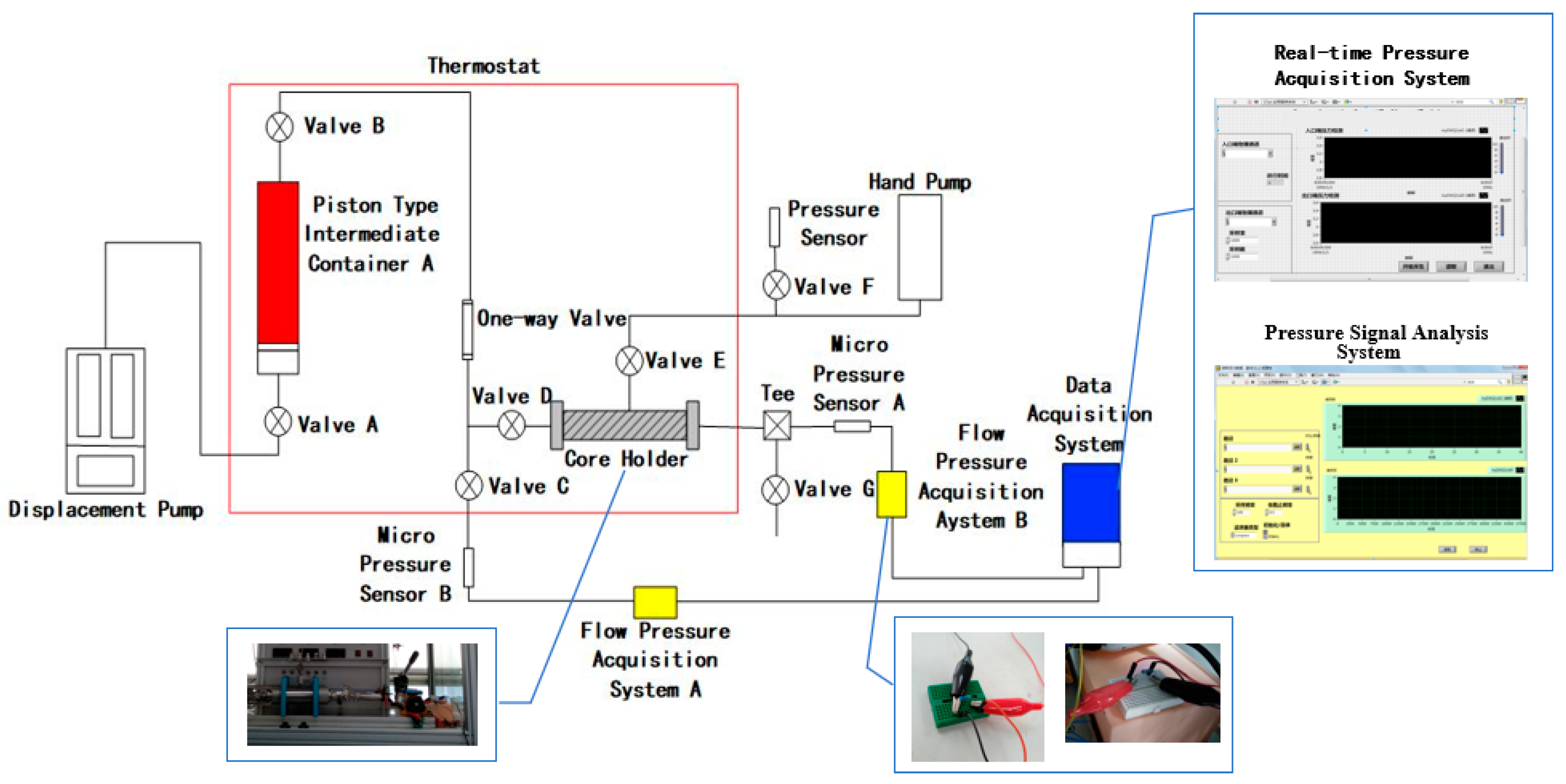
2.2. Experimental Methods

2.2.1. The Method for Measuring True Threshold Pressure Gradient (TTPG)

In core seepage experiments, the onset of fluid flow at the core outlet can be identified by an abrupt voltage signal change from the pressure differential sensor. Specifically, high-sensitivity pressure differential sensors are installed at both the inlet and outlet of the core. The sensitive elements of these sensors convert pressure differences into voltage signals. Initially, when the inlet pressure remains below TTPG, the pressure difference between the outlet and inlet approaches zero, resulting in a stable baseline voltage output from the sensor. As the inlet pressure gradually increases to TTPG, fluid invades the pore throats of the core, causing an instantaneous pressure surge at the outlet. This triggers a step-like voltage change in the differential sensor, with the moment of voltage jump corresponding to the initiation of fluid flow.

To achieve precise detection, this study utilizes a dual-channel pressure differential monitoring system by simultaneously deploying miniature pressure sensors at both ends of the core (Figure 3). When fluid begins flowing within the core, the outlet sensor converts the small pressure difference into a 4–20 mA current signal. This current is then passed through a shunt resistor (100 Ω), converting it into a voltage signal amplified by a factor of 1000. This amplification increases the voltage change corresponding to the initial pressure difference from 0.1 mV to 100 mV, effectively enhancing measurement accuracy by a factor of 1000. The enhanced signal is transmitted to a computer via a USB interface, where LabVIEW 2017 software performs millisecond-scale data filtering and pressure value inversion. Finally, the fluid flow initiation point is determined by analyzing the voltage abrupt change curve at the outlet.

This method utilizes high-precision hardware-based signal amplification and real-time software processing to overcome the limitations of conventional sensors, thereby ensuring accurate identification of TTPG and flow behavior during core flooding experiments.

The experimental procedures for determining TTPG are as follows:

1. Evacuate the core and saturate it with formation water;

2. Establish connate water saturation;

3. Age the core at a constant temperature for over 24 h;

4. Displace the core with a small flow rate using a pump.

As displacement progresses, the voltage signal at the core inlet gradually increases. When the inlet voltage reaches a specific critical threshold, the voltage signal from the outlet pressure collection system commences to rise. The moment of outlet voltage increase corresponds to the inlet voltage at that instant, which is then converted into a pressure value representing the TTPG.

2.2.2. The Method for Measuring Pseudo-Threshold Pressure Gradient (PTPG)

Experimental procedures for determining the Pseudo-Threshold Pressure Gradient are as follows [22,23]:

1. Evacuate the core and saturate it with formation water.

2. Establish connate water saturation.

3. Age the core at a constant temperature (e.g., 60 °C) for over 24 h.

4. Inject the oil sample into the core at displacement flow rates of 0.01, 0.03, 0.05, 0.1, and 0.2 mL/min. Maintain a stable inlet pressure and outlet flow rate for at least 30 min at each flow rate before proceeding to the next rate.

5. Plot the flow rate–pressure gradient curve, and extrapolate the linear segment to intersect the pressure gradient axis, where the x-intercept corresponds to PTPG.

2.2.3. Conversion Methods Between TTPG and TPTG

This study develops transformation models between TTPG and PTPG using MATLAB R2016a software. Two high-correlation models—a power–law function and an exponential function—are established to ensure precise conversion. To quantitatively assess the differences between pre- and post-conversion results, both TTPG and PTPG values are plotted on a Threshold Pressure Gradient (TPG) vs. fluid mobility diagram. This visualization reveals an exponential nonlinear relationship between TTPG and PTPG, demonstrating the critical requirement for model-derived conversion in accurate reservoir characterization.

3. Numerical Method

To investigate the influence of TTPG and PTPG on development performance in actual oil field operations, this study employed the NRSNL (Nonlinear Reservoir Simulation) software (Self-developed simulator) to analyze heavy oil reservoir characteristics and shear-thinning viscoplastic flow behavior in the offshore PL19-3 oil field. A mechanistic simulation model was developed to systematically evaluate TTPG/PTPG impacts on three critical development indices: residual oil distribution, recovery efficiency, and water-cut evolution. Methodological details of the numerical discretization and governing equations are documented in the works by Xin Xiankang (2017) [24] and Zhang Xu (2015) [25].

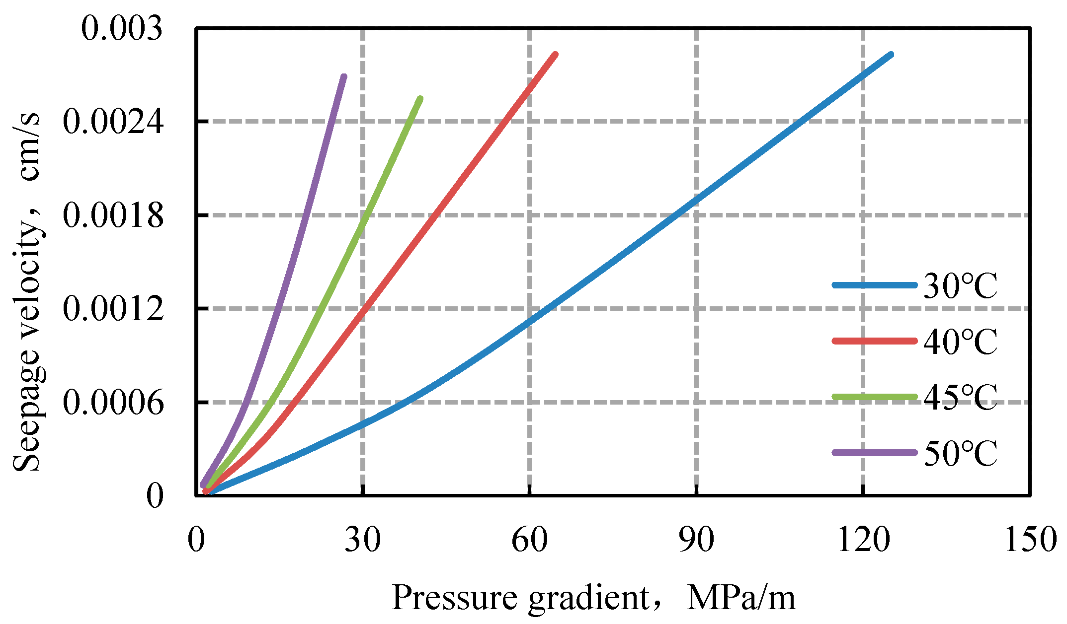
3.1. Nonlinear Seepage

The flow of heavy oil does not follow nonlinear seepage [25,26]. As shown in Figure 4.

Model (1): Nonlinear seepage accounting for TTPG (${\lambda }_0$) and PTPG ($\lambda$).

Model (2): Pseudolinear seepage incorporating the PTPG ($\lambda$).

$$v_{od}=\left\{\begin{array}{c}{\displaystyle \frac{k_{od}}{\frac{{\mu }_o}{\left[1-\frac{\lambda }{(\left|\frac{\partial {\Phi }_o}{\partial l_d}\right|-{\lambda }_0)+\lambda }\right]}}}{\displaystyle \frac{\partial {\Phi }_o}{\partial l_d}}\left|{\displaystyle \frac{\partial {\Phi }_o}{\partial l_d}}\right|>{\lambda }_0\\ 0\left|{\displaystyle \frac{\partial {\Phi }_o}{\partial l_d}}\right|\le {\lambda }_0\end{array}\right.and{v}_{wd}={\displaystyle \frac{k_{wd}}{{\mu }_w}}{\displaystyle \frac{\partial {\Phi }_w}{\partial l_d}}$$

(1)

$$v_{od}=\left\{\begin{array}{c}{\displaystyle \frac{k_{od}}{(\frac{{\mu }_o}{1-\frac{\lambda }{\left|\frac{\partial {\Phi }_o}{\partial l_d}\right|}})}}{\displaystyle \frac{\partial {\Phi }_o}{\partial l_d}}\left|{\displaystyle \frac{\partial {\Phi }_o}{\partial l_d}}\right|>\lambda \\ 0\left|{\displaystyle \frac{\partial {\Phi }_o}{\partial l_d}}\right|\le \lambda \end{array}\right.and{v}_{wd}={\displaystyle \frac{k_{wd}}{{\mu }_w}}{\displaystyle \frac{\partial {\Phi }_w}{\partial l_d}}$$

(2)

where ${\mathrm{v}}_{\mathrm{o}\mathrm{d}}$ are the oil velocities in the ${\mathrm{l}}_1$ = x, ${\mathrm{l}}_2$ = y, and ${\mathrm{l}}_3=\mathrm{z}$ directions in m/s; ${\mathrm{k}}_{\mathrm{o}\mathrm{d}}\mathrm{ }$ are the oil permeabilities in the x, y, and z directions in ${\mathrm{m}}^2$; ${\mathrm{\mu }}_{\mathrm{o}}$ and ${\mathrm{\mu }}_{\mathrm{w}}$ are the viscosities of oil and water in Pa·s; $\partial$ is a symbol used to denote partial derivatives; ${\mathrm{\Phi }}_{\mathrm{o}}={\mathrm{p}}_{\mathrm{o}}-{\mathrm{\rho }}_{\mathrm{o}}\mathrm{g}\mathrm{D}$ and ${\mathrm{\Phi }}_{\mathrm{w}}={\mathrm{p}}_{\mathrm{w}}-{\mathrm{\rho }}_{\mathrm{w}}\mathrm{g}\mathrm{D}$ in Pa; ${\mathrm{p}}_{\mathrm{o}}$ and ${\mathrm{p}}_{\mathrm{w}}$ are the pressures of the oil and water phases in Pa; ${\mathrm{\rho }}_{\mathrm{o}}$ and ${\mathrm{\rho }}_{\mathrm{w}}$ are the oil and water densities in ${\mathrm{kg}/\mathrm{m}}^3$; g is the gravitational acceleration in ${\mathrm{m}/\mathrm{s}}^2$; D is the vertical height in m; ${\mathrm{v}}_{\mathrm{w}\mathrm{d}}\mathrm{ }$ are the water velocities in the x, y, and z directions in m/s; and ${\mathrm{k}}_{\mathrm{w}\mathrm{d}}\mathrm{ }$ are the water permeabilities in the x, y, and z directions in ${\mathrm{m}}^2$.

3.2. Flow Model

For the oil component, this is calculated as follows:

$${\displaystyle \frac{\partial }{\partial x}}\left[{\rho }_{os}{\displaystyle \frac{k_a{k}_{ro}}{B_o{\mu }_{co1}}}\left({\displaystyle \frac{\partial p_o}{\partial x}}-{\rho }_{o}g{\displaystyle \frac{\partial D}{\partial x}}\right)\right]+{\displaystyle \frac{\partial }{\partial y}}\left[{\rho }_{os}{\displaystyle \frac{k_a{k}_{ro}}{B_o{\mu }_{co2}}}\left({\displaystyle \frac{\partial p_o}{\partial y}}-{\rho }_{o}g{\displaystyle \frac{\partial D}{\partial y}}\right)\right]+{\displaystyle \frac{\partial }{\partial z}}\left[{\rho }_{os}{\displaystyle \frac{k_a{k}_{ro}}{B_o{\mu }_{co3}}}\left({\displaystyle \frac{\partial p_o}{\partial z}}-{\rho }_{o}g{\displaystyle \frac{\partial D}{\partial z}}\right)\right]+q_o={\displaystyle \frac{\partial }{\partial t}}\left({\rho }_{os}{\displaystyle \frac{\varphi S_o}{B_o}}\right)$$

(3)

For the water component, this is calculated as follows:

$${\displaystyle \frac{\partial }{\partial x}}\left[{\rho }_{ws}{\displaystyle \frac{k_a{k}_{rw}}{B_w{\mu }_w}}\left({\displaystyle \frac{\partial p_w}{\partial x}}-{\rho }_{w}g{\displaystyle \frac{\partial D}{\partial x}}\right)\right]+{\displaystyle \frac{\partial }{\partial y}}\left[{\rho }_{ws}{\displaystyle \frac{k_a{k}_{rw}}{B_w{\mu }_w}}\left({\displaystyle \frac{\partial p_w}{\partial y}}-{\rho }_{w}g{\displaystyle \frac{\partial D}{\partial y}}\right)\right]+{\displaystyle \frac{\partial }{\partial z}}\left[{\rho }_{ws}{\displaystyle \frac{k_a{k}_{rw}}{B_w{\mu }_w}}\left({\displaystyle \frac{\partial p_w}{\partial z}}-{\rho }_{ws}g{\displaystyle \frac{\partial D}{\partial z}}\right)\right]+q_w={\displaystyle \frac{\partial }{\partial t}}\left({\rho }_{ws}{\displaystyle \frac{\varphi S_w}{B_w}}\right)$$

(4)

In the two equations above, $\rho$_os and $\rho$_ws are the densities of oil and water in the ground standard conditions in kg/m³; ka is the absolute permeability of porous media in m²; kro and krw are the relative permeabilities of oil and water in fraction; q_o and q_w are the mass flow rates of oil and water in the ground standard conditions in kg/s; Bo and Bw are the oil and water formation volume factors in m³/m³; and S_o and S_w are the oil saturation and water saturation in fraction.

In addition to the two continuity differential equations, there are the following auxiliary equations and state equations. The auxiliary equations included the following:

$$S_o+S_w=1$$

(5)

3.3. IMPES

The difference equation of Equation (3) was given as follows:

$$\begin{gathered} {\displaystyle \frac{m_{oxi+\frac{1}{2},j,k}\frac{{\Phi }_{oi+1,j,k}^{n+1}-{\Phi }_{oi,j,k}^{n+1}}{0.5\left(\Delta x_{i+1}+\Delta x_i\right)}-m_{oxi-\frac{1}{2},j,k}\frac{{\Phi }_{oi,j,k}^{n+1}-{\Phi }_{oi-1,j,k}^{n+1}}{0.5\left(\Delta x_i+\Delta x_{i-1}\right)}}{\Delta x_i}} \\ +{\displaystyle \frac{m_{oyi,j+\frac{1}{2},k}\frac{{\Phi }_{oi,j+1,k}^{n+1}-{\Phi }_{oi,j,k}^{n+1}}{0.5\left(\Delta y_{i+1}+\Delta y_i\right)}-m_{oyi,j-\frac{1}{2},k}\frac{{\Phi }_{oi,j,k}^{n+1}-{\Phi }_{oi,j-1,k}^{n+1}}{0.5\left(\Delta y_i+\Delta y_{i-1}\right)}}{\Delta y_i}} \\ +{\displaystyle \frac{m_{ozi,j,k+\frac{1}{2}}\frac{{\Phi }_{oi,j,k+1}^{n+1}-{\Phi }_{oi,j,k}^{n+1}}{0.5\left(\Delta z_{i+1}+\Delta z_i\right)}-m_{ozi,j,k-\frac{1}{2}}\frac{{\Phi }_{oi,j,k}^{n+1}-{\Phi }_{oi,j,k-1}^{n+1}}{0.5\left(\Delta z_i+\Delta z_{i-1}\right)}}{\Delta z_i}} \\ +q_{oi,j,k}={\displaystyle \frac{1}{\Delta t}}\left[{\left({\displaystyle \frac{\varphi {\rho }_o{S}_o}{B_o}}\right)}_{i,j,k}^{n+1}-{\left({\displaystyle \frac{\varphi {\rho }_o{S}_o}{B_o}}\right)}_{i,j,k}^n\right] \end{gathered}$$

(6)

where the subscripts i, j, and k are the coordinate markers in the grid; the superscript n is the time marker; $\Delta$x, $\Delta$y, and $\Delta$z are the step length (m) in the direction of x, y, and z; and ${\mathrm{m}}_{\mathrm{o}\mathrm{x}}={\displaystyle \frac{{\mathrm{k}}_{\mathrm{a}}{\mathrm{k}}_{\mathrm{r}\mathrm{o}}}{{\mathrm{B}}_{\mathrm{o}}{\mathrm{\mu }}_{\mathrm{c}\mathrm{o}1}}},{\mathrm{m}}_{\mathrm{o}\mathrm{y}}={\displaystyle \frac{{\mathrm{k}}_{\mathrm{a}}{\mathrm{k}}_{\mathrm{r}\mathrm{o}}}{{\mathrm{B}}_{\mathrm{o}}{\mathrm{\mu }}_{\mathrm{c}\mathrm{o}2}}},\mathrm{a}\mathrm{n}\mathrm{d}{\mathrm{m}}_{\mathrm{o}\mathrm{z}}={\displaystyle \frac{{\mathrm{k}}_{\mathrm{a}}{\mathrm{k}}_{\mathrm{r}\mathrm{o}}}{{\mathrm{B}}_{\mathrm{o}}{\mathrm{\mu }}_{\mathrm{c}\mathrm{o}3}}}$ in m²/Pa·s.

In this work, these equations were solved by the IMPES with the auxiliary capillary and saturation equations under the boundary and initial conditions. More details can be found in [24,25].

3.4. The Nonlinear Seepage Simulator (NRSNL)

The NRSNL (Nonlinear Reservoir Simulation) model establishes the Threshold Pressure Gradient (TPG) by analyzing flow rate variations observed in the same reservoir across different temporal or spatial scales during field development operations [25]. This model introduces the concept of variable TPG, specifically distinguishing between TTPG and PTPG, which are implemented into the fluid flow framework via the MINPTH keyword (for TTPG) and PSDPTH keyword (for PTPG) within the numerical simulation system.

3.5. Establishment of Mechanistic Model

Considering the characteristics of the offshore PL19-3 reservoir and its fluid properties, a mechanistic model is established to investigate the effects of TTPG and PTPG on the residual oil distribution, recovery factor, and water cut. The base model consists of an inverted nine-spot well pattern (with central water injection). The model is configured with three layers, each having a thickness of 10 m. The permeabilities of the layers are 300 mD, 600 mD, and 900 mD, respectively; the permeability contrast is 3. The crude oil viscosity is 200 mPa·s. The well spacing is set to 450 m. The schematic of the base model is presented in Figure 5.

Using the oil–water two-phase seepage module of the NRSNL nonlinear seepage software (Self-developed simulator), a mechanistic model of size 1000 × 1000 × 3 is established to compare the differences in residual oil distribution, recovery factor, and water cut caused by TTPG and PTPG. The basic parameters of the model are shown in

Table 3. Numerical simulation plan.

Numerical Simulation Plan	Application Model	Number of Layers	Permeability, mD	TTPG, MPa·m−1	PTPG, MPa·m−1
A	Model (1), Equation (1)	1	300	0.0058	0.2121
		2	600	0.0037	0.0963
		3	900	0.0029	0.0546
B	Model (2), Equation (2)	1	300	/	0.2121
		2	600	/	0.0963
		3	900	/	0.0546

.

4. Results and Discussion

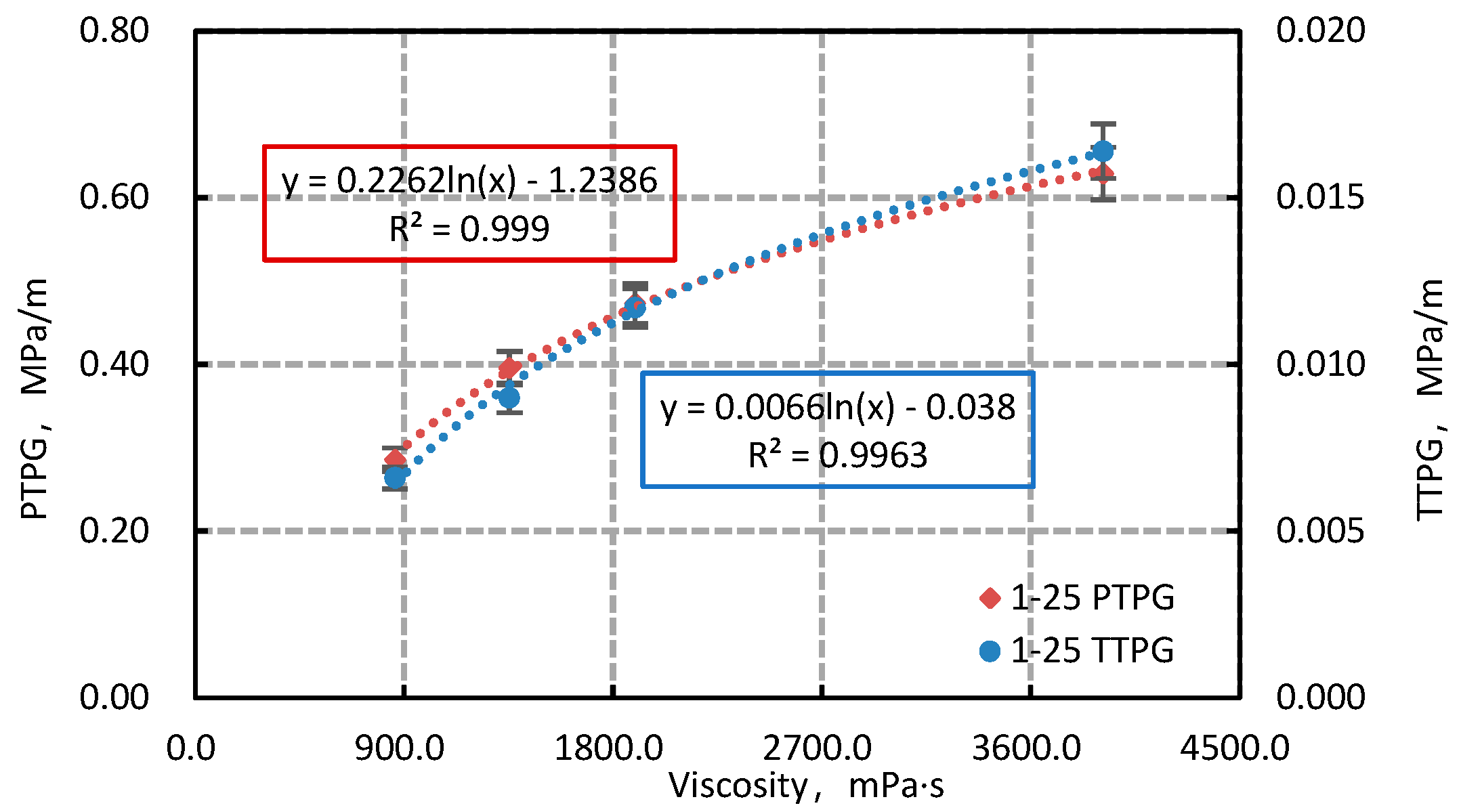
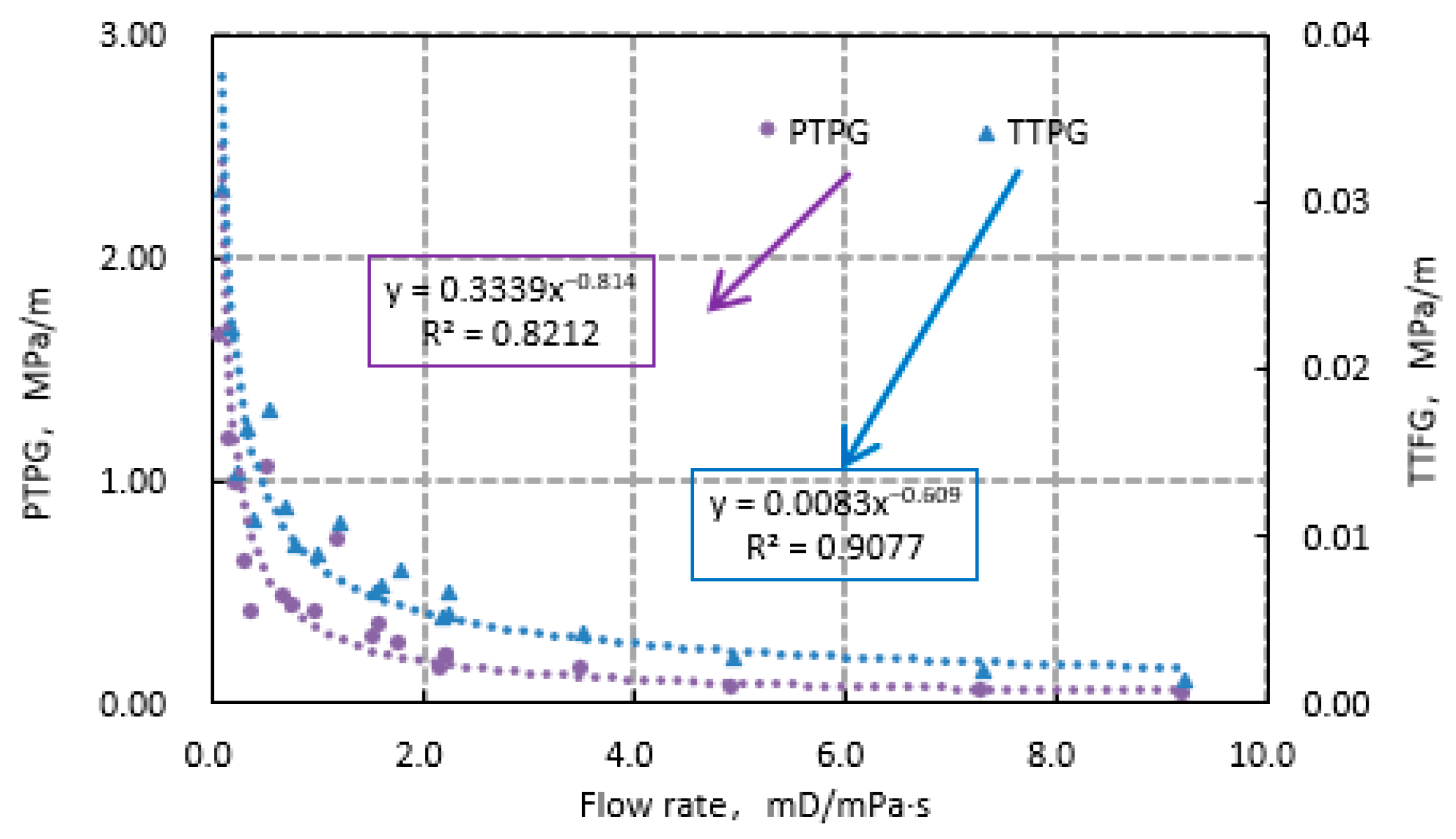
4.1. Conversion Relationship Between TTPG and PTPG

TTPG is determined using the methodology outlined in Section 2.2.1, while the PTPG is derived via the approach described in Section 2.2.2. The experimental seepage curve results are presented in Figure 6, Figure 7, Figure 8, Figure 9 and Figure 10.

PTPG is defined as the intersection value obtained by linearly extrapolating the linear segment of the seepage curve to the pressure gradient axis (abscissa). All seepage curve fitting equations in Table 4 are univariate linear regression equations:

y = kx + b

(7)

y: Flow velocity (cm/s)

x: Pressure gradient (MPa/m)

k: Slope (reflecting fluid mobility)

b: Intercept (directly related to PTPG). Corresponding regression equations for seepage behavior, PTPG values, and TTPG values are summarized in Table 4.

Table 4. Seepage equation and TTPG/PTGP results of heavy oil.

Core Numbering	Heavy Oil Sample	Temperature, °C	Seepage Curve Fitting Equation	Correlation Coefficient	PTPG, MPa·m−1	TTPG, MPa·m−1
1–8	2#	30	y = 0.0000170x − 0.0000280	0.9974	1.6471	0.0307
		40	y = 0.0000344x − 0.0000403	0.9928	1.1715	0.0225
		45	y = 0.0000498x − 0.0000488	0.9969	0.9799	0.0137
		50	y = 0.0000710x − 0.0000286	0.9917	0.4028	0.0110
1–25	2#	30	y = 0.0001103x − 0.0000694	0.9998	0.6292	0.0164
		40	y = 0.0002851x − 0.0001349	0.9992	0.4732	0.0117
		45	y = 0.0003876x − 0.0001534	0.9999	0.3958	0.0090
		50	y = 0.0005315x − 0.0001518	0.9999	0.2856	0.0066
1–49	2#	30	y = 0.0002901x − 0.0001241	0.9998	0.4278	0.0095
		40	y = 0.0005861x − 0.0001666	0.9999	0.3413	0.0070
		45	y = 0.0006855x − 0.0001408	0.9992	0.2054	0.0052
		50	y = 0.0008938x − 0.0001357	0.9997	0.1518	0.0042
1–7	1#	30	y = 0.0001786x − 0.0001866	0.9994	1.0441	0.0177
		40	y = 0.0003132x − 0.0002267	0.9994	0.7238	0.0108
		45	y = 0.0004536x − 0.0001151	0.9985	0.2537	0.0079
		50	y = 0.0006263x − 0.0001257	0.9998	0.2007	0.0067
1–24	1#	30	y = 0.0009229x − 0.0001312	0.9986	0.1422	0.0052
		40	y = 0.0015222x − 0.0000880	0.9991	0.0578	0.0027
		45	y = 0.0018016x − 0.0000759	0.9995	0.0421	0.0019
		50	y = 0.0021171x − 0.0000683	1.0000	0.0323	0.0014

Table 4. Seepage equation and TTPG/PTGP results of heavy oil.

Core Numbering	Heavy Oil Sample	Temperature, °C	Seepage Curve Fitting Equation	Correlation Coefficient	PTPG, MPa·m−1	TTPG, MPa·m−1
1–8	2#	30	y = 0.0000170x − 0.0000280	0.9974	1.6471	0.0307
		40	y = 0.0000344x − 0.0000403	0.9928	1.1715	0.0225
		45	y = 0.0000498x − 0.0000488	0.9969	0.9799	0.0137
		50	y = 0.0000710x − 0.0000286	0.9917	0.4028	0.0110
1–25	2#	30	y = 0.0001103x − 0.0000694	0.9998	0.6292	0.0164
		40	y = 0.0002851x − 0.0001349	0.9992	0.4732	0.0117
		45	y = 0.0003876x − 0.0001534	0.9999	0.3958	0.0090
		50	y = 0.0005315x − 0.0001518	0.9999	0.2856	0.0066
1–49	2#	30	y = 0.0002901x − 0.0001241	0.9998	0.4278	0.0095
		40	y = 0.0005861x − 0.0001666	0.9999	0.3413	0.0070
		45	y = 0.0006855x − 0.0001408	0.9992	0.2054	0.0052
		50	y = 0.0008938x − 0.0001357	0.9997	0.1518	0.0042
1–7	1#	30	y = 0.0001786x − 0.0001866	0.9994	1.0441	0.0177
		40	y = 0.0003132x − 0.0002267	0.9994	0.7238	0.0108
		45	y = 0.0004536x − 0.0001151	0.9985	0.2537	0.0079
		50	y = 0.0006263x − 0.0001257	0.9998	0.2007	0.0067
1–24	1#	30	y = 0.0009229x − 0.0001312	0.9986	0.1422	0.0052
		40	y = 0.0015222x − 0.0000880	0.9991	0.0578	0.0027
		45	y = 0.0018016x − 0.0000759	0.9995	0.0421	0.0019
		50	y = 0.0021171x − 0.0000683	1.0000	0.0323	0.0014

As illustrated in Figure 11, Figure 12, Figure 13, Figure 14 and Figure 15, the influence of heavy oil viscosity on the TTPG and PTPG exhibits identical trends. Specifically, both TTPG and PTPG demonstrate logarithmic increases with rising viscosity. Notably, excluding cores 1–25, all experimental results indicate that PTPG exhibits a greater rate of increase compared to TTPG as viscosity rises. PTPG exhibits significantly higher sensitivity to viscosity than TTPG (with an average sensitivity coefficient 1.8 times higher). In high-viscosity heavy oil (sample 2#), the measurement deviation of PTPG can reach up to 200% of that of TTPG (Figure 11). Consequently, when applying PTPG to predict reservoir productivity or optimize well patterns in field operations, higher viscosity heavy oils will inherently introduce larger deviations due to the amplified sensitivity of PTPG to viscosity variations [27].

The relationship curve between the PTPG and TTPG with flow rate is shown in Figure 16. The PTPG is much larger than TTPG, with some PTPG even exceeding TTPG by two orders of magnitude. It is not suitable to use the PTPG to calculate well patterns, well spacing, production capacity, etc., in practical development applications.

This study establishes a relationship between TTPG obtained from detecting flow pressure signals and PTPG. This allows the calculation of TTPG based on PTPG, which effectively resolves the difficulty in measuring TTPG. Multiple formulas were fitted using MATLAB R2016a software, and two formulas with high correlation coefficients were selected. Formula one represents a power function relationship, while formula two represents a double exponential function relationship. In these formulas, ${\lambda }_0$ represents TTPG, and $\lambda$ represents PTPG.

Relational formula one:

$${\lambda }_0=0.01696\ast {\lambda }^{0.9211}+0.001735$$

(8)

Among them, the multiple correlation coefficient is 0.9254.

Relational formula two:

$${\lambda }_0=0.007734\ast e^{0.8324\ast \lambda }-0.00718\ast e^{-4.099\ast \lambda }$$

(9)

Among them, the multiple correlation coefficient is 0.9410.

The experimental values of TTPG calculated from the two formulas and their relationship with flow rate are shown in the curve in Figure 17 below.

From the results shown in Figure 17, it can be observed that after converting PTPG to TTPG, there is a good agreement with the experimental results. After conversion using Formula (8), the average deviation between the obtained TTPG and the measured Threshold Pressure Gradient is 17.89%. After conversion using Formula (9), the average deviation is 12.77%. The relationship between TTPG and the flow rate after conversion closely matches the relationship between the measured values and the flow rate curve. The coefficients and exponent values of the curve fitting formulas are very close, indicating the reliability of the conversion formulas. Furthermore, the results obtained from Formula (9) are closer to the experimentally measured TTPG. The aforementioned conversion formulas between TTPG and PTPG can help oil fields indirectly obtain TTPGs of cores through seepage curves. This method is simple and conducive to practical applications in oil fields.

4.2. Numerical Simulation of Residual Oil in Heavy Oil Reservoirs

The rheological curve for the heavy oil in the PL19-3 field is depicted in Figure 16, while the seepage curve is illustrated in Figure 18.

The distribution of residual oil after 20 years of production in each layer is shown in Figure 19 and Figure 20. The final water cut and other results are presented in Figure 21 and Figure 22, respectively.

Through comparative simulations of the nonlinear seepage model (Model 1) and pseudolinear model (Model 2) from Figure 4, significant disparities in residual oil distribution and development index predictions were identified. In the nonlinear model, the coupling effect of TTPG and PTPG resulted in residual oil predominantly accumulating in low-permeability interlayers between injector–producer well pairs, forming immobile oil zones [28,29]. Concurrently, distinct preferential flow channels developed between injection and production wells [22]. This distribution pattern aligns with the dynamic TTPG characteristics observed in core flow curves—when pressure gradients exceed TTPG thresholds, permeability abruptly decreases in low-permeability zones, creating flow barriers, while high-permeability zones maintain low-resistance flow [30,31].

In contrast, the pseudolinear model excessively suppresses flow initiation pressure. This led to ineffective breakthrough of injected water into low-permeability layers, resulting in dispersed residual oil distribution across all layers and failure to establish effective displacement systems between wells [32]. Consequently, the recovery factor dropped to 5.89%, a 47% decrease compared to the nonlinear model. Further analysis (Figure 22 and Figure 23) revealed that excessive PTPG increased flow resistance by 2.3-fold, causing premature water breakthrough in producer wells (water cut reaching 97.98%). The nonlinear model, however, dynamically adjusted permeability via TTPG, achieving a smoother water cut increase (95.66%) and elevated recovery factor (11.14%). These discrepancies validate the indispensability of TTPG in characterizing heterogeneous reservoir seepage behaviors and expose the systematic errors introduced by PTPG’s linear simplification.

Practically, we recommend indirect TTPG estimation via the established TTPG–PTPG conversion model (Equations (8) and (9)) and adoption of nonlinear seepage simulators (NRSNL) to optimize development plans. This approach enhances prediction accuracy for residual oil distribution and improves recovery efficiency in heavy oil reservoirs.

Therefore, the linear assumption of PTPG inherently overestimates—erroneously—the critical pressure required to initiate fluid flow (i.e., overestimates flow initiation resistance), particularly for high-viscosity heavy oil in low-permeability layers. This directly results in the underestimation of the displacement capability of injected water in low-permeability layers within both numerical simulation predictions and practical development scheme designs. Consequently, injected water is forced to prematurely and intensively break through high-permeability layers, forming ineffective water flow channels (premature water channeling). This undermines the possibility of establishing an effective pressure-driven system and uniform displacement front between injection wells and production wells (disrupting the injection–production system), ultimately leading to the ineffective trapping of crude oil in various locations within the reservoir. By developing a TTPG–PTPG conversion model (Equations (8) and (9)) and incorporating genuine nonlinear seepage characteristics into simulations (accounting for TTPG), this study effectively mitigates the systematic errors arising from the linear PTPG assumption, thereby providing a scientific basis for accurately predicting residual oil distribution and enhancing oil recovery efficiency.

5. Conclusions

(1) This study achieved precise True Threshold Pressure Gradient (TTPG) measurement using high-sensitivity differential pressure sensors and signal amplification technology, overcoming limitations of traditional micro-flow methods dependent on high equipment precision. A dual-exponential conversion model for PTPG and TTPG was developed, validated by MATLAB fitting with an average deviation of 12.77%–17.89%, providing a feasible solution for rapid TTPG estimation in field applications.

(2) Numerical simulations based on the TTPG model effectively captured non-Darcy flow features, revealing injected water advancing along high-permeability layers and forming “dead oil zones” in low-permeability areas. In contrast, the linear PTPG assumption overestimated initiation resistance, leading to residual oil retention across all layers and a recovery factor prediction error of up to 47%, highlighting TTPG’s indispensability in heavy oil reservoir development.

(3) Using the PL19-3 oilfield (Ordos Basin) as a case study, nonlinear seepage simulations considering TTPG demonstrated that residual oil was primarily concentrated in dead oil zones between injector–producer well pairs, with distinct water drive channels and significantly higher recovery factors compared to quasilinear simulations (considering only PTPG). The PTPG quasilinear assumption, however, overestimated threshold pressure and caused excessive flow resistance, disconnected injection–production systems, increased residual oil volume, early water coning, and elevated water cut, resulting in a much lower recovery factor.

(4) These findings underscore the importance of accurately selecting TTPG parameters in numerical simulations to reliably predict development performance and optimize injection–production schemes for heavy oil reservoirs.

References

1. Dong, C.; Gong, S.; Lai, J.; Huang, S.; Li, B.; Li, Y. Experimental analysis and research on physical properties of heavy oil in offshore oilfields. Petrochem. Technol. 2009, 26, 161–162. [Google Scholar] [CrossRef]
2. Spiecker, P.M.; Gawrys, K.L.; Trail, C.B.; Kilpatrick, P.K. Effects of petroleum resins on asphaltene aggregation and water-in-oil emulsion formation. Colloids Surf. A Physicochem. Eng. Asp. 2003, 220, 9–27. [Google Scholar] [CrossRef]
3. Zhao, K. Study on Cold—Production Technology for Heavy-Oil Reservoirs with Strong Edge and Bottom Water in Zhan29 Block of Taiping Oilfield. Petrochem. Technol. 2019, 26, 83–84. [Google Scholar] [CrossRef]
4. Fingas, M.; Fieldhouse, B. Studies on crude oil and petroleum product emulsions: Water resolution and rheology. Colloids Surf. A Physicochem. Eng. Asp. 2009, 333, 67–81. [Google Scholar] [CrossRef]
5. Balhoff, M.T.; Thompson, K.E. Modeling the steady flow of yield stress fluids in packed beds. AIChE J. 2004, 50, 3034–3048. [Google Scholar] [CrossRef]
6. De Castro, A.R.; Radilla, G. Flow of yield stress and C arreau fluids through rough-walled rock fractures: Prediction and experiments. Water Resour. Res. 2017, 53, 6197–6217. [Google Scholar] [CrossRef]
7. Schlichting, H. Boundary Layer Theory; Science Press: Beijing, China, 1988. [Google Scholar]
8. Ke, W.L.; Wang, W.Y.; You, Y.; Ouyang, Y.L.; Yang, L.J.; Li, Q.H. Research on determination method of start-up pressure gradient for nonlinear seepage. Petrochem. Ind. Appl. 2013, 32, 1–4. [Google Scholar] [CrossRef]
9. Zhang, W.; Dai, J.W.; Wang, Y.H.; Tu, Y. Experimental study on enhanced oil recovery of offshore heavy oil reservoirs in high-ultra-high water cut stage. Bull. Geol. Sci. Technol. 2022, 41, 193–199. [Google Scholar] [CrossRef]
10. Wang, W.Y.; Yu, G.M.; Ke, W.L.; Wang, Y.; Ge, Y. Experimental study of nonlinear seepage for heavy oil. Pet. Exp. Geol. 2013, 4, 4. [Google Scholar] [CrossRef]
11. Yang, Z.M. Porous Flow Mechanics for Low Permeability Reservoirs and Its Application. Grad. Sch. Chin. Acad. Sci. 2007, 22, 96–99. [Google Scholar] [CrossRef]
12. Guo, R.; Li, P.F. Research on Petrosite heavy oil module algorithm. China New Technol. Prod. 2013, 21, 1. [Google Scholar] [CrossRef]
13. Ren, L. The Numerical Simulation Applied Technological Research of Chang 7 Super-Low Permeability Reservoir Water Injection Development. Master’s Thesis, Xi’an Petroleum University, Xi’an, China, 2012. [Google Scholar] [CrossRef]
14. Zhang, Y.; Wu, X.; Guo, Q.; Zhang, Z.; Cai, M. Nonlinear Seepage Behaviors of Pore-Fracture Sandstone under Hydro-Mechanical Coupling. Crystals 2022, 12, 373. [Google Scholar] [CrossRef]
15. Yang, Z.M.; Yu, R.Z.; Su, Z.X. Numerical simulation of the nonlinear flow in ultra-low permeability reservoirs. Pet. Explor. Dev. 2010, 37, 94–98. [Google Scholar] [CrossRef]
16. Cheng, K.Y.; Qi, Z.L.; Tian, J.; Yan, W.D.; Huang, X.L.; Huang, S.W. Change law of reservoir property during multi-cycle steam stimulation in heavy oil reservoir: A case study of HJ Oilfield. Reserv. Eval. Dev. 2022, 5, 12. [Google Scholar] [CrossRef]
17. Ke, W.L. Research on Nonlinear Percolation Law of Heavy Oil. Diploma Thesis, Yangtze University, Jingzhou, China, 2013. [Google Scholar]
18. Orgéas, L.; Idris, Z.; Geindreau, C.; Bloch, J.-F.; Auriault, J.-L. Modelling the flow of power-law fluids anisotropic porous media at low-pore reynolds number. Chem. Eng. Sci. 2006, 61, 4490–4502. [Google Scholar] [CrossRef]
19. Dong, S.; Liu, Z.; Yang, H.; Zhu, M.; Li, Z.; Sun, Z. A nonlinear seepage theory model is developed using nuclear magnetic experiment and fractal theory. Phys. Fluids 2024, 36, 17. [Google Scholar] [CrossRef]
20. Tao, G.; Huang, Z.; Xiao, H.L.; Zhao, W.; Luo, Q.S. A new nonlinear seepage model for clay soil considering the initial hydraulic gradient of microscopic seepage channels. Comput. Geotech. 2023, 154, 105179. [Google Scholar] [CrossRef]
21. NB/SH/T 0509; Test Method for Separation of Asphalt into Four Fractions. National Energy Administration: Beijing, China, 2010.
22. Ning, L.H. Experimental method and application of pressure gradient determination of heavy oil to be started. J. Coll. Univ. Petrochem. Ind. 2011, 24, 59–63. [Google Scholar] [CrossRef]
23. Tian, J.; Xu, J.F.; Cheng, L.S. Characterization and physical simulation method of starting pressure gradient for common heavy oil. J. Southwest Univ. Pet. Nat. Sci. Ed. 2009, 31, 158–162. [Google Scholar] [CrossRef]
24. Xin, X.K.; Li, Y.; Yu, G.; Wang, W.; Zhang, Z.; Zhang, M.; Ke, W.; Kong, D.; Wu, K.; Chen, Z. Non-Newtonian Flow Characteristics of Heavy Oil in the Bohai Bay Oilfield: Experimental and Simulation Studies. Energies 2017, 10, 1698. [Google Scholar] [CrossRef]
25. Zhang, X. Study and Application of Numerical Simulation of Nonlinear Percolation of Heavy Oil in Water Drive. Master’s Thesis, Yangtze University, Jingzhou, China, 2015. [Google Scholar]
26. You, X.; Li, S.; Kang, L.; Cheng, L. A Study of the Non-Linear Seepage Problem in Porous Media via the Homotopy Analysis Method. Energies 2023, 16, 2175. [Google Scholar] [CrossRef]
27. Tian, W.; Li, Z.C.; Yu, C.M.; Han, H.Y.; Wang, K.C.; Guo, L.Q.; Wang, K.; Yang, X. Threshold pressure gradient characteristics and drainage radius determination of low-permeability reservoirs. Oil Gas Geol. 2025, 46, 959–966. [Google Scholar] [CrossRef]
28. Yu, T.T. Research status of threshold pressure gradient in low-permeability reservoirs. Neijiang Sci. Technol. 2016, 37, 3. [Google Scholar] [CrossRef]
29. Meng, T.; Liu, R.; Meng, X.; Zhang, D.; Hu, Y. Evolution of the permeability and pore structure of transversely isotropic calcareous oil-bearing sediments subjected to triaxial pressure and high temperature. Eng. Geol. 2019, 253, 27–35. [Google Scholar] [CrossRef]
30. Liu, H.; Xiong, Q.S.; Li, C.L.; Wu, S.; Yang, J.W. Study on occurrence state of oil and water in low permeability reservoir. Zhongzhou Coal 2021, 43, 114–120. [Google Scholar] [CrossRef]
31. Meng, Z.Q.; Zhu, Z.Q.; Wang, X.R.; Zhu, X.L.; Wen, J.T. Research on Remaining Oil Distribution and Potential Tapping Limit of Offshore Thin Oil Reservoirs Considering Starting Pressure Gradient. J. Chongqing Univ. Technol. 2021, 23, 26–32. [Google Scholar]
32. Luyu, W.; Chen, W.Z.; Sui, Q. Study of hydro-mechanical behaviours of rough rock fracture with shear dilatancy and asperities using shear-flow model. Chin. J. Rock Mech. Geotech. Eng. 2024, 16, 4004–4016. [Google Scholar] [CrossRef]
Figure 1. No. 1# Heavy Oil Viscosity–Temperature Curve.
Processes 13 02403 g001
Figure 2. No. 2# Heavy Oil Viscosity–Temperature Curve.
Processes 13 02403 g002
Figure 3. Schematic diagram of TTPG device structure.
Processes 13 02403 g003
Figure 4. Schematic diagram of nonlinear seepage curve.
Processes 13 02403 g004
Figure 5. Mechanism model.
Processes 13 02403 g005
Figure 6. Flow curve of Nos. 1–7 cores at different temperatures (300 mD, 1# heavy oil).
Processes 13 02403 g006
Figure 7. Flow curve of Nos. 1–24 cores at different temperatures (1300 mD, 1# heavy).
Processes 13 02403 g007
Figure 8. Flow curve of Nos. 1–8 cores at different temperatures (300 mD, 2# heavy).
Processes 13 02403 g008
Figure 9. Flow curve of Nos. 1–25 cores at different temperatures (1300 mD, 2# heavy).
Processes 13 02403 g009
Figure 10. Flow curve of Nos. 1–49 cores at different temperatures (3000 mD, 2# heavy).
Processes 13 02403 g010
Figure 11. PTPG and TTPG of Nos. 1–8 cores at different viscosities.
Processes 13 02403 g011
Figure 12. PTPG and TTPG of Nos. 1–25 cores at different viscosities.
Processes 13 02403 g012
Figure 13. PTPG and TTPG of Nos. 1–49 cores at different viscosities.
Processes 13 02403 g013
Figure 14. PTPG and TTPG of Nos. 1–7 cores at different viscosities.
Processes 13 02403 g014
Figure 15. PTPG and TTPG of Nos. 1–24 cores at different viscosities.
Processes 13 02403 g015
Figure 16. Contrast curve of TTPG with PTPG.
Processes 13 02403 g016
Figure 17. Comparison diagram of experimental and calculated TTPG.
Processes 13 02403 g017
Figure 18. Heavy oil rheological curve of PL19-3 oilfield.
Processes 13 02403 g018
Figure 19. Heavy oil flow curve of PL19-3 oilfield.
Processes 13 02403 g019
Figure 20. Numerical simulation plan A for remaining oil distribution.
Processes 13 02403 g020
Figure 21. Numerical simulation plan B for remaining oil distribution.
Processes 13 02403 g021
Figure 22. Variation curves of water cut and oil content under different conditions.
Processes 13 02403 g022
Figure 23. Comparison of recovery degree of cylinders under different prosodic conditions.
Processes 13 02403 g023