Simulation Study of Refracturing of Shale Oil Horizontal Wells Under the Effect of Multi-Field Reconfiguration

Abstract

The mechanisms underlying formation energy depletion after initial fracturing and post-refracturing production decline in shale oil horizontal wells remain poorly understood. This study proposes a novel numerical simulation framework for refracturing processes based on a three-dimensional fully coupled hydromechanical model. By dynamically reconfiguring the in situ stress field through integration of production data from initial fracturing stages, our approach enables precise control over fracture propagation trajectories and intensities, thereby enhancing reservoir stimulation volume (RSV) and residual oil recovery. The implementation of fully coupled hydromechanical simulation reveals two critical findings: (1) the 70 m fracture half-length generated during initial fracturing fails to access residual oil-rich zones due to insufficient fracture network complexity; (2) a 3–5° stress reorientation combined with reservoir repressurization before refracturing significantly improves fracture network interconnectivity. Field validation demonstrates that refracturing extends fracture half-lengths to 97–154 m (38–120% increase) and amplifies RSV by 125% compared to initial operations. The developed seepage–stress coupling methodology establishes a theoretical foundation for optimizing repeated fracturing designs in unconventional reservoirs, providing critical insights into residual oil mobilization through engineered stress field manipulation.

1. Introduction

Because of the ongoing exploitation of the reservoir following the initial fracturing, shale oil output exhibits a consistent drop as the formation energy continues to decline. Implementing refracturing reform based on a methodical investigation of the production dynamics of the first fractured wells is required to meet the objectives of production increase and production decline control. The fracture network created under the initial formation pressure conditions exhibits a comparatively single fracture propagation pattern during the initial fracturing stage. As the production process progresses, the ongoing drop in reservoir pressure causes the stress field in the pressure drop area to dynamically adjust, which is specifically reflected in the reservoir stress field’s temporal and spatial evolution. The choice of extension direction and the creation of intricate new crack morphology after recurrent fracturing will be dominated by the reconstruction of the stress field. The reservoir reforming volume can thus be effectively increased by optimizing the topology of the crack network.

Numerous simulation studies on the coupling of the seepage field and stress field based on integrated geoengineering approaches have been carried out by scholars, both domestically and internationally, in response to the ongoing changes in the stress field throughout the first hydraulic fracturing production phase. Depending on the solving technique used, this connection can be categorized as full coupling, sequential coupling, or unidirectional coupling. Lewis first proposed the idea of a fully connected model in 1994 [1]. This discrete approach simultaneously solves the unknown quantities of the seepage and geomechanical equations. The finite element method and the finite difference method are the two main categories of this approach. Rutqvist (2007) [2] successfully captured the impacts of geomechanics by fully coupling the mathematical equations of nonlinear fluid flow with geomechanical faulting activity. To guarantee the consistency of the pertinent parameters in both models, the coupling of geomechanical faults was then discretized using the finite element approach. To model heterogeneous reservoirs, Lewis (1994) [3] proposed a solution simulator that fully couples multiphase flow and geomechanics; the multiphase flow porous media considers multiple physical fields and is discretized using the finite element method, which helps to improve the resolution of saturation solutions and lessen numerical diffusion. In 2017, Kidambi introduced a one-dimensional fully coupled multiphase flow and geomechanical coupling solver to simulate reservoir parameters during the initial production phase of a fractured well, effectively addressing geomechanical effects and allowing for the same control time step for fluid-stress field parameters [4]. From the considerations, it is evident that full coupling can coordinate fluid and pressure equation balances; however, it necessitates the simultaneous solution of fluid and stress equations, resulting in longer computation times, which makes full coupling more suitable for small-scale modeling and analysis. Settari and Leonardo proposed a finite element model called sequential coupling, also known as iterative coupling, to address the convergence problems of fully coupled models [5,6]. The geomechanical and seepage models must be constructed and solved independently for this model; the seepage model concentrates more on time-domain solutions, whilst the stress model highlights the impact of boundary conditions. Before integrating the seepage model’s computational parameters, such as temperature and pore pressure, into the geomechanical model for coupling analysis, which calculates stress changes at certain time steps, the seepage model should be solved [7]. A particular type of sequential coupling in which each time increment is iterated just once is called single coupling, sometimes referred to as display coupling. For stress equilibrium solving, this model uses solutions from the full seepage model as equilibrium conditions for the geological model at different dates [8]. Now, single coupling is generally used to forecast reservoir geomechanical parameters and wellbore instability [9]. In conclusion, there are notable differences between the iteration mode, computational efficiency, and adaptability of the various coupling techniques. Considering the microscopic seepage mechanisms of shale oil, this paper tackles the problem of residual oil distribution and stress field reorientation after initial fracture recovery, which requires the integration of seepage equations within porous media and equilibrium equations for the rock, along with intrinsic equations based on porous elasticity theory and the finite element method. To simulate this issue, a multi-field full-coupling approach must be used.

It is crucial to examine changes in the stress field before refracturing because, by mechanical principles, the fracture propagation of a hydraulic fracture is aligned with the highest horizontal primary stress. Repeat fracturing fracture propagation is ultimately controlled by changes in the direction and magnitude of the stress field, which are caused by changes in the pore pressure and temperature fields brought about by the dynamics of initial fracturing and well production. Elbel first put forth a two-dimensional coupled model in 1993 to determine the variables affecting fracture steering by computing the variations between the greatest and minimum horizontal primary stresses at different points in time [10]. By analyzing stress fluctuations around horizontal wells, Weng developed analytical and numerical models to evaluate the parameters influencing hydraulic fracture extension [11]. Zhang examined how changes in the local stress field affect the timing of subsequent fractures by examining fracture behavior, wellbore interactions, and production metrics after initial fracturing [12]. To identify regions of stress field alteration that influence the direction of repeat fracture extensions and to examine the effects of reservoir non-homogeneity on stress field changes, Hagemann created a two-dimensional coupling model [13]. Roussel studied refracturing and pressure field deflection in detail, and he proposed a coupled oil-water two-phase fluid-solid model to study the effects of hydraulic and natural fractures on the stress field and the interplay between injection and hydraulic fracturing [14]. To increase the distance of the re-fractured sections and hence maximize output, Shan proposed that new fractures should be directed perpendicular to existing fractures before refracturing [15]. To improve the efficiency of repeat fracturing wells, Wang used simulation technologies to examine pressure variations after fracturing and drainage, identifying the best times and temporary plugging locations [16]. These studies highlight the need to examine first fracture propagation and well production dynamics to evaluate stress field changes, as well as the significance of stress field reorientation before repeat fracturing and the establishment of ideal fracture timings.

This work proposes a three-dimensional, completely coupled seepage field-stress field model as the basis for a fracture extension prediction approach for refracturing of shale oil horizontal wells. By combining the dynamic study of well production following initial fracturing with geomechanical simulation, the method methodically examines the impact of stress field deflection on the direction and length of fracture extension of refracturing, as seen in Figure 1. The technique first analyzes dynamic production data to identify the characteristics of the residual oil saturation distribution. Next, it inputs temperature field, pore pressure, and residual oil saturation data from various production periods into a coupled seepage field-stress field model to simulate the evolution of the stress field. Finally, it uses the reconstructed coupled model to perform numerical simulations of repeated fracture extension. The following three elements primarily demonstrate this study’s innovation:

(1) A numerical simulation framework for refracturing of horizontal shale oil wells with multi-field coupling is constructed for the first time. A fully coupled seepage–stress field model is created by combining the production dynamics of the initial fracturing and the distribution of residual oil with the three-dimensional heterogeneous geological and geomechanical models. This model offers a methodical way to uncover the mechanism of fracture steering and fracture propagation in refracturing. In addition, the developed numerical framework can be readily extended to simulate more complex scenarios involving multiple horizontal wells to study well interference, which will be the focus of our subsequent studies.

(2) A creative stress field reconstruction approach based on dynamic production data is proposed, breaking beyond the conventional multi-field coupling technological path. A coupled seepage field-stress field inversion model of well production dynamics and geomechanical parameters is created by examining the temporal and spatial evolution of dynamic parameters (pore pressure, temperature field) and residual oil saturation in various production periods. This allows us to accurately characterize the deflection of the stress field.

(3) The rebuilt stress field is used to create a fracture propagation prediction model. The creation of intricate refracturing fracture networks with the quantitative prediction of refracturing volume is made possible by a quantitative analysis of the influence of the stress field deflection of the coupled seepage–stress model on the direction and length of fracture propagation.

2. Field Background

The Chang 7 Formation of the Triassic Extension Formation is the primary producing layer of the Qingcheng oil field, which is in the Longdong depression area in the southwest of the Ordos Basin (Figure 2a). A composite sedimentary system comprising a semi-deep, lake-deep, lake phase dark mud shale and gravity-flow sand body with a cumulative thickness of roughly 90 m is developed in the Chang 7 Formation, according to the petrographic assemblage characteristics (Figure 2b) [17,18]. The basin developed into a sizeable inland lake basin because of the Indo-Chinese migration in the Late Triassic period, creating a river-delta-lake depositional system in the Extension Formation. While the Chang 7₂ and Chang 7₁ subsections are distinguished by the stacked development of deltaic sands interbedded with black mud shale, the Chang 7₃ subsection’s depositional period corresponds to the stage of the largest lake flooding surface, and the organic-rich black shale formed serves as both the region’s primary hydrocarbon source rock and the material basis for the formation and storage of Qincheng shale oil. With an average porosity of 8.8% and a permeability of only 0.10 × 10⁻³ μm² [19], the reservoirs in subsections Chang 7_1–7₂ are very heterogeneous [20], with dense lithology and poor physical characteristics, according to reservoir study data. The pressure of target formation is between 14.7 and 15.8 MPa, which is suggestive of a typical low-pressure system, and its burial depth spans from 1975 to 2065 m. The rock mechanical qualities encourage the development of a complex fracture network system through the volume fracturing of horizontal wells because of the high brittle mineral content, and the reservoir exhibits outstanding oil-bearing characteristics: the initial oil saturation exceeds 70% [21,22]. A horizontal well track based on the YP 3 target well design is shown in Figure 2c, which will facilitate subsequent refracturing.

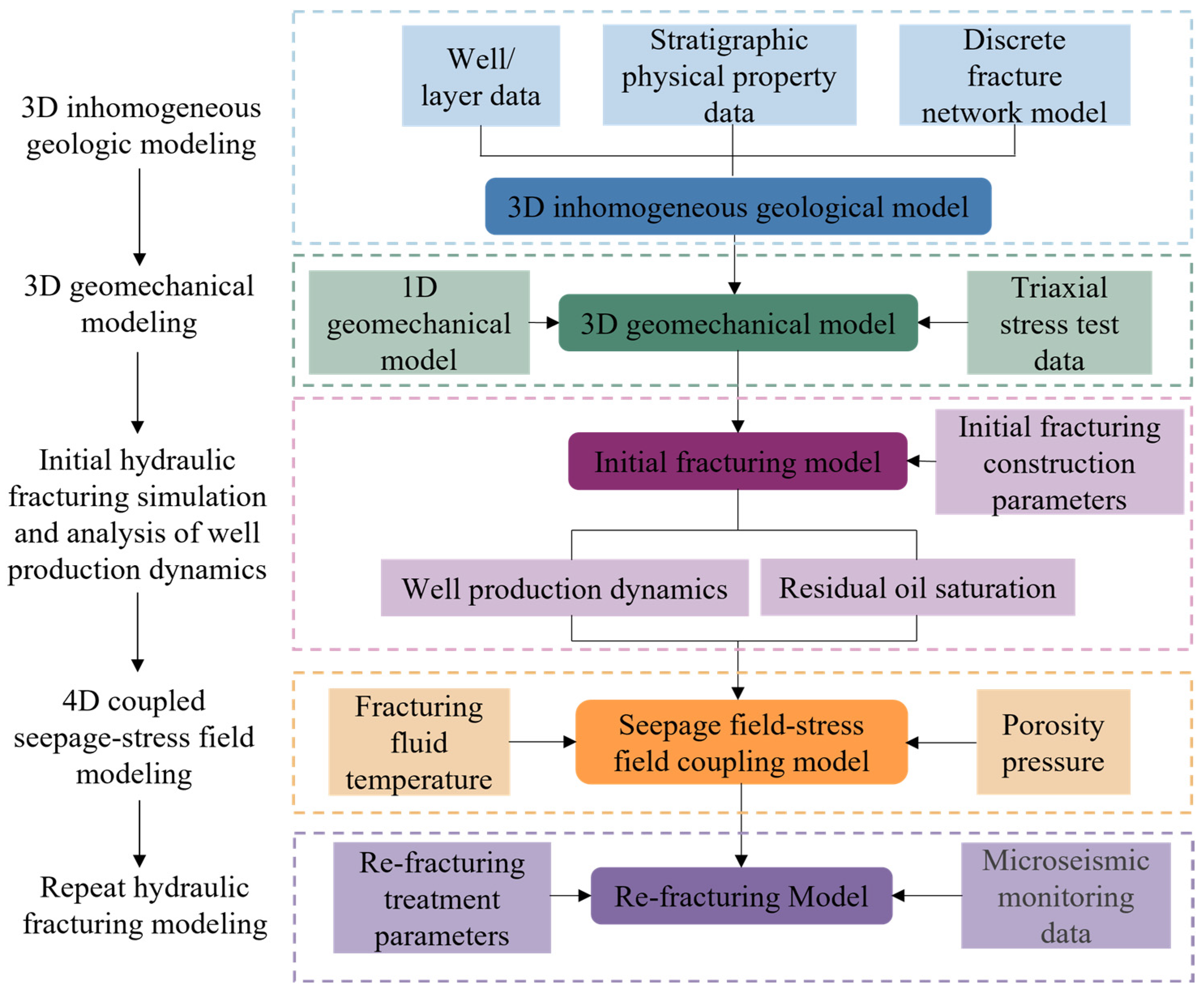
3. Materials and Methods

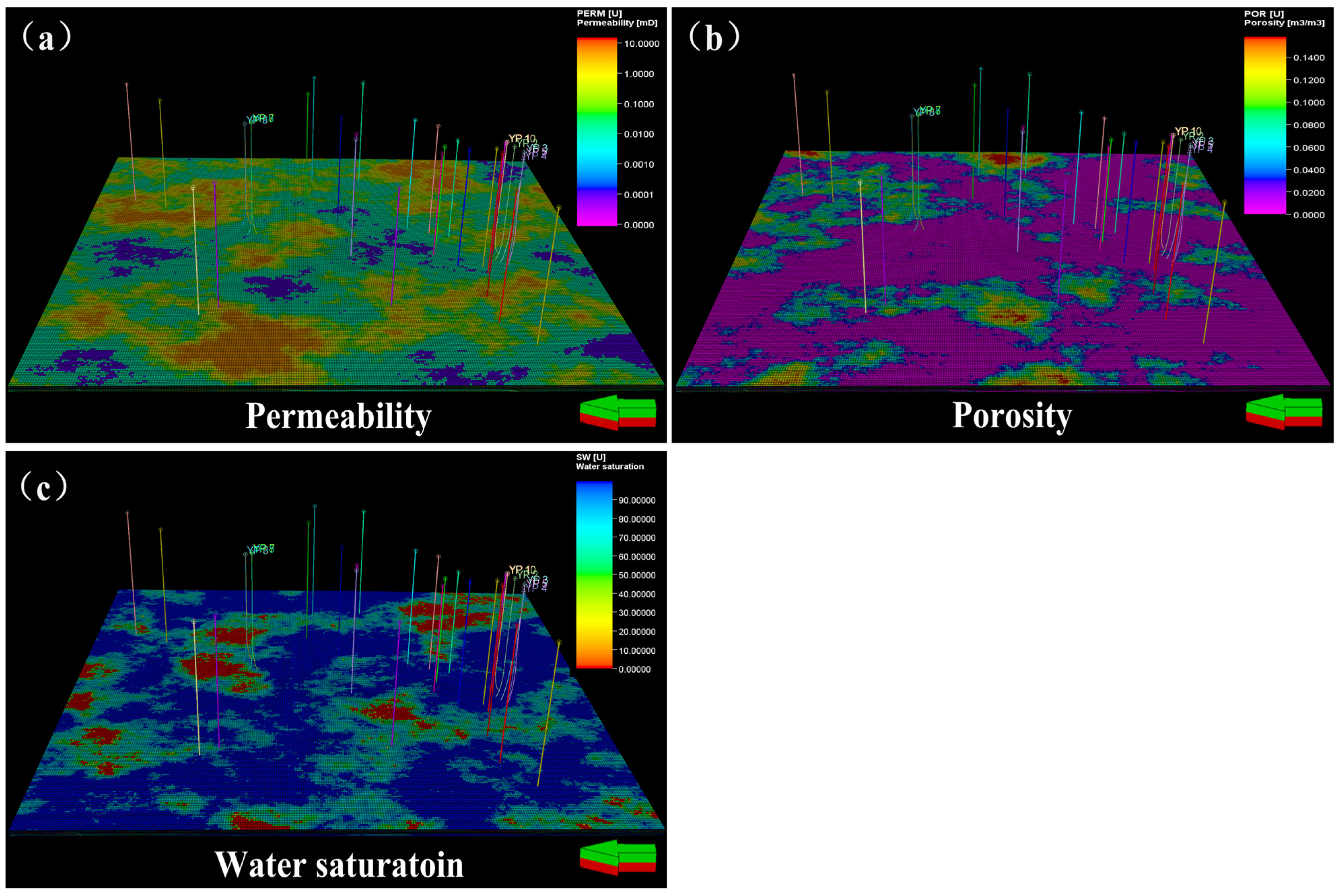
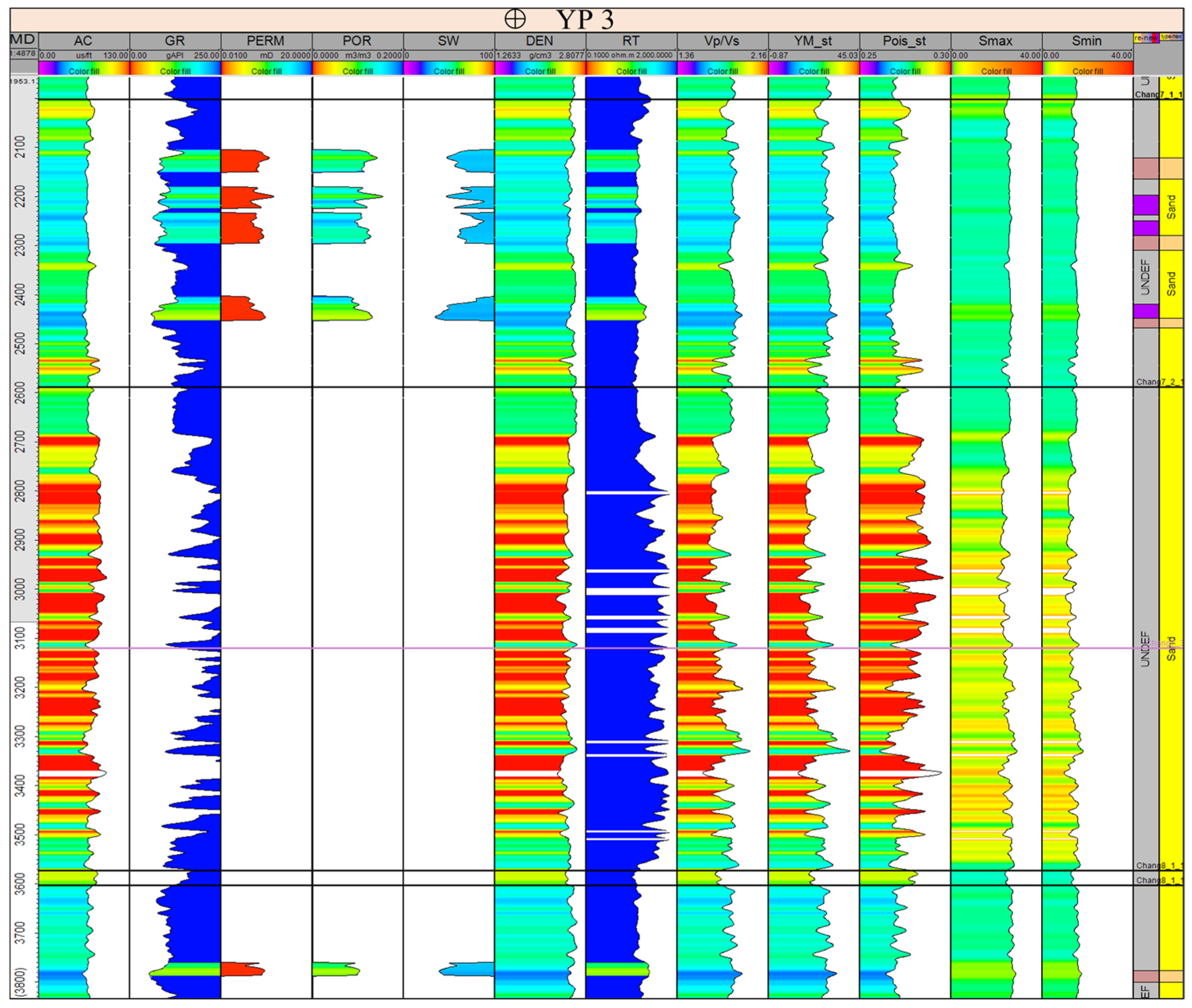
3.1. Three-Dimensional Heterogeneous Geological Modeling

Logging curves and layering models are used to create three-dimensional property models of porosity, permeability, oil saturation, and other characteristics for the matrix model. To get the matrix model, the models are upscaled using several upscaling techniques. The multi-scale matrix model uses outcrop, core, and imaging logging to determine the kind and development mode of fractures. To create fracture models at various scales, the position, inclination, and length of the fractures are counted and included in the model. The porosity and permeability models of the fractures are then obtained by upscaling these models using a variety of techniques. To create a three-dimensional heterogeneous geomechanical model, the aforementioned matrix and fracture models were combined into a single grid system. To create a three-dimensional heterogeneous geomechanical model, the matrix and fracture models were combined into a single grid system [24,25].

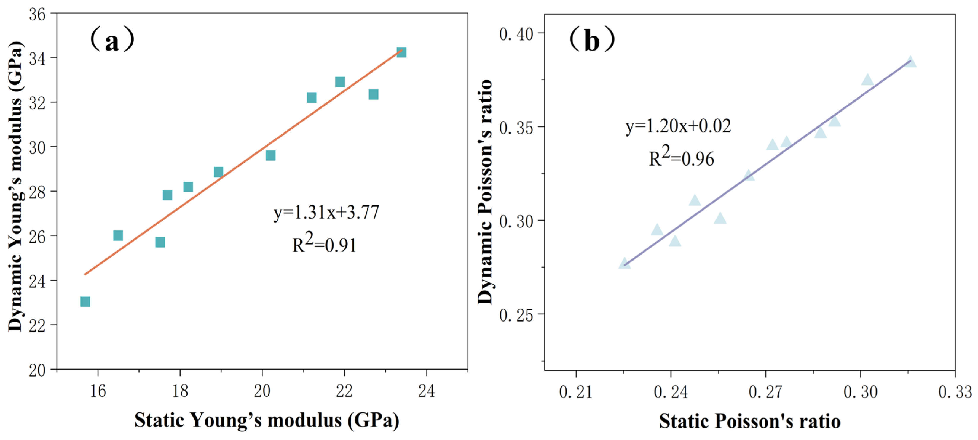
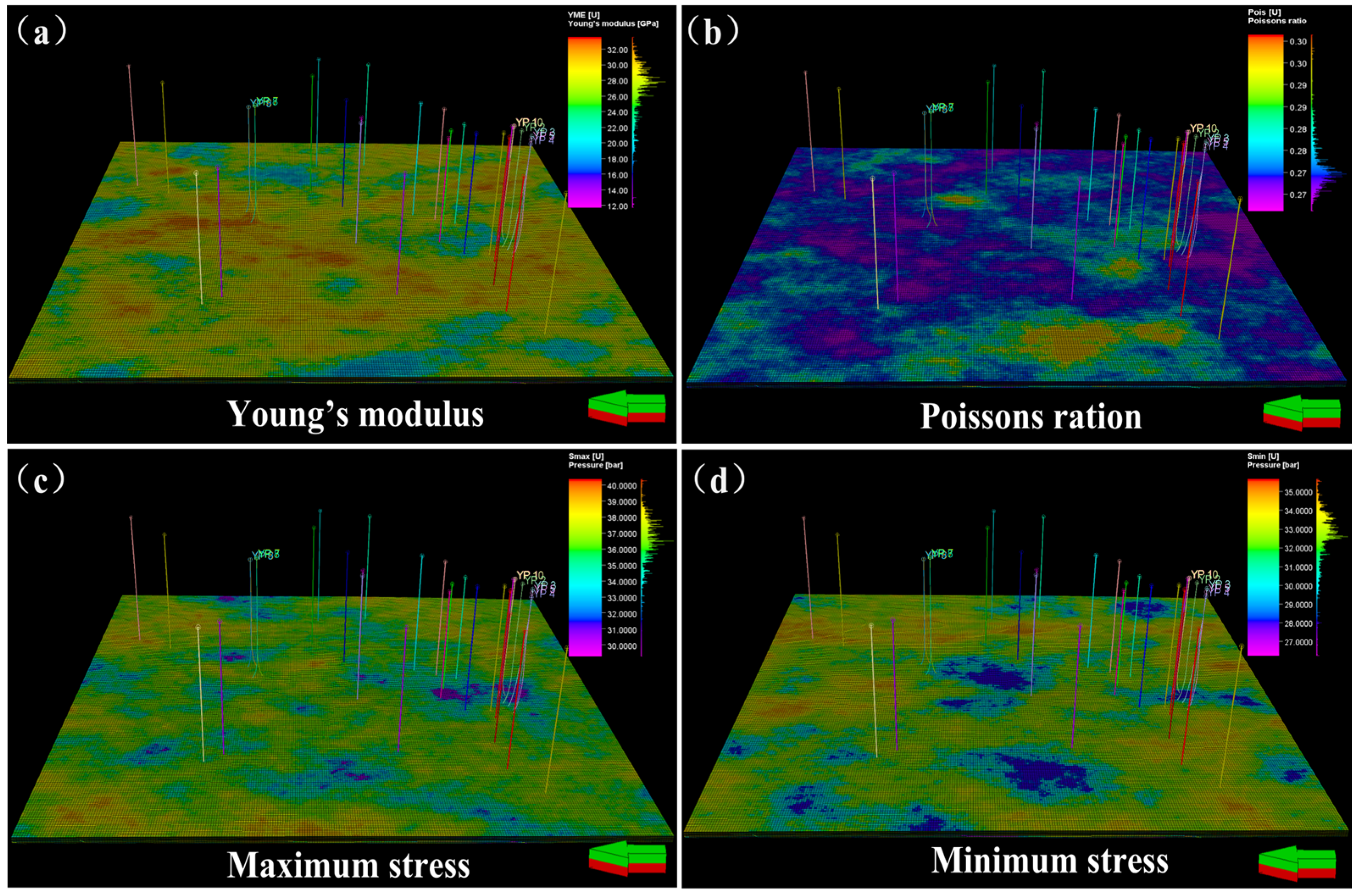
3.2. Three-Dimensional Geomechanical Modeling

A 1D geomechanical model was first created based on the geologic model to depict the deformation resistance of rocks in line with the theory of elastic mechanics. Density logging and acoustic logging were used to determine the elastic constants of rocks, such as Poisson’s ratio and Young’s modulus [26]. Zheng [27] et al. used Equations (1) and (2) to determine the dynamic Young modulus (YME) and the dynamic Poisson ratio (PR).

$$YME=\rho V_S^2{\displaystyle \frac{{3V}_P^2-{4V}_S^2}{V_P^2-V_S^2}}$$

(1)

$$PR={\displaystyle \frac{V_P^2-{2V}_S^2}{{2(V}_P^2-V_S^2)}}$$

(2)

where $\rho$ is the packing density, g/cm²; $YME$ is the dynamic Young’s modulus, MPa; $PR$ is the dynamic Poisson’s ratio.

However, as shown in Figure 3 from sonic logging and triaxial stress test data, dynamic YME and PR must be converted to static YME and PR [28].

The tension that the overlying formation loads (also known as the overlaying formation pressure) place on the reservoir at a specific depth h is represented by the vertical stress ($S_V$). Equation (3) is used to determine the vertical stress [29]. According to the porous elasticity theory, Ranjbar suggested utilizing Equation (4) to determine the maximum horizontal principal stress (${SH}_{max}$) and the acoustic log data to determine the minimum horizontal principal stress (${Sh}_{min}$) [30].

$$S_V={\int }_0^h\rho \left(h\right)g dh$$

(3)

$${SH}_{max}={\displaystyle \frac{PR}{1-\mathrm{P}\mathrm{R}}}{S}_V+{\displaystyle \frac{1-2\mathrm{P}\mathrm{R}}{1-\mathrm{P}\mathrm{R}}}{\alpha P}_P+\alpha P_P+{\displaystyle \frac{YME}{1-{PR}^2}}{\epsilon }_H+{\displaystyle \frac{\mathrm{P}\mathrm{R}.YME}{1-{PR}^2}}{\epsilon }_h$$

(4)

$${Sh}_{min}={\displaystyle \frac{PR}{1-\mathrm{P}\mathrm{R}}}{S}_V+{\displaystyle \frac{1-2\mathrm{P}\mathrm{R}}{1-\mathrm{P}\mathrm{R}}}{\alpha P}_P+\alpha P_P+{\displaystyle \frac{YME}{1-{PR}^2}}{\epsilon }_h+{\displaystyle \frac{\mathrm{P}\mathrm{R}.YME}{1-{PR}^2}}{\epsilon }_H$$

(5)

In this case, the formation pore fluid pressure can be obtained from Eaton’s equation using sonic logging and resistivity logging estimation.

$$P_P=S_V-{\left({\displaystyle \frac{{DT}_n}{DT}}\right)}^{\alpha }(S_V-p_h)$$

(6)

where $S_V$ is vertical stress, MPa; $h$ is the depth of the target layer, m; ${SH}_{max}$ is the maximum horizontal principal stress, MPa; ${Sh}_{min}$ is the minimum horizontal principal stress, MPa; $\alpha$ is the Biot coefficient; $P_P$ is the pore fluid pressure of the formation, MPa; ${\epsilon }_H$, ${\epsilon }_h$ are the strains in the direction of ${SH}_{max}$ and ${Sh}_{min}$; $DT$ is the DT is the propagation time of the acoustic wave at normal, s; ${DT}_n$ is the acoustic wave propagation time obtained in compression logging, s; and $p_h$ is the hydrostatic pressure, MPa.

By computing the property differences in three-dimensional space, the 3D geomechanical model is produced based on the geologic model and the 1D geomechanical model. By contrasting the attribute results and variations in 3D space with the experimental data from the triaxial stress test, the accuracy of the 3D model is confirmed. The research work area’s 3D geomechanical characteristics, such as YME, PR, and other geomechanical parameters, are acquired [31].

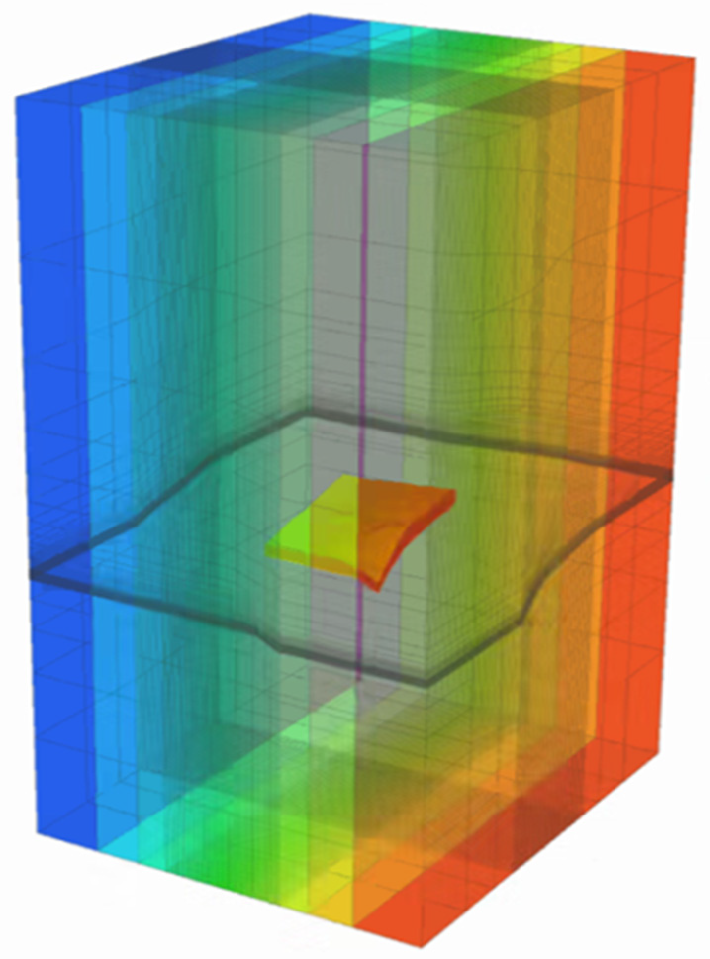
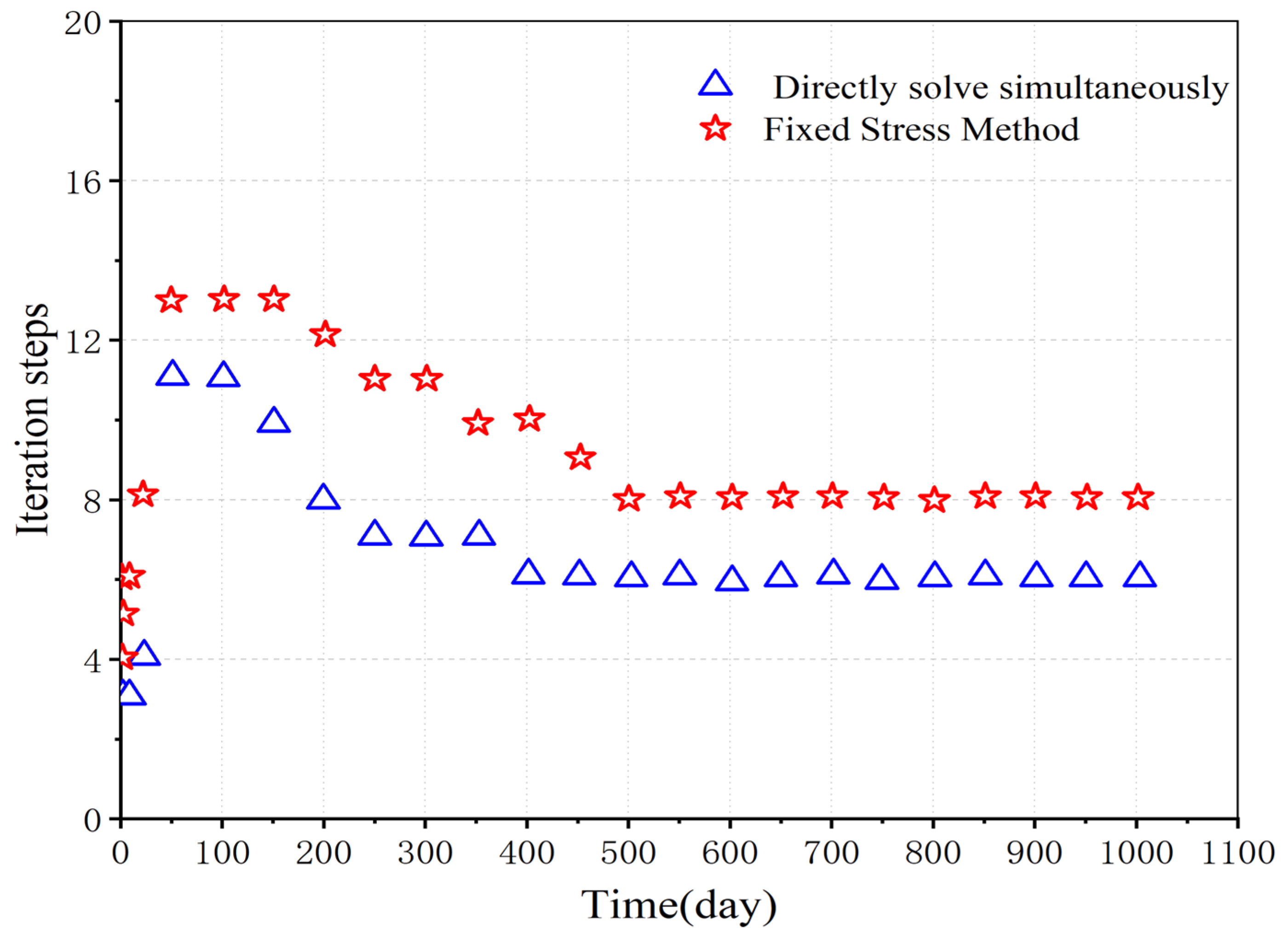
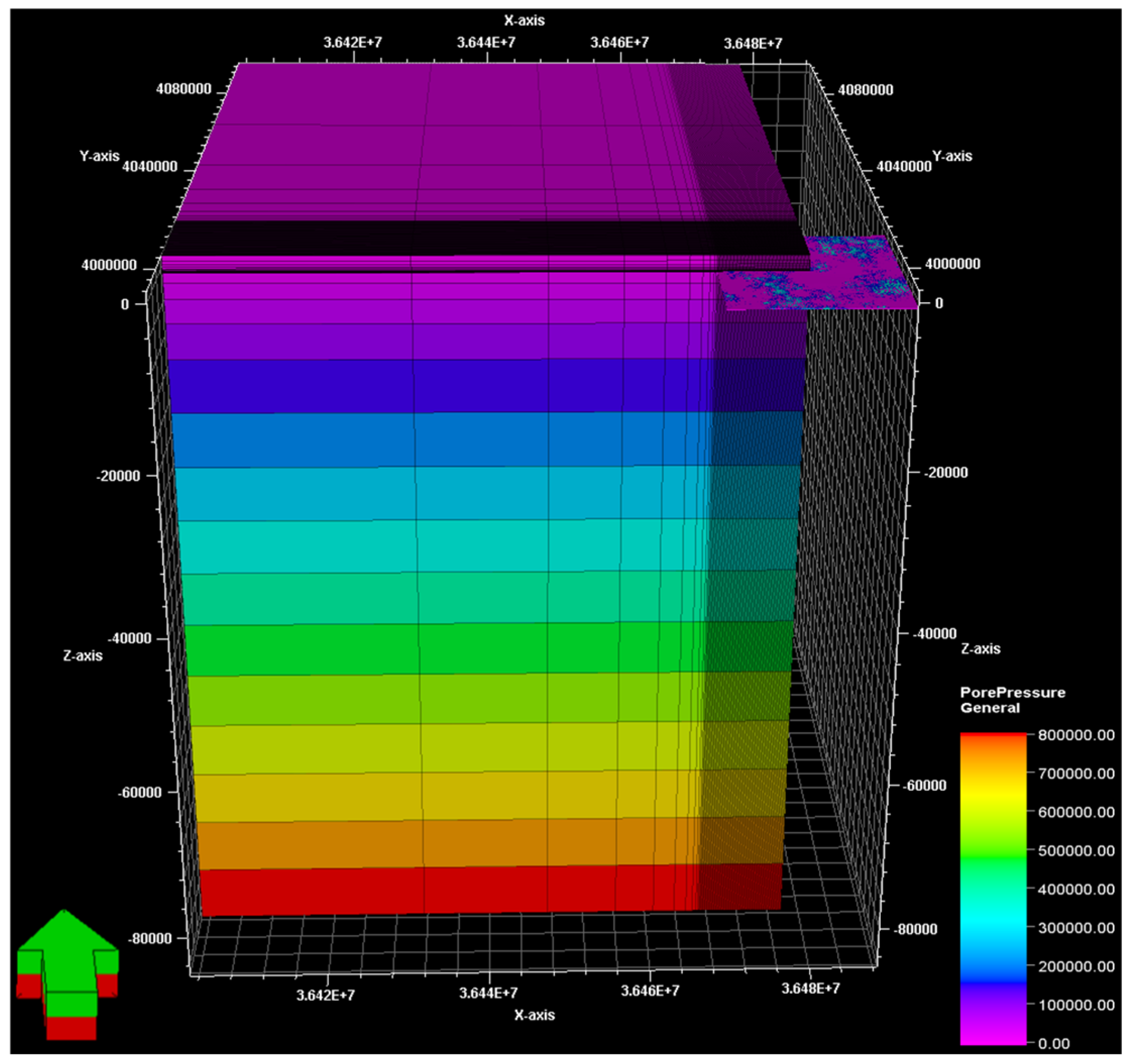
3.3. Coupled Seepage Field-Stress Field Modeling

A multi-field fully coupled simulation method is developed based on porous elasticity theory, the finite element method, and the consideration of the microscopic seepage mechanism of shale oil by combining the seepage equations in the porous medium with the equilibrium equations of the rock and the eigen equations. This approach is intended to address the issues of dredging and the stress reorientation of residual oil following initial fracture recovery. According to the notion, the rock skeleton is elastic, linear, and conforms to the Biot porous elasticity theory [32]. Shale oil has an adsorption impact, and the combined effects of pore pressure and effective stress, as well as the combined effects of fracture opening and closing, affect permeability [33].

The 3D constitutive equation based on Biot’s effective stress concept has the following component form:

$$\left\{\begin{array}{c}{\sigma }_{xx}=C_{11}{ϵ}_{xx}+C_{12}{ϵ}_{yy}+C_{13}{ϵ}_{zz}+C_{14}{\gamma }_{xy}+C_{15}{ϵ}_{yz}+C_{16}{ϵ}_{xy}\\ {\sigma }_{yy}=C_{21}{ϵ}_{xx}+C_{22}{ϵ}_{yy}+C_{23}{ϵ}_{zz}+C_{24}{\gamma }_{xy}+C_{25}{ϵ}_{yz}+C_{26}{ϵ}_{xy}\\ {\sigma }_{zz}=C_{31}{ϵ}_{xx}+C_{32}{ϵ}_{yy}+C_{33}{ϵ}_{zz}+C_{34}{\gamma }_{xy}+C_{35}{ϵ}_{yz}+C_{36}{ϵ}_{xy}\\ {\tau }_{xy}=C_{41}{ϵ}_{xx}+C_{42}{ϵ}_{yy}+C_{43}{ϵ}_{zz}+C_{44}{\gamma }_{xy}+C_{45}{ϵ}_{yz}+C_{46}{ϵ}_{xy}\\ {\tau }_{yz}=C_{51}{ϵ}_{xx}+C_{52}{ϵ}_{yy}+C_{53}{ϵ}_{zz}+C_{54}{\gamma }_{xy}+C_{55}{ϵ}_{yz}+C_{56}{ϵ}_{xy}\\ {\tau }_{zx}=C_{61}{ϵ}_{xx}+C_{62}{ϵ}_{yy}+C_{63}{ϵ}_{zz}+C_{64}{\gamma }_{xy}+C_{65}{ϵ}_{yz}+C_{66}{ϵ}_{xy}\end{array}\right.$$

(7)

where $\sigma$ is the stress tensor; $C$ is the elastic stiffness matrix; and $ϵ$ is the strain tensor.

The stress field’s equilibrium equation, which takes the seepage volume force into account, is provided by

$$\left\{\begin{array}{c}{\displaystyle \frac{{\partial \sigma }_{xx}}{{\sigma }_x}}+{\displaystyle \frac{{\partial \tau }_{xy}}{{\sigma }_y}}+{\displaystyle \frac{{\partial \tau }_{xz}}{{\sigma }_z}}-\alpha {\displaystyle \frac{\partial p}{{\sigma }_x}}=0\\ {\displaystyle \frac{{\partial \tau }_{yx}}{{\sigma }_x}}+{\displaystyle \frac{{\partial \sigma }_{yy}}{{\sigma }_y}}+{\displaystyle \frac{{\partial \tau }_{yz}}{{\sigma }_z}}-\alpha {\displaystyle \frac{\partial p}{{\sigma }_y}}=0\\ {\displaystyle \frac{{\partial \tau }_{zx}}{{\sigma }_x}}+{\displaystyle \frac{{\partial \tau }_{zy}}{{\sigma }_y}}+{\displaystyle \frac{{\partial \sigma }_{zz}}{{\sigma }_z}}-\alpha {\displaystyle \frac{\partial p}{{\sigma }_z}}=0\end{array}\right.$$

(8)

The compatibility equation, or the relationship between the displacement field and the strain tensor, is [34]:

$$\mathrm{Displacement} \mathrm{field} \mathit{U}=(u,v,w)$$

(9)

$$\mathrm{Strain}\text{-}\mathrm{displacement} \mathrm{relationship} \mathit{\epsilon }={\displaystyle \frac{1}{2}}\left(\mathbf{\nabla }\mathbf{U}+{\left(\mathbf{\nabla }\mathbf{U}\right)}^{\mathrm{T}}\right)$$

(10)

Component form of the compatibility equation:

$$\left\{\begin{array}{c}{\epsilon }_{xx}={\displaystyle \frac{\partial u}{\partial x}},{\epsilon }_{yy}={\displaystyle \frac{\partial u}{\partial y}}, {\epsilon }_{zz}={\displaystyle \frac{\partial u}{\partial z}} \\ {\gamma }_{xy}={\displaystyle \frac{\partial u}{\partial y}}+{\displaystyle \frac{\partial v}{\partial x}}, {\gamma }_{yz}={\displaystyle \frac{\partial v}{\partial z}}+{\displaystyle \frac{\partial w}{\partial y}},{\gamma }_{zx}={\displaystyle \frac{\partial w}{\partial x}}+{\displaystyle \frac{\partial u}{\partial z}} \end{array}\right.$$

(11)

The microscopic seepage mechanism of shale oil in combination with Darcy’s law, the impact of pore changes on permeability, and the response of stress variations on fluid flow must all be taken into account when discussing seepage.

Darcy’s seepage law governs how pore fluids leak through porous media:

$$\left\{v\right\}=-\left[K\right]\left\{\nabla h\right\}$$

(12)

Continuity equations for pore fluids:

$${\nabla }^T\left\{v\right\}-Q={\left\{m\right\}}^T\alpha {\displaystyle \frac{\partial \epsilon }{\partial t}}+\left[{\displaystyle \frac{\left(n-1\right)}{K_s}}+{\displaystyle \frac{n}{K_w}}-{\displaystyle \frac{k_T}{{\left(K_s\right)}^2}}\right]{\displaystyle \frac{\partial p}{\partial t}}$$

(13)

Ordinary differential equation form:

$$\left[\begin{array}{cc}0& 0\\ 0& \left[KP\right]\end{array}\right]\left\{\begin{array}{c}\left\{u\right\}\\ P\end{array}\right\}+\left[\begin{array}{cc}\left[K\right]& \left[C\right]\\ {\left[C\right]}^T& CP\end{array}\right]{\displaystyle \frac{d}{dt}}\left\{\begin{array}{c}\left\{u\right\}\\ P\end{array}\right\}=\left\{\begin{array}{c}\left\{dF/dt\right\}\\ \left\{Q\right\}+\left\{G\right\}\end{array}\right\}$$

(14)

The updated porosity and permeability equations are [35]:

$$\varnothing ={\displaystyle \frac{{\varnothing }_0-∆\varnothing }{1-∆\varnothing }} \left[K\right]=\left[K_0\right]{\displaystyle \frac{{\varnothing }^3/{\left(1-\varnothing \right)}^2}{{\varnothing }_0^3/{\left(1-{\varnothing }_0\right)}^2}}$$

(15)

The equations for the seepage field and stress field are completely coupled. In Figure 4, the seepage field and stress field are implicitly iteratively connected between the flow and solid, which are simulated independently using a dual mesh [36]. Although the geomechanical dual mesh can reduce the boundary effects and make the mechanical boundary conditions more realistic, the meshes are created independently for these two physical problems, and a coarser mesh can be utilized for the solids on the outside of the fluid flow zone [37,38].

The black oil model’s three-component equation in general form is as follows:

$$Q_i={\displaystyle \frac{\partial \left({\sum }_j\mathrm{\varnothing }{\rho }_j{S}_j{x}_j^i\right)}{\partial t}}+\left({\sum }_j\mathrm{\varnothing }{\rho }_j{S}_j{x}_j^i\right){\displaystyle \frac{\partial {\epsilon }_v}{\partial t}}\nabla \left(-{\sum }_j{x}_j^i{\displaystyle \frac{{\rho }_j{k}_{rj}}{u_j}}\mathit{K}\left({\nabla P}_j-{\rho }_j\mathrm{g}\right)\right)$$

(16)

In situ stress equation:

$$\nabla \left(C_{dr}:\epsilon -b{P}_f\delta \right)+{\rho }_b\mathrm{g}=0$$

(17)

Corrections to the porosity model were made using the fixed stress method:

$$\delta \varnothing ={\displaystyle \frac{\left(b-\varnothing \right)}{K_s}}\delta P+\left(b-\varnothing \right)\delta {\epsilon }_V$$

(18)

$$\mathrm{Included} \mathrm{among} \mathrm{these} \delta {\epsilon }_v={\displaystyle \frac{b}{K_{dr}}}\delta P+{\displaystyle \frac{1}{K_{dr}}}\delta {\sigma }_v$$

where: ${\sigma }_v$ is the Newton step, constant; $\delta {\sigma }_v$ is the stress, constant 0.

Figure 4. Flow–solid “dual mesh” discretization. Different colors represent different positions with respect to the core model.

Figure 4. Flow–solid “dual mesh” discretization. Different colors represent different positions with respect to the core model.

In the direct coupled solution, fixed stress method iteration convergence speed is faster than the two-way iteration technique, as shown in Figure 5, but the number of iterations is only slightly increased, and the size of the matrix of a single solution is greatly reduced [37]. It is used to address increasingly complicated problems that are closer to the real model in the field since it greatly increases the stability and iteration speed of connected simulation.

Figure 5. Comparison of two fully coupled iterative methods.

Figure 5. Comparison of two fully coupled iterative methods.

The discrete form of the fully coupled term of the multiphase flow equation is [38]:

$${\displaystyle \frac{\partial \left({\sum }_j\mathrm{\varnothing }{\rho }_j{S}_j{x}_j^i\right)}{\partial t}}+\left({\sum }_j\mathrm{\varnothing }{\rho }_j{S}_j{x}_j^i\right){\displaystyle \frac{\partial {\epsilon }_v}{\partial t}}\approx {\displaystyle \frac{1_i}{∆t}}{\left\{\left({\sum }_j\mathrm{\varnothing }{\rho }_j{S}_j{x}_j^i\right)+\left(1+∆{\epsilon }_v\right)\right\}}^n-{\displaystyle \frac{1}{∆t}}{\left({\sum }_j\mathrm{\varnothing }{\rho }_j{S}_j{x}_j^i\right)}^{n-1}$$

(19)

3.4. Refracturing Numerical Simulations

To attempt to solve the induced influence of initial fractures on the fracture propagation of future fractures, we built a numerical simulation system for the entire refracturing operation. First, the system was based on a heterogeneous geomechanical model, coupling the in situ stress field and pore pressure field of the initial fracturing, integrating the residual fracture network formed by the initial fracturing [39].

A 3D fracture dynamic initiation model is established using the modified Hossain fracture initiation criterion, considering fluid–solid coupling. The stress intensity factor at the fracture tip is solved using the finite element method, and a synergistic extension model of the artificial-natural fracture system is constructed by adopting the contact mechanics model to characterize the fracture interference, utilizing the theory of fracture mechanics to quantify the critical conditions of the activation of the natural fracture, and dynamically correcting the fracture extension trajectory through the assimilation of the is the microseismic monitoring data in real-time. Fracture extension trajectories with dynamic correction. Equations (20) and (21) rigorously characterize the power-law rheological properties of the fracturing fluid flow regime [40,41], which is specifically decoupled into a Darcy seepage regime in the proppant-filled zone and a turbulent flow regime within the main fracture. The degree of shear rarefaction is represented by n = 0.35–0.65, while the rate of viscosity decay is controlled by K = 0.6 − 1.0 Pa·sⁿ.

$${\displaystyle \frac{d∆p}{dx}}={\displaystyle \frac{R{\nu }^n}{(\mathrm{n}+2){\omega }^{n+1}}}$$

(20)

$$R={\displaystyle \frac{2K{\left(2m\right)}^n(n+2)}{{\left[{(4/\pi )}^m\varphi \right]}^n}} m={\displaystyle \frac{2\mathrm{n}+1}{2n}}$$

(21)

$${\varphi }^n\simeq 1-0.41n^{0.61}$$

(22)

where $n$ is the power rate index; K is the consistency index; $\varphi$ is the flow coefficient; $\nu$ is the flow velocity; $\omega$ is the average seam width.

It is evident from the UFM model that the fracture tip extends in a peaked plane. The average flow rate in the crack cross section can be calculated using Poiseuille’s equation of flow as follows [42]:

$$\overline{q}=-{\displaystyle \frac{H{\omega }^2}{12\mu h}}\nabla q$$

(23)

The relationship between the average fracture opening and the characteristic width is satisfied:

$$\overline{\omega }={\displaystyle \frac{\omega H}{h}}$$

(24)

The quality equation for controlling fracture propagation is as follows [43]:

$${\displaystyle \frac{\partial q}{\partial S}}+{\displaystyle \frac{\partial \left(H_{fl}\omega \right)}{\partial t}}+q_L=0 (q_L={\displaystyle \frac{2h_L{C}_L}{\sqrt{t-T_0\left(s\right)}}},t>0)$$

(25)

where $H$ is the height of the fracture, m; $q$ is the local flow rate inside the hydraulic fracture along any secondary joint; $q_L$ is the leak-off volume into the rock matrix through the hydraulic fracture wall per unit length; $h_L$ is the height of the leak-off zone; $C_L$ is the total leak-off coefficient; $H_{fl}$ is the local height of the fracture occupied by the open fluid; $T_0\left(s\right)$ is the time at which each unit of the fracture is first exposed to the fracturing fluid.

Furthermore, the entire volumetric network, which includes the fracture, perforation, and wellbore, should satisfy the overall volume balance Equation (26) in which the volume of fracturing fluid pumped by the fracturing fleets equals the sum of the volumes filled in the volumetric network’s fracture and the volume of the fracturing fluid matrix lost by leak-off under pressure [44].

$${\int }_0^{t}Q\left(t\right)dt={\int }_0^{L\left(t\right)}h\left(s,t\right)\overline{w}(s,t)ds+{\int }_{H_L}{\int }_0^t{\int }_0^{L_t}{2u}_L ds dt {dh}_L$$

(26)

where $u_L$ is the leak-off loss velocity; $\overline{w}$ is the position s = s (x, y).

4. Results

4.1. Three-Dimensional Heterogeneous Geological Model

The stratification model of four sublayers was established in the Chang 7 Formation based on the drilling stratification data at the research work area. These four sublayers are Chang 711, 712, 721, and 722. The 3D space was interpolated using the algorithm of the synergistic Kriging-Gaussian stochastic function, and a 3D heterogeneous geological model was established. According to the modeling results, the established work area is 11 km × 10 km, including 1,276,560 grids, the model precision is 50 m × 50 m, and each grid is 2–8 m in height. The estimated reservoir permeability, porosity, and water saturation are 10.32%, 0.2 mD, and 43%, respectively, as shown in Figure 6.

4.2. Three-Dimensional Geomechanical Model

To create a 1D heterogeneous in situ stress model for the YP 3 well, the rock mechanics parameters are computed and transformed into action statics based on the transverse wave and density logging curves and the rock mechanics formula. The YME, PR, and maximum and minimum horizontal principal stresses for YP 3 well are shown in Figure 7. Rock mechanic modeling, with average values of 27 GPa, 0.27, and 37.2 MPa, 31.5 MPa, respectively, was voted.

Under the limitations of the 3D geological model, a 3D geomechanical model is created based on the stress profile of a single well. The reservoir’s 3D geomechanical grids, as well as the lateral, overburden, and underlying grids, are configured to maintain a constant far-field stress state at the model’s boundaries, necessary to prevent stress concentration and uniform loading of the boundary loads. Figure 8 illustrates the extension of the geomechanical grid outward with equal scale fracture propagation; the width-to-depth ratio of the 1/4 portions of the model is 2:1, and the grid accuracy is 236 × 289 × 50. With 3,410,200 grids and 3,505,230 nodes, one quarter of the geomechanical grid is finished. According to the study, the characteristics of the 3D geomechanical model include the following: the maximum horizontal principal stress data in Figure 9c are primarily in the range of 28–42 MPa, with an average value of 37 MPa; the minimum horizontal principal stress data in Figure 9d are primarily in the range of 26–36 MPa, with an average value of 37 MPa; and the Young’s modulus data in Figure 9a are primarily in the range of 18–34 GPa, with an average value of 27 GPa; the Poisson’s ratio data in Figure 9b are primarily in the range of 0.26.03, with an average value of 0.268.26–36 MPa, with 32.5 MPa being the average.

4.3. Analysis of Initial Fracturing, Fracture Propagation, and Oil Well Production Performance

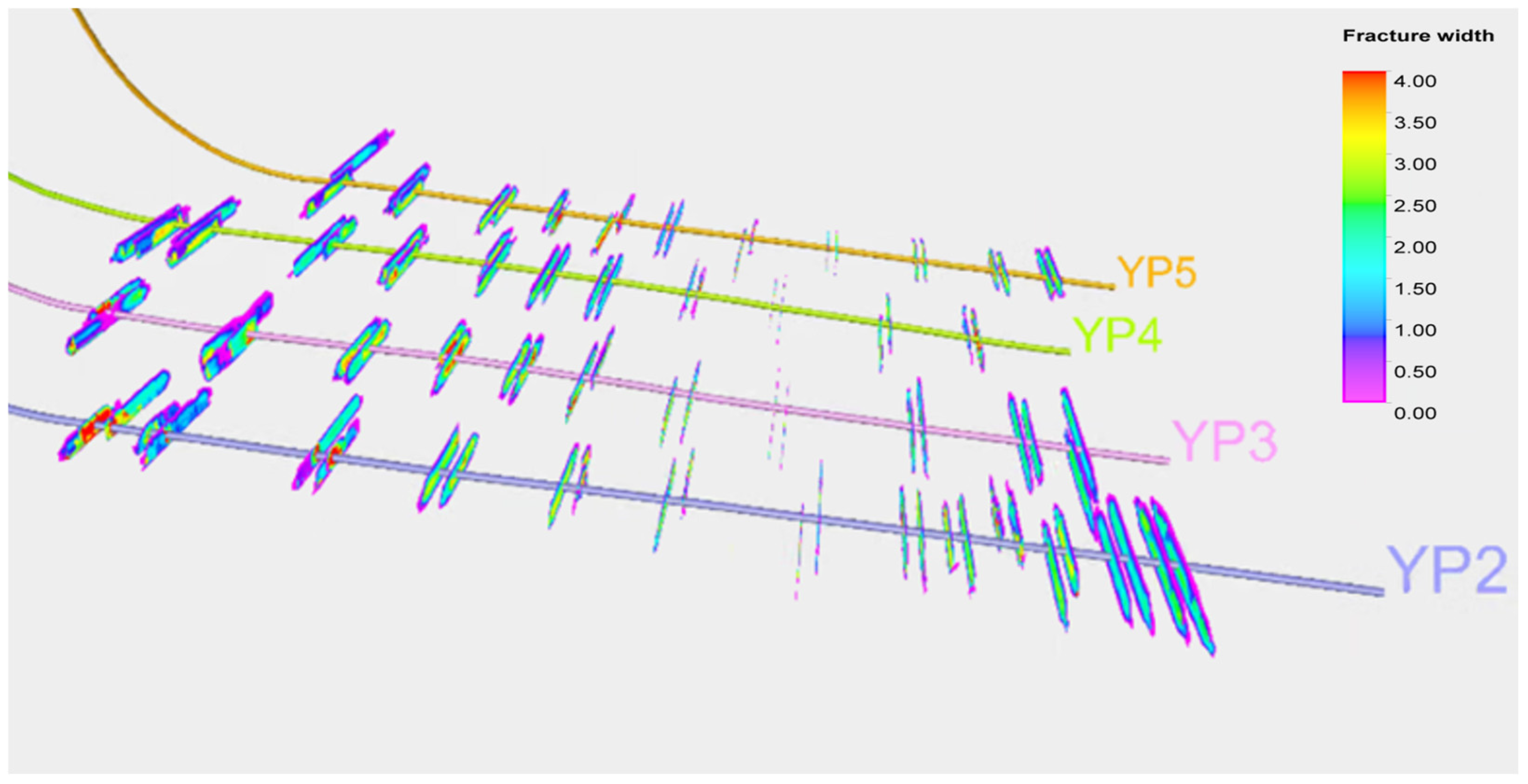
4.3.1. Fracture Propagation of Initial Fracturing

The entire horizontal well is divided into 11 stages and 22 clusters for hydraulic fracturing, as shown in

Table 1. Initial fracturing design and parameters.

Initial Fracturing Construction Parameter Design
Construction parameters	stage 1		stage 2		stage 3		stage 4		stage 5		stage 6		stage 7		stage 8		stage 9		stage 10		stage 11
	Tubing	Casing	Tubing	Casing	Tubing	Casing	Tubing	Casing	Tubing	Casing	Tubing	Casing	Tubing	Casing	Tubing	Casing	Tubing	Casing	Tubing	Casing	Tubing	Casing
Treatment pressure/MPa	44.8	37.8	39.3	34.5	53.8	34.6	45.4	35.8	48.7	35.5	48.2	31.6	48.1	30.7	44.6	30.1	45	30.9	45.4	24.9	37.9	25.1
Sand volume/m3	45.1		43.7		43.9		43.4		43.7		43.5		43.7		44.5		44.3		44		43.6
Sand Concentration kg/m3	155.1		165		169.2		166.4		163.8		160.7		165.4		170.4		167		160.7		164.4
Rate m3/min	2	4	1.8	4.2	1.8	4.2	1.8	4.2	1.8	4.2	1.8	4.2	1.8	4.2	1.7	4.2	1.8	4.2	2	4	2	4
Pad/m3	82.1	141	42.9	84.1	62.8	112.1	44.1	84.3	45.7	84.1	45.3	82.4	47.5	80.9	51.7	100.8	62.3	123.7	51	88.1	54.6	79.6
slurry/m3	160.7	320.2	124.5	288.2	120.6	283.4	122.8	284.1	126.4	289.8	127.7	292.1	124.4	286.8	117.9	289.8	123.3	289.1	143.3	281.7	140.2	273.6
Flush/m3	15.7	30.7	16.2	35.3	15.4	35.4	33.8	15.4	13.6	30.5	12.9	29.3	13.5	30.2	11.1	28.1	15.2	34.5	13.5	25.5	12	23.7
Total fluid/m3	259.2	466.5	183.6	380.2	198.8	403.5	200.7	357.4	185.7	377.9	185.9	376.4	185.4	371.4	180.7	391.3	200.8	420.3	207.8	368.5	206.8	350.7

. The cumulative volume of sand and fracturing fluid is 484 m³ and 6560 m³, and the average rate is 6 m³/min. The UFM model was used to solve the full coupling problem between the flow of fracturing fluid and the elastic deformation of the fracture in the fracture network. The hydraulic fractures that are generated are primarily simple 3D complex seams, as illustrated in Figure 10. The stress field distribution is uniform, with the half-length of the initial fracturing seams are 56–82 m, the average seam height measuring 56–82 m, the average seam length measuring 56–82 m, the average seam height measuring 18.45 m, and the average conductivity of the fracture is 17.1 D.cm. We established the fracture complexity of initial fracturing as a basis for conducting fracturing.

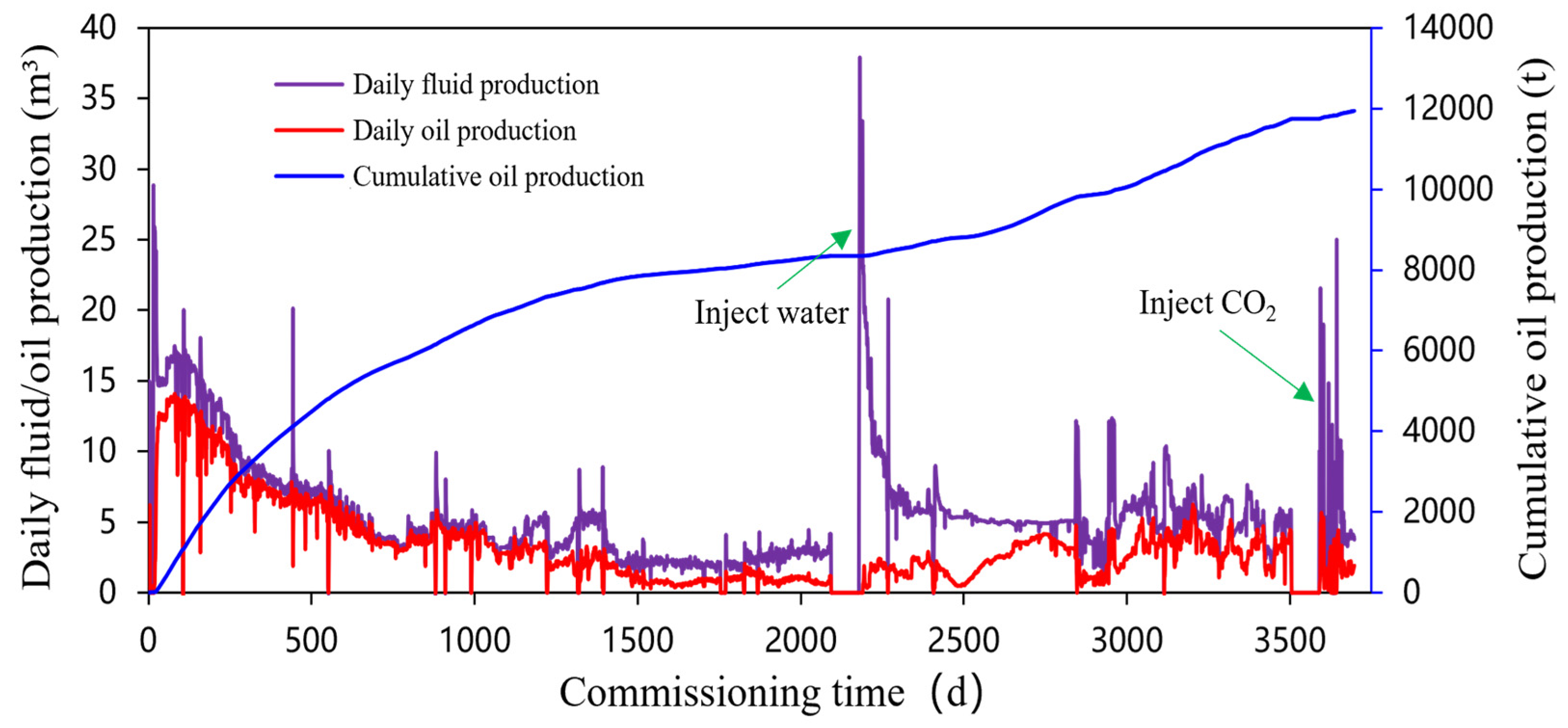
4.3.2. Production Dynamics Analysis of Oil Wells

When the YP 3 well was first placed into production on 29 December 2012, its water content was 64.8%, its initial daily liquid production was 15.98 m³, and its daily oil production was 5.62 t, as shown in Figure 11. On 12 September 2018, the well was injected with water vapor for a throughput experiment. Following the implementation of the measures, the horizontal well’s daily liquid production reached 16.25 m³, its daily oil production reached 1.06 t, and its water content reached 93.5%. The CO₂ injection replenishment experiment was then carried out in August 2022. After a month of production following the measures, the average daily fluid production was 8.61 m³, the daily oil production was 1.95 t, and the water content efficiency of the well was reduced to 76.3%. The well was then shut down for 53 days and opened for 290 days of production. Before refracturing, the daily fluid production was reduced to 3.51 m³, the daily oil production was 1.63 t, and the water content was 49.5%. These results showed that the injected CO₂ was not completely contacted and exchanged with the crude oil.

Based on fracture extension simulation and PEBI grid refinement technology, combined with black oil model three-phase flow simulation and production history fitting, the dynamic evolution law of the pressure field in the YP 3 well is clarified (Figure 12). The initial formation pressure was 15.8 MPa and reached a historical low of 7.8 MPa with continuous extraction before the steam throughput, which occurred in 2018. After the steam throughput (Figure 12d), the formation pressure rebounded to 15.2 MPa, which was close to the original formation pressure, but then started to decline. In 2022, the CO₂ make-up test was implemented, and the pressure increased from 1.4 MPa to 11.4 MPa, but the injected gas and crude oil were not sufficient to create. The contact between the injected gas and the crude oil was insufficient, and the pressure fluctuation was obvious (Figure 12e,f), indicating that the gas diffusion was limited due to the underdevelopment of the fracture network. After 53 days of continuous well smothering, the formation pressure recovered to 85.9% of the original pressure, and the locally high pressure indicated the strong non-homogeneity of the reservoir. In summary, the existing fracture system is difficult to support an efficient CO₂ drive, and repeated fracture modification is required to improve the complexity of the fracture network.

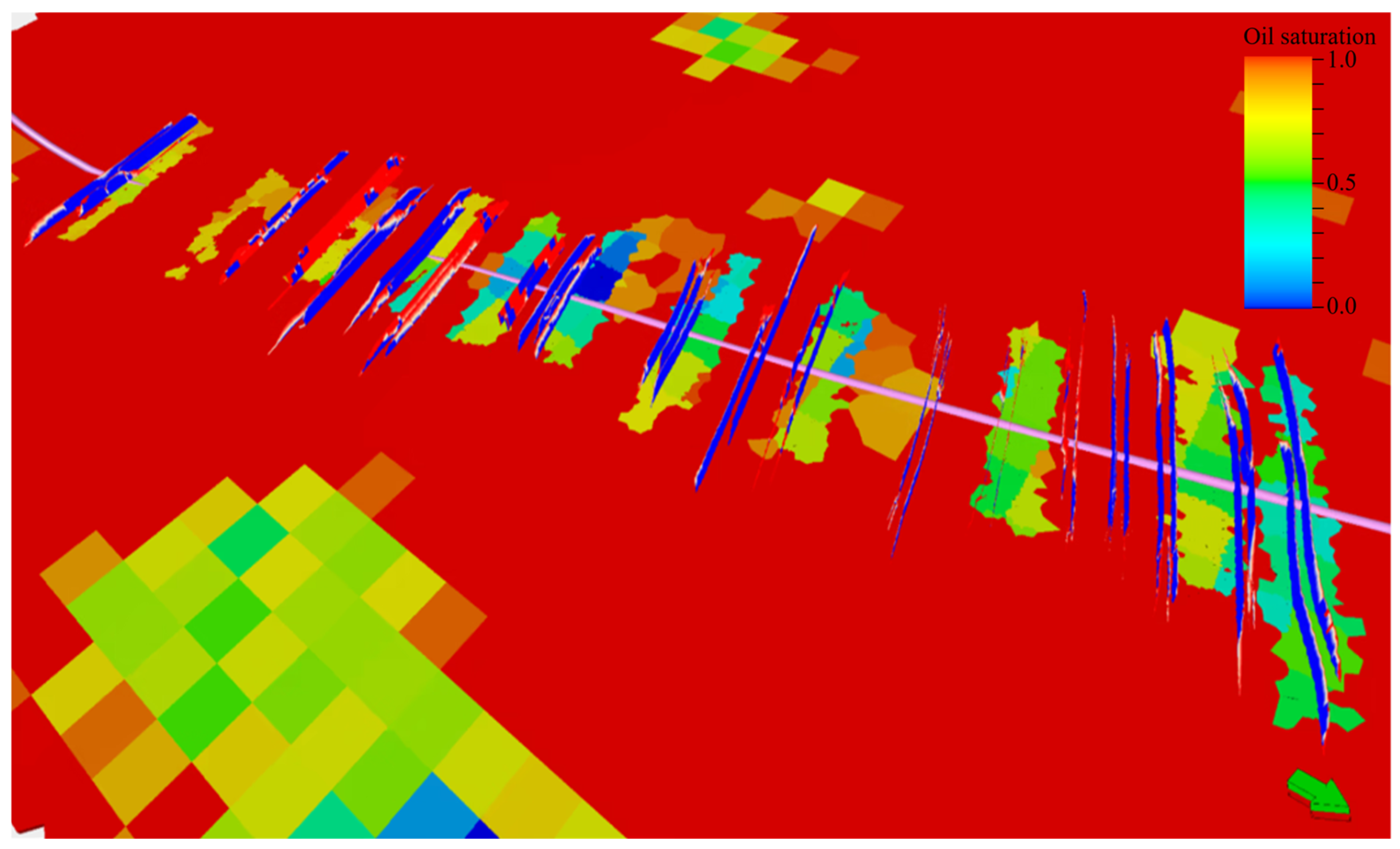
4.3.3. Residual Oil Distribution Pre-Refracturing

Figure 13 illustrates the law of residual oil distribution’s dynamic evolution. While the pressure around the wells gradually fell, the reservoir pressure was high at the start of production in 2013, and the residual oil was mostly confined in the space between the fracture seams. The residual oil between the fracture seams steadily decreased with further depletion (Figure 13b), but the space between the wells continued to be undrained. The pressure surrounding the fracture seams rose with the installation of steam throughput in 2018 (Figure 13c), hastening the recovery of the residual oil in the inter-seam region. Most of the residual oil in the inter-seam area had been extracted by 2024 (Figure 13d); nevertheless, because of the excessive seam spacing and the insufficient half-length of the original fractured seam, a sizeable number of untapped reserves remained in the inter-well area. The cumulative oil production of the YP 3 well is 11,900 tons, according to numerical analysis, and the average drop in oil saturation surrounding the well is 4.74%. These figures closely match the outcomes of multi-field coupled simulation and validate the possibility of the development of the residual oil between fractures. Therefore, it is necessary to optimize the design through fracturing: increase the fracture spacing to 50–70% of the initial fracture, increase the fracturing fluid volume, and ensure that the half-length of the new fracture exceeds that of the initial fracture by 20–30%, to efficiently utilize the remaining oil resources in the inter-well.

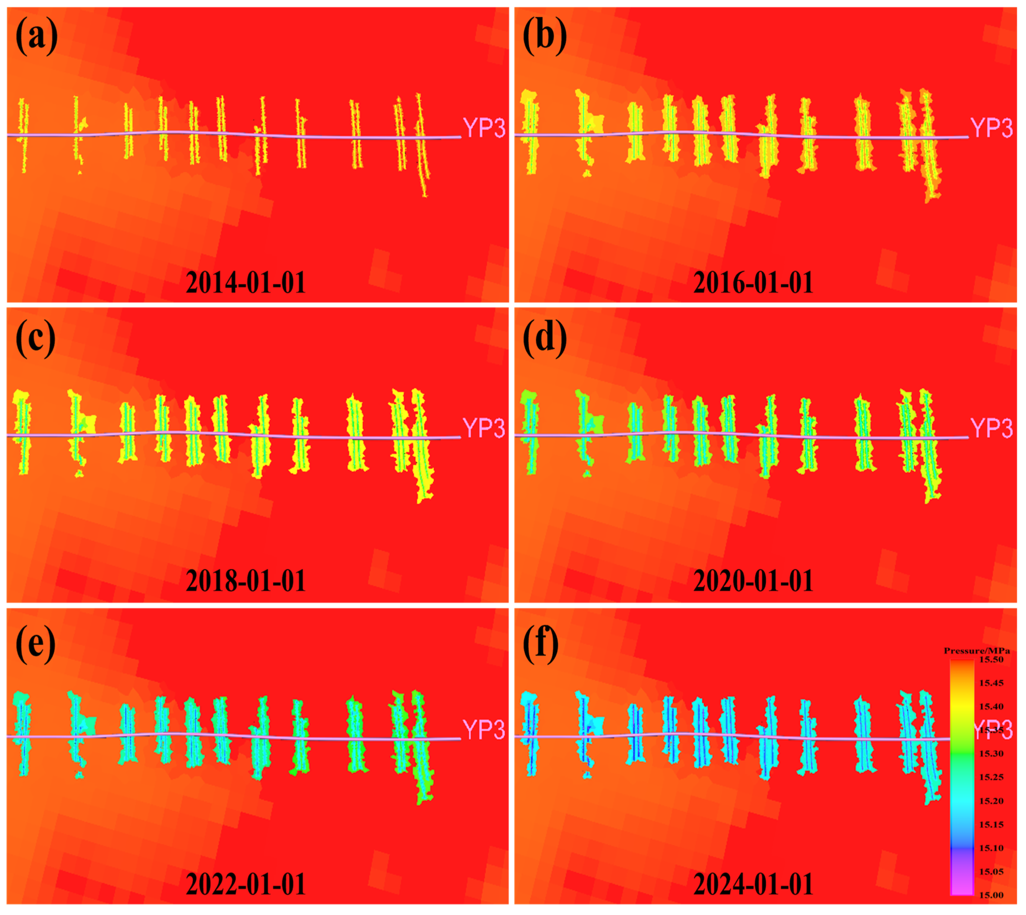
4.4. Four-Dimensional Coupled Seepage–Stress Field Simulation

The coupled seepage–stress field model simulates and computes the stress changes during these initial fracturing periods using the pore pressure, fracturing fluid temperature, and residual oil saturation during various production periods that were obtained from the reservoir simulation previously mentioned. According to the simulation, the in situ stress falls over the production process, and the horizontal primary stress differential has a discernible downward trend, going from 5 MPa to 3 MPa in the initial stage. Furthermore, the minimum principal stress also shows reorientation; as shown in Figure 14, the minimum horizontal principal stress’s maximum reorientation angle is 24°, while its minimum deflection angle is −5° in the opposite direction, suggesting that shifts in stress orientation are only slight. It is difficult to steer fracture fissures during refracturing by deflecting a single stress because the simulation findings in Figure 15 show that the two-way primary stresses across various periods do not reverse. This makes it more difficult for a complex fracture network to form; hence, during repetitive fracturing, it is required to increase the complexity of the fractures using certain fracture blocking procedures.

4.5. Fracture Propagation Simulation During Refracturing

The overlapping geological and engineering parameters in the horizontal section are selected, where the Class II section with slightly poor physical properties in the toe is the main section, and the Class I section in the root is the secondary section. We then carried out refracturing injection hole placement and determined the preferred potential location of 18 stages, with 2–3 perforation clusters per stage, totaling 43 clusters. This was done in conjunction with the distribution of residual oil from the initial fracturing and the analysis of well production dynamics.

4.5.1. Post-Refracturing Simulation

The UFM, which calculates the stress field that causes fracture propagation using a coupled seepage–stress field model, is the basis for simulating re-fracture crack extension. The fracture extension criterion, which is determined iteratively for each node of the extension from fracture initiation and the interplay between hydraulic and natural fractures, makes it possible to simulate 3D fractures [45,46,47]. To mimic refracturing fracture extension, the refracturing construction parameters are entered based on the reconstructed seepage–stress field. A more complicated fracture behavior is produced because of communication between the large-scale volumetric fracturing and the spontaneous fracture, as seen by the simulation findings in Figure 16. Furthermore, as time passes, the stress field’s direction changes, causing the in situ stress field to undergo complicated modifications that eventually result in a more complex fracture network morphology. The half-lengths of the fractures vary from 97 to 154 m. The following table provides a summary of the simulation findings seen in Figure 16.

The degree of matching between the microseismic data and the refracturing fractures in Figure 17 confirms that the fabricated fractures of refracturing are primarily concentrated in the unreached area between the clusters of initial fracturing fractures, as shown in Figure 18. The fracture half-length is longer than that of the initial fracturing, which facilitates the refracturing fractures’ passage through the unreached residual oil area between the wells. The volume of the modified reservoir increases by 125% because of recurrent fracturing, which also produces a complex fracture network. The direction of the fracture extension is slightly deflected, and the fracture continues to extend in the residual oil region.

4.5.2. Analysis of Key Controlling Factors in Refracturing

One important strategy to improve the development effect of low-permeability reservoirs is repeated prefracturing reservoir recharge. The primary reason preventing production stabilization in the late stage of the first fracturing production is the quick depreciation of formation energy. To rebuild the formation energy system and achieve an increase in production, the fluid percolation theory states that large-scale fluid/gas injection and pressure boosting in the boring wells before refracturing can greatly increase the water-phase pressure and saturation in the near-well zone and restore the pore pressure of the reservoir in the low-pressure zone [48]. The fluid injection volume and the formation pressure recovery rate have a positive correlation, according to the numerical simulation results in Figure 19. Additionally, the pressure enhancement greatly increases the cumulative production growth of a single well, confirming the need for energy replenishment measures. The liquid injection pressure and single well deficit volume must be combined in the optimization approach to calculate the replenishment energy, with the injection pressure and injection ratio serving as the primary control parameters. According to field experience, two fundamental requirements must be fulfilled for effective make-up energy: the injection and extraction ratio must be more than two, and the injection and extraction pumping pressure must be higher than the pumping pressure following the first fracture.

One important component influencing the efficacy of refracturing is stress field deflection. The direction and size of the stress field surrounding the well are dynamically adjusted because of the formation’s elastic energy deficit following the first fracturing production [49,50]. Changes in pore pressure cause the rock matrix to respond elastically, which leads to the creation of stress difference zones surrounding the horizontal well. The first fracture’s end experiences stress concentration, while the wellbore’s toe and heel cause the principal stress direction to deflect because of a change in positive stress, which directly regulates the extension path of the repeatedly fractured fracture. It is challenging to achieve fracture steering control just by depending on the natural stress field when the stress deflection amplitude is insufficient, as seen in Figure 20. Artificial intervention is required to increase the complexity of the fracture network through the temporary plugging process.

Initial fracturing, fracture geometry, and completion design all affect the distribution of residual oil. Due to the vast spacing of segments and clusters and the modest scale of alterations, initial fracturing frequently produces simple biplane fractures with low fracture complexity, which results in an overall underutilization of the reservoir [51,52,53,54]. After water injection, the interseam and near-seam portions of these cracks maintain substantial oil saturation, according to the numerical simulation above, indicating a sizeable residual oil potential. Multiple water injections can increase the amount of reservoir usage, but maintaining this potential is made more difficult by the considerable drop in oil saturation along the fractures following conventional throughput. Thus, it is crucial to optimize the design of repeat fracturing through diverting: tighten the segment and cluster spacing to less than that of the original fracturing, give priority to segments with favorable gas displays and distinct geo-engineering descriptors, and consider the integrity of the casing and cementing quality. The overall efficiency of reservoir usage can be improved by simultaneously increasing fracture coverage, minimizing fluid seepage distance, and reducing flow resistance by prolonging the half-length of the repetition fracture.

5. Conclusions

To solve the problem of production decline after the initial fracturing of shale oil horizontal wells, we present a numerical simulation technique for refracturing based on a three-dimensional fully linked seepage field-stress field model. The orientation and duration of fractures during repeat fracturing can be accurately predicted by examining the stress field deflection during the production process. This enables the control of the directional fracture propagation of intricate fracture networks and the effective use of leftover oil. The following are the primary findings of the study:

(1) A single fracture 70 m after the initial fracturing is found to be difficult to make enough contact with crude oil for exploitation, based on the initial fracturing fracture propagation model and production dynamic analysis. To improve fracture complexity and half-length, it is imperative to re-select an efficient geo-geo-geo-engineering sweet spot for secondary fracturing. This is because stress disturbance after reservoir recharge fails to reach the residual oil-rich area.

(2) A coupled seepage field-stress field model is developed based on the examination of well production dynamics and the initial fracturing model. According to our research, reservoir recharging ought to take place before recurrent fracturing, and it is necessary to ascertain the stress field’s deflection angle. According to this study, the stress field’s deflection angle should be between 30 and 50; if it is less than that, it is crucial to use diverting technology to increase fracture complexity.

(3) A model for fracture extension for recurrent fracturing, and numerical simulations shows that after optimization, the fracture length rises to 97–154 m. After refracturing, the volume of reservoir reforming is 125% larger than in the first stage, with the direction of the stress field guiding the direction of fracture extension. This maximizes the efficient use of residual oil and efficiently mobilizes it in hitherto untapped locations, offering insights into the extension of fractures during refracturing exploitation.

References

1. Yang, D.; Moridis, G.J.; Blasingame, T.A. A Fully Coupled Multiphase Flow and Geomechanics Solver for Highly Heterogeneous Porous Media. J. Comput. Appl. Math. 2014, 270, 417–432. [Google Scholar] [CrossRef]
2. Rutqvist, J.; Birkholzer, J.; Cappa, F.; Tsang, C.-F. Estimating Maximum Sustainable Injection Pressure during Geological Sequestration of CO2 Using Coupled Fluid Flow and Geomechanical Fault-Slip Analysis. Energy Convers. Manag. 2007, 48, 1798–1807. [Google Scholar] [CrossRef]
3. Lewis, R.W.; Sukirman, Y. Finite Element Modelling for Simulating the Surface Subsidence above a Compacting Hydrocarbon Reservoir. Int. J. Numer Anal. Methods Geomech. 1994, 18, 619–639. [Google Scholar] [CrossRef]
4. Kidambi, T.; Hanegaonkar, A.; Dutt, A.; Kumar, G.S. A Fully Coupled Flow and Geomechanics Model for a Tight Gas Reservoir: Implications for Compaction, Subsidence and Faulting. J. Nat. Gas Sci. Eng. 2017, 38, 257–271. [Google Scholar] [CrossRef]
5. Settari, A.; Walters, D.A.; Behie, G.A. Reservoir Geomechanics: New Approach To Reservoir Engineering Analysis. In Proceedings of the Technical Meeting/Petroleum Conference of The South Saskatchewan Section, Regina, SK, Canada, 18–21 October 1999; PETSOC: Regina, SK, Canada, 1999; p. PETSOC-99-116. [Google Scholar]
6. Zhang, D.; Zhang, L.; Tang, H.; Zhao, Y. Fully Coupled Fluid-Solid Productivity Numerical Simulation of Multistage Fractured Horizontal Well in Tight Oil Reservoirs. Pet. Explor. Dev. 2022, 49, 382–393. [Google Scholar] [CrossRef]
7. Tutuncu, A.N.; Bui, B.T. A Coupled Geomechanics and Fluid Flow Model for Induced Seismicity Prediction in Oil and Gas Operations and Geothermal Applications. J. Nat. Gas Sci. Eng. 2016, 29, 110–124. [Google Scholar] [CrossRef]
8. Pereira, L.C.; Sánchez, M.; Guimarães, L.J.D.N. Uncertainty Quantification for Reservoir Geomechanics. Geomech. Energy Environ. 2016, 8, 76–84. [Google Scholar] [CrossRef]
9. Mikelić, A.; Wang, B.; Wheeler, M.F. Numerical Convergence Study of Iterative Coupling for Coupled Flow and Geomechanics. Comput. Geosci. 2014, 18, 325–341. [Google Scholar] [CrossRef]
10. Elbel, J.L.; Mack, M.G. Refracturing: Observations and Theories. In Proceedings of the SPE Production Operations Symposium, Oklahoma City, OK, USA, 21–23 March 1993; SPE: Danbury, CT, USA, 1993; p. SPE-25464-MS. [Google Scholar]
11. Zhang, G.Q.; Chen, M. Dynamic Fracture Propagation in Hydraulic Re-Fracturing. J. Pet. Sci. Eng. 2010, 70, 266–272. [Google Scholar] [CrossRef]
12. Weng, X.; Siebrits, E. Effect of Production-Induced Stress Field on Refracture Propagation and Pressure Response. In Proceedings of the SPE Hydraulic Fracturing Technology Conference, College Station, TX, USA, 19–21 January 2007; SPE: Danbury, CT, USA, 2007; p. SPE-106043-MS. [Google Scholar]
13. Wegner, J.; Hagemann, B.; Ganzer, L. Numerical Analysis of Parameters Affecting Hydraulic Fracture Re-Orientation in Tight Gas Reservoirs. In Clean Energy Systems in the Subsurface: Production, Storage and Conversion; Hou, M.Z., Xie, H., Were, P., Eds.; Springer Series in Geomechanics and Geoengineering; Springer: Berlin/Heidelberg, Germany, 2013; pp. 117–130. ISBN 978-3-642-37848-5. [Google Scholar]
14. Shan, L.; Guo, B.; Weng, D.; Liu, Z.; Chu, H. Posteriori Assessment of Fracture Propagation in Refractured Vertical Oil Wells by Pressure Transient Analysis. J. Pet. Sci. Eng. 2018, 168, 8–16. [Google Scholar] [CrossRef]
15. Roussel, N.P.; Florez, H.A.; Rodriguez, A.A. Hydraulic Fracture Propagation from Infill Horizontal Wells. In Proceedings of the SPE Annual Technical Conference and Exhibition, New Orleans, LA, USA, 30 September–2 October 2013; SPE: Danbury, CT, USA, 2013; p. D031S048R006.W. [Google Scholar]
16. Wang, W.; Zhao, H.; Ji, L.; Wang, C.; Zhang, Z.; Xing, X. Research on the Turning Timing of Refracturing in the Hancheng Coal Seam. Saf. Coal Mines 2025, 56, 26–33. [Google Scholar]
17. Bi, X.; Li, J.; Lian, C. A Comprehensive Logging Evaluation Method for Identifying High-Quality Shale Gas Reservoirs Based on Multifractal Spectra Analysis. Sci. Rep. 2024, 14, 26107. [Google Scholar] [CrossRef]
18. Guo, Q.; Li, S.; Jin, Z.; Zhou, X.; Liu, C. Characteristics and Exploration Targets of Chang 7 Shale Oil in Triassic Yanchang Formation, Ordos Basin, NW China. Pet. Explor. Dev. 2023, 50, 878–893. [Google Scholar] [CrossRef]
19. Wu, J.; Zhao, W.; Liu, Y.; Li, H.; Xiao, Y.; Yang, D.; Wang, J. Source-reservoir configuration and hydrocarbon enrichment laws of the Triassic Chang 7 shale in the Yan’an area of the Ordos Basin. Lithol. Reserv. 2025, 37, 170–181. [Google Scholar] [CrossRef]
20. Lyu, Q.; Fu, J.; Luo, S.; Li, S.; Zhou, X.; Pu, Y.; Yan, H. Sedimentary characteristics and model of gravity flow channel-lobe complex in a depression lake basin: A case study of Chang 7 Member of Triassic Yanchang Formation in southwestern Ordos Basin, NW China. Pet. Explor. Dev. 2022, 49, 1323–1338. [Google Scholar] [CrossRef]
21. Hui, G.; Chen, S.; He, Y.; Wang, H.; Gu, F. Machine Learning-Based Production Forecast for Shale Gas in Unconventional Reservoirs via Integration of Geological and Operational Factors. J. Nat. Gas Sci. Eng. 2021, 94, 104045. [Google Scholar] [CrossRef]
22. Lei, Q.; He, Y.; Guo, Q.; Dang, Y.; Huang, T.; Liu, C. Technological Issues in Shale Oil Development Using Horizontal Wells in Ordos Basin, China. J. Nat. Gas Geosci. 2023, 8, 377–387. [Google Scholar] [CrossRef]
23. Hui, G.; Chen, Z.; Wang, Y.; Zhang, D.; Gu, F. An Integrated Machine Learning-Based Approach to Identifying Controlling Factors of Unconventional Shale Productivity. Energy 2023, 266, 126512. [Google Scholar] [CrossRef]
24. Kumar, K.R.; Honorio, H.; Chandra, D.; Lesueur, M.; Hajibeygi, H. Comprehensive review of geomechanics of underground hydrogen storage in depleted reservoirs and salt caverns. J. Energy Storage 2023, 73, 108912. [Google Scholar] [CrossRef]
25. Fu, S.; Fu, J.; Niu, X.; Li, S.; Wu, Z.; Zhou, X.; Liu, J. Reservoir Formation Conditions and Key Technologies for Exploration and Development in Qingcheng Large Oilfield. Pet. Res. 2020, 5, 181–201. [Google Scholar] [CrossRef]
26. Zheng, H.; Zhang, J.; Qi, Y. Geology and Geomechanics of Hydraulic Fracturing in the Marcellus Shale Gas Play and Their Potential Applications to the Fuling Shale Gas Development. Energy Geosci. 2020, 1, 36–46. [Google Scholar] [CrossRef]
27. Wei, G.; Zheng, B.; Dong, J.; Yang, Y.; Yang, G.; Song, S.; Guo, S.; Qi, S. Research Progress of Three-Dimensional Engineering Geological Evaluation Modeling. Sustainability 2025, 17, 3739. [Google Scholar] [CrossRef]
28. Saha, S.; Vishal, V.; Mahanta, B.; Pradhan, S.P. Geomechanical Model Construction to Resolve Field Stress Profile and Reservoir Rock Properties of Jurassic Hugin Formation, Volve Field, North Sea. Geomech. Geophys. Geo-Energy Geo-Resour. 2022, 8, 68. [Google Scholar] [CrossRef]
29. Ranjbar, A.; Hassani, H.; Shahriar, K. 3D Geomechanical Modeling and Estimating the Compaction and Subsidence of Fahlian Reservoir Formation (X-Field in SW of Iran). Arab. J. Geosci. 2017, 10, 116. [Google Scholar] [CrossRef]
30. Liu, Y.; Ma, X.; Zhang, X.; Guo, W.; Kang, L.; Yu, R.; Sun, Y. 3D Geological Model-Based Hydraulic Fracturing Parameters Optimization Using Geology–Engineering Integration of a Shale Gas Reservoir: A Case Study. Energy Rep. 2022, 8, 10048–10060. [Google Scholar] [CrossRef]
31. Yang, J.; Liu, J.; Li, W.; Dai, J.; Xue, F.; Zhuang, X. A Multiscale Poroelastic Damage Model for Fracturing in Permeable Rocks. Int. J. Rock Mech. Min. Sci. 2024, 175, 105676. [Google Scholar] [CrossRef]
32. Wan, J.; Durlofsky, L.J.; Hughes, T.J.R.; Aziz, K. Stabilized Finite Element Methods for Coupled Geomechanics–Reservoir Flow Simulations. In Proceedings of the SPE Reservoir Simulation Symposium, Houston, TX, USA, 3–5 February 2003; SPE: Danbury, CT, USA, 2003; p. SPE-79694-MS. [Google Scholar]
33. Lei, Q.; Weng, D.; Guan, B.; Shi, J.; Cai, B.; He, C.; Sun, Q.; Huang, R. Shale Oil and Gas Exploitation in China: Technical Comparison with US and Development Suggestions. Pet. Explor. Dev. 2023, 50, 944–954. [Google Scholar] [CrossRef]
34. Bao, P.; Hui, G.; Hu, Y.; Song, R.; Chen, Z.; Zhang, K.; Pi, Z.; Li, Y.; Ge, C.; Yao, F.; et al. Comprehensive Characterization of Hydraulic Fracture Propagations and Prevention of Pre-Existing Fault Failure in Duvernay Shale Reservoirs. Eng. Fail. Anal. 2025, 173, 109461. [Google Scholar] [CrossRef]
35. Ali, A.M.; Waheed, A.; Shahbaz, M.; Mirani, A.A.; Shahzad, K.; Al-Zahrani, A.A.; Nawaz, A.M.; Mahpudz, A.B. Synergistic Evaluation of Co-Torrefaction Performance of Rice Husk and Coffee Bean Ground Blends for Biosolid Production for Industrial Fuel Sustainability. Fuel 2023, 343, 127891. [Google Scholar] [CrossRef]
36. Weng, X.; Kresse, O.; Chuprakov, D.; Cohen, C.-E.; Prioul, R.; Ganguly, U. Applying Complex Fracture Model and Integrated Workflow in Unconventional Reservoirs. J. Pet. Sci. Eng. 2014, 124, 468–483. [Google Scholar] [CrossRef]
37. Sun, W.; Fish, J.; Leng, Z.; Ni, P. PD-FEM Chemo-Thermo-Mechanical Coupled Model for Simulation of Early-Age Cracks in Cement-Based Materials. Comput. Methods Appl. Mech. Eng. 2023, 412, 116078. [Google Scholar] [CrossRef]
38. Al-Kindi, I.; Babadagli, T. Effect of Wettability on Vaporization of Hydrocarbon Solvents in Capillary Media. SPE J. 2021, 26, 3040–3053. [Google Scholar] [CrossRef]
39. Dendumrongsup, N.; Tartakovsky, D.M. Exponential Time Differencing for Problems without Natural Stiffness Separation. Comput. Geosci. 2021, 25, 1667–1679. [Google Scholar] [CrossRef]
40. Pi, Z.; Hui, G.; Wang, Y.; Chen, Z.; Li, J.; Qin, G.; Meng, F.; Song, Y.; Yao, F.; Bao, P.; et al. Coupled 4D Flow-Geomechanics Simulation to Characterize Dynamic Fracture Propagation in Tight Sandstone Reservoirs. ACS Omega 2025, 10, 1735–1747. [Google Scholar] [CrossRef]
41. Wang, F.; Wu, M.; Wang, Y.; Sun, W.; Chen, G.; Feng, Y.; Shi, X.; Zhao, Z.; Liu, Y.; Lu, S. Prediction of Influencing Factors on Estimated Ultimate Recovery of Deep Coalbed Methane: A Case Study of the Daning–Jixian Block. Processes 2024, 13, 31. [Google Scholar] [CrossRef]
42. Voltolini, M. In-Situ 4D Visualization and Analysis of Temperature-Driven Creep in an Oil Shale Propped Fracture. J. Pet. Sci. Eng. 2021, 200, 108375. [Google Scholar] [CrossRef]
43. Ma, P.; Tang, S. Simulation of Key Influencing Factors of Hydraulic Fracturing Fracture Propagation in a Shale Reservoir Based on the Displacement Discontinuity Method (DDM). Processes 2024, 12, 1000. [Google Scholar] [CrossRef]
44. Lu, C.; Jiang, H.; Qu, S.; Zhang, M.; He, J.; Xiao, K.; Yang, H.; Yang, J.; Li, J. Hydraulic Fracturing Design for Shale Oils Based on Sweet Spot Mapping: A Case Study of the Jimusar Formation in China. J. Pet. Sci. Eng. 2022, 214, 110568. [Google Scholar] [CrossRef]
45. Farah, N.; Delorme, M. Unified Fracture Network Model (UFNM) for Unconventional Reservoirs Simulation. J. Pet. Sci. Eng. 2020, 195, 107874. [Google Scholar] [CrossRef]
46. Zhu, H.; Song, Y.; Lei, Z.; Tang, X. 4D-Stress Evolution of Tight Sandstone Reservoir during Horizontal Wells Injection and Production: A Case Study of Yuan 284 Block, Ordos Basin, NW China. Pet. Explor. Dev. 2022, 49, 156–169. [Google Scholar] [CrossRef]
47. Wang, A.; Chen, Y.; Wei, J.; Li, J.; Zhou, X. Experimental Study on the Mechanism of Five Point Pattern Refracturing for Vertical & Horizontal Wells in Low Permeability and Tight Oil Reservoirs. Energy 2023, 272, 127027. [Google Scholar] [CrossRef]
48. Liang, L.; Meng, S.; Tao, J.; Gong, C.; Shen, M.; Jin, X.; Fu, H. Displacement Mechanisms of Modified Carbon Black Nanofluid as a Novel Flooding System in Ultralow-Permeability Reservoirs. SPE J. 2025, 30, 2909–2922. [Google Scholar] [CrossRef]
49. Hui, G.; Chen, Z.; Schultz, R.; Chen, S.; Song, Z.; Zhang, Z.; Song, Y.; Wang, H.; Wang, M.; Gu, F. Intricate Unconventional Fracture Networks Provide Fluid Diffusion Pathways to Reactivate Pre-Existing Faults in Unconventional Reservoirs. Energy 2023, 282, 128803. [Google Scholar] [CrossRef]
50. Hui, G.; Chen, S.; Gu, F. Strike–Slip Fault Reactivation Triggered by Hydraulic-Natural Fracture Propagation during Fracturing Stimulations near Clark Lake, Alberta. Energy Fuels 2024, 38, 18547–18555. [Google Scholar] [CrossRef]
51. He, S.; Huang, T.; Bai, X.; Ren, J.; Meng, K.; Yu, H. Dramatically Enhancing Oil Recovery via High-Efficient Re-Fracturing Horizontal Wells in Ultra-Low Permeability Reservoirs: A Case Study in HQ Oilfield, Ordos Basin, China. Processes 2024, 12, 338. [Google Scholar] [CrossRef]
52. Guo, J.; Lu, Q.; He, Y. Key Issues and Explorations in Shale Gas Fracturing. Nat. Gas Ind. B 2023, 10, 183–197. [Google Scholar] [CrossRef]
53. Ren, J.; Bai, X.; Tang, S.; Chen, J.; Dong, Q.; Yu, J. Analysis of interwell interference and optimization of well spacing for tight oil based on geologic-engineering integration. Bull. Geol. Sci. Technol. 2024, 43, 271–280. [Google Scholar] [CrossRef]
54. Yin, H.; Zhong, G.; Liu, J.; Wu, Y. Quantitative Characterization of Surfactant Displacement Efficiency by NMR—Take the Tight Oil of Chang 8 Member of Yanchang Formation in Fuxian Area, Ordos Basin, as an Example. Energies 2024, 17, 5450. [Google Scholar] [CrossRef]
Figure 1. Framework flowchart of simulation study on refracturing of shale oil horizontal wells under multi-field reconstruction effects.
Processes 13 01915 g001
Figure 2. (a) Geological information of the study area in the Qingcheng field, (b) stratigraphic columnar diagram of the Chang 7 Formation of the Qingcheng field, (c) borehole trajectory diagram of the horizontal section of the YP 3 well. (Modified from [23]).
Processes 13 01915 g002
Figure 3. (a) Transformation of YME dynamics. (b) Transformation of PR dynamics statistics.
Processes 13 01915 g003
Figure 6. Three-dimensional heterogeneous geological model. (a) Permeability model. (b) Porosity model. (c) Water saturation model. The arrows points to the north direction.
Processes 13 01915 g006
Figure 7. One-dimensional geomechanical model of the key well.
Processes 13 01915 g007
Figure 8. Three-dimensional geomechanical model of the examined area. The arrows points to the north direction.
Processes 13 01915 g008
Figure 9. Three-dimensional geomechanical model. (a) YME model. (b) Poisson’s ratio model. (c) Maximum horizontal principal stress model. (d) Minimum horizontal principal stress model. The arrows points to the north direction.
Processes 13 01915 g009
Figure 10. Fracture propagation simulation of initial fracturing.
Processes 13 01915 g010
Figure 11. Production dynamic curve of YP 3 horizontal well before fracturing.
Processes 13 01915 g011
Figure 12. Pressure field distribution of YP 3 horizontal wells in different production periods. (a) 2014-01-01. (b) 2016-01-01. (c) 2018-01-01. (d) 2020-01-01. (e) 2022-01-01. (f) 2024-01-01.
Processes 13 01915 g012
Figure 13. Distribution of residual oil between the initial fracturing fractures at different periods. (a) 2013. (b) 2017. (c) 2021. (d) 2024.
Processes 13 01915 g013
Figure 14. Horizontal principal stress length distribution for different production times. (a) 2013. (b) 2017. (c) 2021. (d) 2024.
Processes 13 01915 g014
Figure 15. Distribution of deflection angles of principal stresses.
Processes 13 01915 g015
Figure 16. (a) Refracting fracture propagation simulation in well YP 3. (b) Superimposition of initial fracture propagation and refracturing fracture propagation graphs. The arrows points to the north direction.
Processes 13 01915 g016
Figure 17. Refracturing fracture propagation locations and residual oil distribution.
Processes 13 01915 g017
Figure 18. Correlation between refracturing fractures and microseismic events. Different colors indicate microseismic events corresponding to different stages.
Processes 13 01915 g018
Figure 19. Two formation recharges before YP 3 refracturing. (a) Pressure distribution of water vapor injection throughput experiment. (b) Pressure distribution of the CO2 injection recharge experiment.
Processes 13 01915 g019
Figure 20. Effect of stress deflection on fracture propagation in refracturing. (a) Distribution of stress field produced after initial fracturing. (b) Effect of stress field on fracture extension in refracturing. The arrows represent the orientations of in-situ stress.
Processes 13 01915 g020