Singular Perturbation Decoupling and Composite Control Scheme for Hydraulically Driven Flexible Robotic Arms

Abstract

Hydraulically driven flexible robotic arms (HDFRAs) play an indispensable role in industrial precision operations such as aerospace assembly and nuclear waste handling, owing to their high power density and adaptability to complex environments. However, inherent mechanical flexibility-induced vibrations, hydraulic nonlinear dynamics, and electromechanical coupling effects lead to multi-timescale control challenges, severely limiting high-precision trajectory tracking performance. The present study introduces a novel hierarchical control framework employing dual-timescale perturbation analysis, which effectively addresses the constraints inherent in conventional single-timescale control approaches. First, the system is decoupled into three subsystems via dual perturbation parameters: a second-order rigid-body motion subsystem (SRS), a second-order flexible vibration subsystem (SFS), and a first-order hydraulic dynamic subsystem (FHS). For SRS/SFS, an adaptive fast terminal sliding mode active disturbance rejection controller (AFTSM-ADRC) is designed, featuring a dual-bandwidth extended state observer (BESO) to estimate parameter perturbations and unmodeled dynamics in real time. A novel reaching law with power-rate hybrid characteristics is developed to suppress sliding mode chattering while ensuring rapid convergence. For FHS, a sliding mode observer-integrated sliding mode coordinated controller (SMO-ISMCC) is proposed, achieving high-precision suppression of hydraulic pressure fluctuations through feedforward compensation of disturbance estimation and feedback integration of tracking errors. The globally asymptotically stable property of the composite system has been formally verified through systematic Lyapunov-based analysis. Through comprehensive simulations, the developed methodology demonstrates significant improvements over conventional ADRC and PID controllers, including (1) joint tracking precision reaching ${10}^{-4}$ rad level under nominal conditions and (2) over 40% attenuation of current oscillations when subjected to stochastic disturbances. These results validate its superiority in dynamic decoupling and strong disturbance rejection.

1. Introduction

Hydraulically driven flexible robotic arms (HDFRAs) have become core actuators in heavy-duty industrial equipment and special robotics due to their high power density and adaptability to complex environments, widely applied in precision operations such as spacecraft module docking and nuclear waste handling [1,2,3]. However, the inherent multi-physics coupling characteristics—such as mechanical flexibility, hydraulic nonlinear dynamics, and electromechanical interactions—result in significant multi-timescale dynamic behaviors [4]. Specifically, the low-frequency flexible vibrations, mid-frequency joint motions, and high-frequency hydraulic pressure fluctuations form cross-scale dynamic coupling, which traditional single-timescale modeling and control methods struggle to coordinate [5,6]. During contact operations, such coupling effects amplify end-effector positioning errors, severely limiting high-precision task execution [7].

In terms of dynamic modeling, existing studies typically model mechanical and hydraulic subsystems independently. For flexible robotic arms, reference [8] established a coupled dynamic model using Euler–Bernoulli beam theory, Lagrange methods, and structural damping principles but neglected the dynamic hysteresis of hydraulic actuators. Reference [9] achieved large-deformation modeling via the absolute nodal coordinate formulation, yet its computational complexity hinders real-time control applications. For hydraulic systems, reference [10] described the nonlinearities of valve-controlled asymmetric cylinders using the LuGre friction model but overlooked parameter perturbations caused by the time-varying oil bulk modulus. While reference [11] proposed an electromechanical–hydraulic coupling modeling method based on bond graph theory, the derived high-order state equations complicate controller design. Reference [12] presented a simplified dynamic model for underwater soft robotic arms using Lagrange methods but ignored hydraulic coupling relationships. Notably, singular perturbation theory (SPT) offers new insights for multi-timescale system modeling. References [13,14] decomposed flexible robotic arms into rigid-body and flexible vibration subsystems via SPT but omitted hydraulic coupling. Reference [15] employed SPT for timescale separation and model reduction in hydraulic servo systems, yet experiments only validated sinusoidal and step disturbances, lacking quantitative analysis of environmental parameter sensitivity, thereby failing to ensure robustness under extreme perturbations and parameter variations.

In the field of control strategies, targeting precise trajectory convergence in disturbance-affected electro-hydraulic actuators, Yao et al. [16,17,18] successively proposed an adaptive robust integral of the sign of the error (RISE) feedback-based nonlinear controller, an adaptive backstepping-based active disturbance rejection control (ADRC) method, and an adaptive recursive RISE control method. However, these strategies focus on single-degree-of-freedom hydraulic systems, leaving the strongly coupled nonlinear control of multi-degree-of-freedom hydraulic robotic arms unresolved. Sliding mode control (SMC), known for its robustness, has been widely adopted for multi-degree-of-freedom hydraulic manipulators. Won et al. [19] improved electro-hydraulic position tracking using integral SMC but relied excessively on nominal physical parameters. Reference [20] mitigated SMC chattering via boundary layers in a 6-DOF robotic arm, yet its disturbance rejection remained weak. Recent advancements in active disturbance rejection control (ADRC) enhanced anti-interference capabilities through extended state observers (ESOs). Reference [21] applied ADRC to hydraulic manipulators, but its linear ESO bandwidth did not match with multi-modal vibration frequencies. Reference [17] combined ADRC with adaptive algorithms using dual ESOs to compensate for hydraulic uncertainties, yet the coordination complexity between parameter adaptation and observers increased significantly. Additionally, reference [22] proposed an observer-based robust control method for hydraulic manipulators, addressing unmeasured velocities and parameter uncertainties but exhibiting limitations in real-world adaptability and computational efficiency. Reference [23] developed an SPT-based composite control system but failed to eliminate residual coupling errors between fast–slow subsystems. The existing limitations can be summarized as follows: (1) an inadequate handling of mechanical–hydraulic cross-scale coupling and (2) a lack of joint compensation for modal truncation errors and parameter perturbations.

This paper proposes an innovative solution: First, an SPT-based cross-scale decoupling framework decomposes the HDFRA system into first- and second-order subsystems. Second, for second-order subsystems, an adaptive fast terminal sliding mode active disturbance rejection controller (AFTSM-ADRC) is designed, incorporating a dual-bandwidth extended state observer (BESO) to compensate for hydraulic parameter perturbations in real time and a novel fast adaptive reaching law to suppress high-frequency chattering. For the first-order subsystem, a sliding mode observer-integrated sliding mode coordinated controller (SMO-ISMCC) is proposed to eliminate flexible modal tracking errors via finite-time convergence laws. Finally, a composite control method for HDFRAs is established by integrating these controllers. Compared to existing methods, this study demonstrates superiority in the following aspects: (1) precise mechanical–hydraulic decoupling via SPT, reducing model dimensionality; (2) significantly enhanced observation accuracy through BESO; (3) rigorous Lyapunov-based global asymptotic stability proofs, overcoming idealized assumptions in existing SPT methods; and (4) superior anti-interference capabilities, with simulations showing tracking errors reduced to ${10}^{-4}\mathrm{rad}$ and control current fluctuations minimized by over 40% compared to traditional PID and ADRC methods.

The structure of this paper unfolds as follows: In Section 2, a multi-physics dynamic model of HDFRAs incorporating rigid–flexible coupling effects is constructed, and the nonlinear control equations for its hydraulic drive system are derived. Section 3 constructs a cross-scale decoupling theory based on SPT. Section 4 designs the composite controller and provides Lyapunov stability proofs. Section 5 validates the method via co-simulations. Section 6 concludes the work.

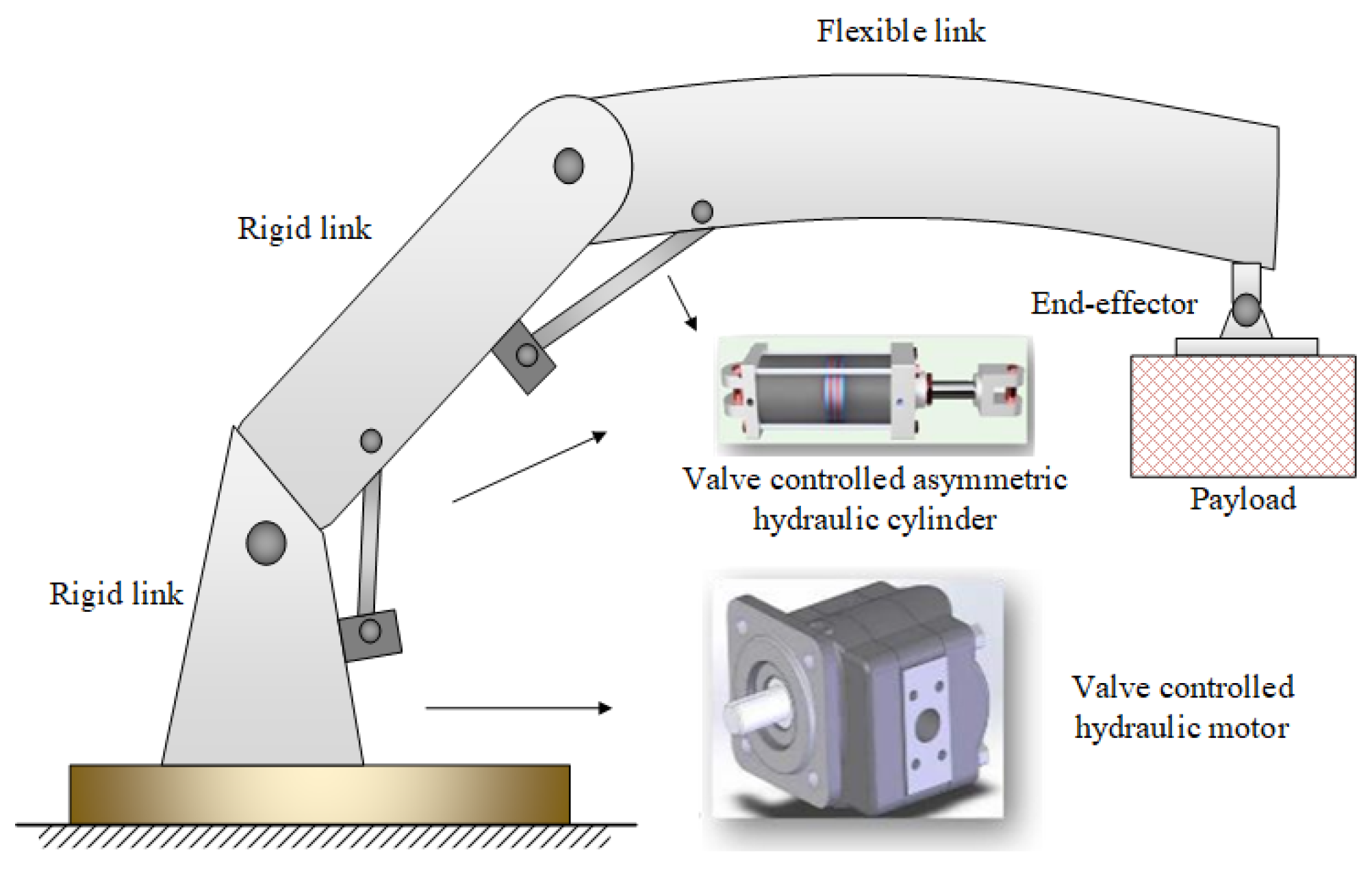
2. Dynamics Modeling of HDFRAs

2.1. Mechanical Subsystem Dynamics Modeling

The mechanical system constructed in this study consists of a three-degree-of-freedom (3-DOF) serial mechanism: the first two segments are rigid rotating links, while the terminal segment employs an elastic beam structure with planar bending characteristics (Figure 1). The primary and secondary segments are rigidly connected via revolute joints, and the flexible terminal link is articulated to the secondary segment through a rotational hinge. Since large-range motions of the end-effector under heavy-load conditions readily induce beam vibrations, the model focuses on transverse vibration characteristics while neglecting axial and shear deformation effects. The flexural vibration dynamics are established based on the Euler–Bernoulli beam theory.

The system’s dynamics modeling involves coupled mechanical and hydraulic subsystems. For the mechanical subsystem, a hybrid strategy integrating assumed mode analysis and energy methods is adopted: the Assumed Mode Method (AMM) resolves flexible-body vibration characteristics, while Lagrange equations govern the derivation of system dynamics. The modeling process follows these assumptions (key parameters are listed in

Table 1. Standard symbols and notations for mechanical subsystems.

Symbol	Definition	Symbol	Definition
${\iota }_j$	length of link j	G	payload mass
${\gamma }_j$	angle of joint j	g	gravitational acceleration
$m_j$	mass of the actuator j	$\kappa$	stiffness coefficient
$R_1$	top face radial dimension of link 1	${\theta }_{11},{\theta }_{21}$	positioning of the primary hydraulic cylinder
$R_2$	bottom face radial dimension of link 1	${\theta }_{22},{\theta }_{31}$	positioning of the secondary hydraulic cylinder
${\varpi }_j$	linear density of link j	${\Gamma }_i\left(R\right)$	$i^{\mathrm{th}}$ oscillation mode characteristic of flexible link 3
$s(l,t)$	elastic deflection of compliant link 3	$p_i\left(t\right)$	$i^{\mathrm{th}}$ oscillatory eigenvector element for flexible link 3

):

Assumption 1.

The end-effector and load are rigidly connected with no relative displacement.

Assumption 2.

Actuator masses are concentrated at joint rotation centers, and the mass distribution of transmission mechanisms is negligible.

To characterize the kinematic properties of the system, an inertial coordinate system YOZ fixed to the base and a moving coordinate system ${\mathrm{Y}}_1{\mathrm{OZ}}_1$ attached to the robotic arm are established. Figure 2 comprehensively illustrates the geometric mapping relationships among four coordinate systems in the HDFRAs. Employing the AMM for modal truncation, the elastic deformation of the compliant structure can be mathematically formulated through modal coordinate synthesis as per Equation (1).

$$s\left(l,t\right)=\sum _{i=1}^n{\Gamma }_i\left(l\right)p_i\left(t\right)$$

(1)

Following the engineering dominant mode principle, only the low-order modes significantly contributing to the system’s dynamic response are retained, while higher-order modes are neglected due to their minimal energy contribution. Specifically, the boundary conditions of flexible link 3 adhere to the cantilever beam hypothesis: the proximal end is constrained by a revolute joint, while the distal end remains in a free deformation state [24]. Consequently, the elastic displacement of link 3 is formulated as

$$s\left(l,t\right)={\Gamma }_1\left(l\right)p_1\left(t\right)+{\Gamma }_2\left(l\right)p_2\left(t\right)$$

(2)

$${\Gamma }_i\left(l\right)=sinh{\alpha }_{i}l+v_{i}sin{\alpha }_{i}l$$

(3)

where $v_i=sinh{\alpha }_i{t}_3/sin{\alpha }_i{t}_3,{\alpha }_i=\left(i+0.25\right)\pi /t_3,i=1,2$; the value 1 characterizes the geometric location of a selected point on the link 3, and $0\le 1\le {\iota }_3$.

Through hybrid rigid–flexible kinematic analysis, the aggregate dynamic energy of the system can be decomposed into the average kinetic energy of rigid links and the elastic potential energy of the flexible link. The mathematical representation is shown in Equation (4):

$$\begin{array}{cc}\hfill K=& \left({\displaystyle \frac{1}{2}}G{{\iota }_2}^2+{\displaystyle \frac{1}{2}}{m}_3{{\iota }_2}^2+{\displaystyle \frac{1}{2}}{\varpi }_3{\iota }_3{{\iota }_2}^2+{\displaystyle \frac{1}{6}}{\varpi }_2{{\iota }_2}^3\right)({\dot{\gamma }}_2^2+{\dot{\gamma }}_1^2{sin}^2{\gamma }_2)\hfill \\ \hfill & +{\dot{\gamma }}_1^2\left[{\displaystyle \frac{1}{2}}{m}_2{R}_1^2+{\displaystyle \frac{1}{6}}{\varpi }_1(R_2^3-R_1^3)\right]+{\varpi }_3{\iota }_2{\int }_0^{{\iota }_3}\dot{s}dl+{\dot{\gamma }}_{2}cos{\gamma }_3\hfill \\ \hfill & +{\displaystyle \frac{1}{2}}G{{\iota }_3}^2\left[{\dot{\gamma }}_1^2{sin}^2({\gamma }_2+{\gamma }_3)+{({\dot{\gamma }}_2+{\dot{\gamma }}_3)}^2\right]+{\displaystyle \frac{1}{2}}{\varpi }_3{\int }_0^{{\iota }_3}{\dot{s}}^{2}dl\hfill \\ \hfill & +\left({\displaystyle \frac{1}{2}}{\varpi }_3{\iota }_2{{\iota }_3}^2+G{\iota }_2{\iota }_3\right)\left[{\dot{\gamma }}_2({\dot{\gamma }}_2+{\dot{\gamma }}_3)cos{\gamma }_3+{\dot{\gamma }}_1^{2}sin{\gamma }_{2}sin({\gamma }_2+{\gamma }_3)\right]\hfill \\ \hfill & +\left({\displaystyle \frac{1}{2}}{\varpi }_3{\int }_0^{{\iota }_3}{s}^{2}dl+{\displaystyle \frac{1}{2}}G{s}_{{\iota }_3}^2\right)\left[{\left({\dot{\gamma }}_2+{\dot{\gamma }}_3\right)}^2+{\dot{\gamma }}_1^2{cos}^2({\gamma }_2+{\gamma }_3)\right]\hfill \\ \hfill & +{\iota }_2\left({\varpi }_3{\int }_0^{{\iota }_3}sdl+G{s}_{{\iota }_3}\right)\left[{\dot{\gamma }}_1^{2}sin{\gamma }_{2}cos({\gamma }_2+{\gamma }_3)-{\dot{\gamma }}_2({\dot{\gamma }}_2+{\dot{\gamma }}_3)sin{\gamma }_3\right]\hfill \\ \hfill & +\left({\varpi }_3{\int }_0^{{\iota }_3}\dot{s}dl+G{\iota }_3{\dot{s}}_{{\iota }_3}\right)\left({\dot{\gamma }}_2+{\dot{\gamma }}_3\right)\hfill \\ \hfill & +\left({\varpi }_3{\int }_0^{{\iota }_3}sdl+G{\iota }_3{s}_{{\iota }_3}\right){\dot{\gamma }}_1^{2}sin({\gamma }_2+{\gamma }_3)cos({\gamma }_2+{\gamma }_3)\hfill \\ \hfill & +{\displaystyle \frac{1}{2}}G{\dot{s}}_{{\iota }_3}^2+G{\iota }_2{\dot{s}}_{{\iota }_3}{\dot{\gamma }}_{2}cos{\gamma }_3+{\displaystyle \frac{1}{6}}{\varpi }_3{{\iota }_3}^3\left[{\left({\dot{\gamma }}_2+{\dot{\gamma }}_3\right)}^2+{\dot{\gamma }}_1^2{sin}^2({\gamma }_2+{\gamma }_3)\right]\hfill \end{array}$$

(4)

The potential energy function of the system consists of three parts: the bending strain energy of the beam, the gravitational potential energy of the joints, and the load potential energy. The specific expression is given in Equation (5):

$$\begin{array}{cc}\hfill U=& g{\iota }_1\left(m_2+m_3+G+{\displaystyle \frac{1}{2}}{\varpi }_1{\iota }_1+{\varpi }_2{\iota }_2+{\varpi }_3{\iota }_3\right)+g{\iota }_{2}cos{\gamma }_2\left(m_3+G+{\displaystyle \frac{1}{2}}{\varpi }_2{\iota }_2+{\varpi }_3{\iota }_3\right)\hfill \\ \hfill & +\left(Gg{\iota }_3+{\displaystyle \frac{1}{2}}{\varpi }_{3}g{{\iota }_3}^2-{\varpi }_{3}g{\int }_0^{{\iota }_3}sdl\right)cos({\gamma }_2+{\gamma }_3)-Gg{s}_{{\iota }_3}sin({\gamma }_2+{\gamma }_3)+{\displaystyle \frac{1}{2}}\kappa {\int }_0^{{\iota }_3}{\left({\displaystyle \frac{{\partial }^{2}s}{\partial l^2}}\right)}^{2}dl\hfill \end{array}$$

(5)

where $s=s(l,t),\dot{s}={\Gamma }_1\left(l\right){\dot{p}}_1\left(t\right)+{\Gamma }_2\left(l\right){\dot{p}}_2\left(t\right),s_{{\iota }_3}={\Gamma }_1\left({\iota }_3\right)p_1\left(t\right)+{\Gamma }_2\left({\iota }_3\right)p_2\left(t\right),{\dot{s}}_{{\iota }_3}={\Gamma }_1\left({\iota }_3\right){\dot{p}}_1\left(t\right)+{\Gamma }_2\left({\iota }_3\right){\dot{p}}_2\left(t\right)$ and ${\displaystyle \frac{{\partial }^{2}s}{\partial l^2}}={\ddot{\Gamma }}_1\left(l\right)p_1\left(t\right)+{\ddot{\Gamma }}_2\left(l\right)p_2\left(t\right)$.

The Lagrange function is defined as $L=K-U$. Based on Lagrange’s equations of the second kind [25]:

$${\displaystyle \frac{{\partial }^{2}s}{\partial l^2}}={\ddot{\Gamma }}_1\left(l\right)p_1\left(t\right)+{\ddot{\Gamma }}_2\left(l\right)p_2\left(t\right)$$

(6)

Under idealized conditions neglecting viscous damping and external disturbances, the coupled dynamics equations of the flexible–rigid system are derived as Equation (7):

$$D(\gamma ,p)\left[\begin{array}{c}\ddot{\gamma }\\ \ddot{p}\end{array}\right]+\Lambda \left[\begin{array}{c}\gamma \\ p\end{array}\right]+\Phi (\gamma ,\dot{\gamma },p,\dot{p})=\left[\begin{array}{c}u\\ 0\end{array}\right]$$

(7)

where $D(\gamma ,p)$ is the $5\times 5$ positive definite matrix; $\Lambda =diag({\kappa }_1,{\kappa }_2)$ is the stiffness matrix of the flexible link 3; $\Phi (\gamma ,\dot{\gamma },p,\dot{p})={\left[g_1{g}_2{g}_3{g}_4{g}_5\right]}^T$, encompassing Coriolis forces, centrifugal forces, and gravitational effects; $\gamma ={\left[{\gamma }_1{\gamma }_2{\gamma }_3\right]}^T$ denotes the joint angles; $p={\left[p_1{p}_2\right]}^T$ denotes the modal coordinates; and $u={\left[u_1{u}_2{u}_3\right]}^T$ denotes the control torques.

Remark 1.

The q in Equation (6) includes joint angles and elastic displacements. When $j=1,2,3$, the system considers joint angles and control torques.

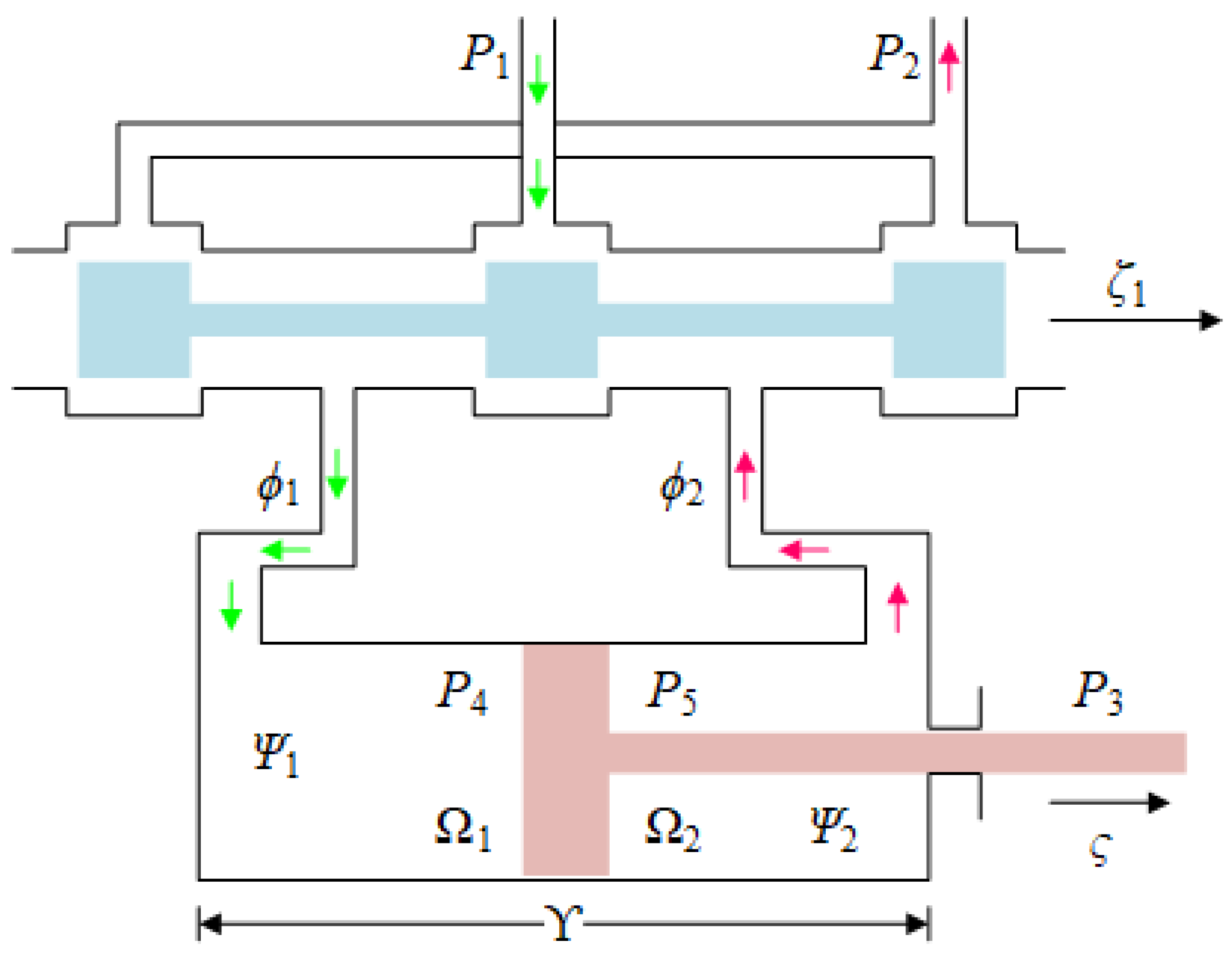
2.2. Hydraulic Subsystem Modeling

The system adopts a hybrid actuation architecture: three distinct actuator types are integrated—a rotary hydraulic motor enabling rotational freedom at Joint 1, while two valve-regulated hydraulic cylinders provide linear actuation for Joints 2 and 3, respectively. As shown in Figure 3, the hydraulic actuation unit integrates two types of actuators: valve-controlled hydraulic cylinders and hydraulic motors, with its parameter system provided in

Table 2. Standard symbols and notations for hydraulic subsystem.

Symbol	Definition	Symbol	Definition
$P_1$	supply pressure	$\upsilon$	equivalent volume
$P_2$	return pressure	$\omega$	flow/pressure coefficient
$P_3$	payload pressure	$\tau$	equivalent leakage coefficient
$P_4,P_5$	L/R chamber pressures of the actuator	${\Omega }_1,{\Omega }_2$	effective working areas of piston chambers
${\varphi }_2,{\varphi }_3$	real-time flow rates in dual-acting cylinder chambers	${\psi }_1,{\psi }_2$	left and right hydraulic chamber effective displacement volume
$V_h$	geometric pumping of the motor	${\sigma }_1$	hydraulic throughput amplification factor
$\phi$	hydraulic orifice flow coefficient	${\varphi }_1$	volumetric flow rate to actuator
$g_a$	area gradient of the valve	${\zeta }_1$	valve core travel distance
$I_s$	electro-hydraulic control signal	$\varsigma$	actuator rod movement range
$\vartheta$	bulk modulus	${\rm Y}$	maximum piston displacement

. The four-way sliding valve-controlled asymmetric hydraulic cylinder converts hydraulic energy to mechanical energy through chamber pressure coupling effects.

Considering the electromechanical timescale separation characteristic (where the mechanical system inertia is significantly larger than the hydraulic valve dynamic response), the servo valve spool displacement ${\zeta }_1$ is linearly related to the control current $I_e$, and its transfer characteristic can be expressed as

$${\zeta }_1=G_e{I}_e$$

(8)

where $G_e=G_v{G}_a$; $G_v$ is the proportional valve gain; and $G_a$ is the amplifier gain.

Based on the mounting positions of the hydraulic cylinders, we can derive

$$\begin{array}{cc}\hfill {\varsigma }_2& =\sqrt{{\theta }_{21}^2+{\theta }_{11}^2-2{\theta }_{11}{\theta }_{21}cos({180}^{\circ }-{\gamma }_2)}\hfill \\ \hfill {\varsigma }_3& =\sqrt{{\theta }_{22}^2+{\theta }_{31}^2-2{\theta }_{22}{\theta }_{31}cos({180}^{\circ }-{\gamma }_3)}\hfill \\ \hfill \dot{\varsigma }& =J\dot{\gamma }\hfill \end{array}$$

(9)

where $J=diag(J_1,J_2)$ denotes the kinematic transformation matrix that converts hydraulic cylinder displacements to joint rotations. The parametric representation takes the form

$$\begin{array}{cc}\hfill J_2& ={\displaystyle \frac{\partial {\varsigma }_2}{\partial {\gamma }_2}}={\displaystyle \frac{-{\theta }_{21}{\theta }_{11}sin{\gamma }_2}{\sqrt{{\theta }_{21}^2+{\theta }_{11}^2+2{\theta }_{11}{\theta }_{21}cos{\gamma }_2}}}\hfill \\ \hfill J_3& ={\displaystyle \frac{\partial {\varsigma }_3}{\partial {\gamma }_3}}={\displaystyle \frac{-{\theta }_{22}{\theta }_{31}sin{\gamma }_3}{\sqrt{{\theta }_{22}^2+{\theta }_{31}^2+2{\theta }_{22}{\theta }_{31}cos{\gamma }_3}}}\hfill \end{array}$$

(10)

Based on the fluid continuity equations and Newtonian dynamics laws [26], the pressure–flow rate equations for the valve-controlled hydraulic cylinder are established:

$$\left\{\begin{array}{cc}\hfill {\zeta }_1& =G_e{I}_s\hfill \\ \hfill u& ={\Omega }_{p}J{P}_3\hfill \\ \hfill {\varphi }_1& ={\sigma }_1{\zeta }_1-\omega P_3\hfill \\ \hfill {\varphi }_1& =\tau P_3+{\displaystyle \frac{\upsilon }{4{\Delta }_p}}{\dot{P}}_3+{\Omega }_p{\dot{\varsigma }}_1\hfill \end{array}\right.,{\Omega }_p=\left\{\begin{array}{ccc}{\Omega }_1,\hfill & \hfill & {\zeta }_1\ge 0\hfill \\ {\Omega }_2,\hfill & \hfill & {\zeta }_1<0\hfill \end{array}\right.$$

(11)

where ${\sigma }_1=\phi g_a\sqrt{(P_1-P_3)/\varpi }$, $\upsilon =2{\rm Y}{{\Omega }_p}^4/({{\Omega }_1}^3+{{\Omega }_2}^3)$.

Combining Equations (9) and (11), we can derive

$$\dot{u}+\left[{\displaystyle \frac{4\vartheta }{\upsilon }}(\omega +\tau )-{\displaystyle \frac{\dot{J}}{J}}\right]u+{\displaystyle \frac{4\vartheta {\Omega }_p^2}{\upsilon }}{J}^2\dot{\gamma }={\displaystyle \frac{4\vartheta {\Omega }_p{\sigma }_1{G}_e}{\upsilon }}J{I}_s$$

(12)

The torque generation mechanism of the valve-controlled hydraulic motor is described by the equivalent chamber model in Equation (13). Through a simplified derivation of Equation (13), the current-to-torque transfer function (Equation (14)) can be obtained:

$$\left\{\begin{array}{cc}\hfill {\zeta }_1& =G_e{I}_s\hfill \\ \hfill u& =P_3{V}_h\hfill \\ \hfill {\varphi }_1& ={\sigma }_1{\zeta }_1-\omega P_3\hfill \\ \hfill {\varphi }_1& =\tau P_3+{\displaystyle \frac{\upsilon }{4\vartheta }}{\dot{P}}_3+V_h\dot{\gamma }\hfill \end{array}\right.$$

(13)

$$\dot{u}+{\displaystyle \frac{4\vartheta }{\upsilon }}(\omega +\tau )u+{\displaystyle \frac{4\vartheta V_h^2}{\upsilon }}\dot{\gamma }={\displaystyle \frac{4\vartheta V_h{\sigma }_1{G}_e}{\upsilon }}{I}_s$$

(14)

For clarity of presentation, Equation (14) is reformulated as Equation (15):

$$\dot{u}+Au+B\dot{\gamma }=C{I}_s$$

(15)

where $A={\displaystyle \frac{4\vartheta }{\upsilon }}(\omega +\tau ),B={\displaystyle \frac{4\vartheta V_h^2}{\upsilon }},C={\displaystyle \frac{4\vartheta V_h{\sigma }_1{G}_e}{\upsilon }}$.

The hydraulic subsystem model Equation (15) and the mechanical subsystem model Equation (7) together form the dynamic model of HDFRAs, revealing the system’s inherent strong nonlinear coupling characteristics. Specifically,

$$\left\{\begin{array}{c}D(\gamma ,p)\left[\begin{array}{c}\ddot{\gamma }\\ \ddot{p}\end{array}\right]+\Lambda \left[\begin{array}{c}\gamma \\ p\end{array}\right]+\Phi (\gamma ,\dot{\gamma },p,\dot{p})=\left[\begin{array}{c}u\\ 0\end{array}\right]\hfill \\ \dot{u}+Au+B\dot{\gamma }=C{I}_s\hfill \end{array}\right.$$

(16)

3. The Singular Perturbation Decoupling of HDFRA System

The governing equations of HDFRAs constitute a strongly nonlinear differential system with time-dependent high-order dynamics, where its multi-physics coupling characteristics pose challenges, including lack of decoupling conditions and sensitivity to parameter perturbations for controller design. This section establishes a dual-scale decomposition framework based on SPT, performs two-stage decoupling on the original system, and decouples it into a second-order rigid-body motion subsystem (SRS), a second-order flexible vibration subsystem (SFS), and a first-order hydraulic dynamic subsystem (FHS), achieving layered control of HDFRAs’ coupled dynamics.

3.1. First-Order Singular Perturbation Decoupling

Define the first perturbation parameter ${\delta }_1=1/g$, satisfying $0<{\delta }_1\ll 1$, and reformulate the complete dynamic Equation (16) into the perturbed form shown in Equation (17):

$$\left\{\begin{array}{c}D(\gamma ,p)\left[\begin{array}{c}\ddot{\gamma }\\ \ddot{p}\end{array}\right]+\Lambda \left[\begin{array}{c}\gamma \\ p\end{array}\right]+\Phi (\gamma ,\dot{\gamma },p,\dot{p})=\left[\begin{array}{c}u\\ 0\end{array}\right]\hfill \\ {\delta }_1\dot{u}=-\tilde{A}u-\tilde{B}\dot{\gamma }+\tilde{C}{I}_s\hfill \end{array}\right.$$

(17)

where $\tilde{A}={\delta }_{1}A$, $\tilde{B}={\delta }_{1}B$, $\tilde{C}={\delta }_{1}C$.

When ${\delta }_1$ approaches zero, higher-order infinitesimal terms can be neglected. According to multi-timescale theory, the control torque u and control input $I_s$ can be decomposed into fast and slow components:

$$\begin{array}{cc}\hfill u& =u_{a1}+u_{b1}\hfill \\ \hfill I_s& =I_{a1}+I_{b1}\hfill \end{array}$$

(18)

where the subscripts $a1$ and $b1$ represent the fast and slow timescale components, respectively. By setting ${\delta }_1=0$, the first-order slow subsystem (FSS) can be obtained as shown in Equation (19):

$$\left\{\begin{array}{c}\mathrm{D}(\gamma ,p)\left[\begin{array}{c}\ddot{\gamma }\\ \ddot{p}\end{array}\right]+\Lambda \left[\begin{array}{c}\gamma \\ p\end{array}\right]+\Phi (\gamma ,\dot{\gamma },p,\dot{p})=\left[\begin{array}{c}{u}_{b1}\\ 0\end{array}\right]\hfill \\ u_{b1}=-{\tilde{A}}^{-1}\tilde{B}\dot{\gamma }+{\tilde{A}}^{-1}\tilde{C}{I}_{b1}\hfill \end{array}\right.$$

(19)

Introducing the fast timescale defined in Equation (20), $u_{b1}$ is treated as a constant within the neighborhood of ${\delta }_1\to 0$. By combining Equations (17) and (19), the FHS can be derived as Equation (21):

$${\rho }_1={\displaystyle \frac{t}{{\delta }_1}}$$

(20)

$${\displaystyle \frac{d{u}_{a1}}{d{\rho }_1}}=-\tilde{A}{u}_{a1}+\tilde{C}{I}_{a1}$$

(21)

3.2. Second-Order Singular Perturbation Decoupling

To perform a second decoupling of the FSS, we separate the slow rigid-body motion subsystem (SRS) and the slow flexible vibration subsystem (SFS). Define the inverse matrix of $\mathrm{G}$ as $\mathrm{N}$, as shown in Equation (22):

$$N=G^{-1}=\left[\begin{array}{cc}{G}_1& G_2\\ G_3& G_4\end{array}\right]=\left[\begin{array}{cc}{N}_1& N_2\\ N_3& N_4\end{array}\right]$$

(22)

where $G_1\in {\mathbb{R}}^{3\times 3}$, $N_1\in {\mathbb{R}}^{3\times 3}$.

The generalized force vector is constructed as given in Equation (23):

$$\Phi (\gamma ,\dot{\gamma },p,\dot{p})=\left[\begin{array}{c}{\Phi }_1\\ {\Phi }_2\end{array}\right]$$

(23)

By combining Equations (19), (22) and (23), we obtain

$$\begin{array}{cc}\hfill \ddot{\gamma }& =-N_2(\gamma ,p){\Xi }_{x}p-N_1(\gamma ,p){\Phi }_1(\gamma ,\dot{\gamma },p,\dot{p})\hfill \\ \hfill & -N_2(\gamma ,p){\Phi }_2(\gamma ,\dot{\gamma },p,\dot{p})+N_1(\gamma ,p)\left(-{\tilde{A}}^{-1}\tilde{B}\dot{\gamma }+{\tilde{A}}^{-1}\tilde{C}{I}_{b1}\right)\hfill \end{array}$$

(24)

$$\begin{array}{cc}\hfill \ddot{p}& =-N_4(\gamma ,p){\Xi }_{x}p-N_3(\gamma ,p){\Phi }_1(\gamma ,\dot{\gamma },p,\dot{p})\hfill \\ \hfill & -N_4(\gamma ,p){\Phi }_2(\gamma ,\dot{\gamma },p,\dot{p})+N_3(\gamma ,p)\left(-{\tilde{A}}^{-1}\tilde{B}\dot{\gamma }+{\tilde{A}}^{-1}\tilde{C}{I}_{b1}\right)\hfill \end{array}$$

(25)

where ${\Xi }_x=\left[\begin{array}{c}{\Xi }_1\\ {\Xi }_2\end{array}\right]$.

Define the second perturbation parameter ${\delta }_2=1{/}_{\Xi }$, where $\Xi =min({\Xi }_1,{\Xi }_2)$, $0<{\delta }_1\ll {\delta }_2\ll 1$.

Similarly, based on multi-timescale theory and neglecting higher-order terms $o\left({\delta }_2\right)$, variables $\varsigma$ and $I_{b1}$ can be decomposed into second-order fast and slow components:

$$\left\{\begin{array}{c}\varsigma ={\varsigma }_{a2}+{\varsigma }_{b2}\hfill \\ I_{b1}=I_{a2}+I_{b2}\hfill \end{array}\right.$$

(26)

where the subscripts $a2$ and $b2$ represent the fast and slow timescales of the second stage, respectively.

Through variable substitution in Equation (27) and setting ${\delta }_2=0$, combined with Equations (24), (25) and (27), we can derive Equations (28) and (29):

$$\left\{\begin{array}{c}\tilde{\Xi }={\delta }_2{\Xi }_x\hfill \\ p={\delta }_2\varsigma \hfill \end{array}\right.$$

(27)

$$\begin{array}{cc}\hfill \ddot{\gamma }=& -N_{2,b2}(\gamma ,0)\tilde{\Xi }{\varsigma }_{b2}-N_{1,b2}(\gamma ,0){\Phi }_{1,b2}(\gamma ,\dot{\gamma },0,0)\hfill \\ \hfill & -N_{2,s2}(\gamma ,0){\Phi }_{2,b2}(\gamma ,\dot{\gamma },0,0)+N_{1,b2}(\gamma ,0)\left(-{\tilde{A}}^{-1}\tilde{B}\dot{\gamma }+{\tilde{A}}^{-1}\tilde{C}{I}_{b2}\right)\hfill \end{array}$$

(28)

$$\begin{array}{cc}\hfill 0=& -N_{4,b2}(\gamma ,0)\tilde{\Xi }{\varsigma }_{b2}-N_{3,b2}(\gamma ,0){\Phi }_{1,b2}(\gamma ,\dot{\gamma },0,0)\hfill \\ \hfill & -N_{4,b2}(\gamma ,0){\Phi }_{2,b2}(\gamma ,\dot{\gamma },0,0)+N_{3,b2}(\gamma ,0)\left(-{\tilde{A}}^{-1}\tilde{B}\dot{\gamma }+{\tilde{A}}^{-1}\tilde{C}{I}_{b2}\right)\hfill \end{array}$$

(29)

Solving Equation (29) yields ${\varsigma }_{b2}$, as shown in Equation (30). Substituting this back into Equation (28) gives the SRS Equation (31):

$$\begin{array}{cc}\hfill {\varsigma }_{b2}=& -{\tilde{\Xi }}^{-1}{N}_{4,b2}^{-1}(\gamma ,0)N_{3,b2}(\gamma ,0){\Phi }_{1,b2}(\gamma ,\dot{\gamma },0,0)\hfill \\ \hfill & -{\tilde{\Xi }}^{-1}{N}_{4,b2}^{-1}(\gamma ,0)N_{4,b2}(\theta ,0){\Phi }_{2,b2}(\gamma ,\dot{\gamma },0,0)\hfill \\ \hfill & +{\tilde{\Xi }}^{-1}{N}_{4,b2}^{-1}(\gamma ,0)N_{3,b2}(\gamma ,0)\left(-{\tilde{A}}^{-1}\tilde{B}\dot{\gamma }+{\tilde{A}}^{-1}\tilde{C}{I}_{b2}\right)\hfill \end{array}$$

(30)

$$G_{1,b2}(\gamma ,0)\ddot{\gamma }+{\Phi }_{1,b2}(\gamma ,\dot{\gamma },0,0)=-{\tilde{A}}^{-1}\tilde{B}\dot{\gamma }+{\tilde{A}}^{-1}\tilde{C}{I}_{b2}$$

(31)

By introducing the second-order fast timescale Equation (32), ${\varsigma }_{b2}$ is treated as a constant within the neighborhood of ${\delta }_2\to 0$. Combining Equations (25), (26) and (30), the SFS dynamic Equation (33) is ultimately established:

$${\rho }_2={\displaystyle \frac{t}{\sqrt{{\delta }_2}}}$$

(32)

$${\displaystyle \frac{d^2{\varsigma }_{a2}}{d{\rho }_2^2}}=N_{3,b2}(\gamma ,{\delta }_2\varsigma ){\tilde{A}}^{-1}\tilde{C}{I}_{a2}-N_{4,b2}(\gamma ,{\delta }_2\varsigma )\tilde{\Xi }{\varsigma }_{a2}$$

(33)

4. Controller Design

4.1. AFTSM-ADRC Design for Second-Order Systems

The proposed AFTSM-ADRC retains the ADRC framework’s core structure while innovatively substituting its conventional nonlinear feedback mechanism with fast terminal sliding mode dynamics to boost robustness and response speed.

The controller design process begins with deriving the SRS state-space representation. Let $\mathit{x}={\left[{\mathit{x}}_1,{\mathit{x}}_2\right]}^{\mathrm{T}}={\left[\gamma ,\dot{\gamma }\right]}^{\mathrm{T}}$, and considering the uncertainties and disturbances present in a practical system operation, the SRS Equation (30) can be rewritten as

$$\left\{\begin{array}{c}{\dot{x}}_1=x_2\hfill \\ {\dot{x}}_2=f\left(x\right)+g\left(x\right)I_{s2}+d\hfill \end{array}\right.$$

(34)

where $\mathit{f}\left(\mathit{x}\right)=-G_{1,b}^{-1}\left(\gamma ,0\right)\ddot{\gamma }\left[{\Phi }_{1,b2}\left(\gamma ,\dot{\gamma },0,0\right)+{\tilde{A}}^{-1}\tilde{B}\dot{\gamma }\right],\mathit{g}\left(\mathit{x}\right)=G_{1,b2}^{-1}\left(\gamma ,0\right){\tilde{A}}^{-1}\tilde{C},d$ represents the lumped uncertainties and disturbances for the SRS.

Assumption 3.

The lumped uncertainties and disturbances $\mathit{d}$ for the SRS are bounded above by ${\mathit{d}}^{*}$, i.e., $\Vert \mathit{d}\Vert \le {\mathit{d}}^{*}$.

4.1.1. Design of Tracking Differentiator

The nonlinear tracking differentiator employed in this study is expressed as follows:

$$\left\{\begin{array}{c}{x}_1(k+1)=x_1\left(k\right)+T·x_2\left(k\right)\hfill \\ x_2(k+1)=x_2\left(k\right)+T·fst(x_1\left(k\right)-v\left(k\right),x_2\left(k\right),\delta ,T)\hfill \end{array}\right.$$

(35)

where $\mathit{T}$ is the integration step size; $\mathit{v}\left(k\right)$ indicates the k-th sampling instant input; ${\mathit{x}}_1\left(k\right)$ represents the filtered version of $v\left(k\right)$; ${\mathit{x}}_2\left(k\right)$ is the differential signal of $v\left(k\right)$; $\delta$ is a parameter determining tracking speed; and $fst(·)$ specifies the optimal control synthesis operator, defined as

$$fst(x_1,x_2,\delta ,T)=\left\{\begin{array}{cc}-\delta sgn\left(a\right)\hfill & \left|a\right|>r\hfill \\ -\delta {\displaystyle \frac{a}{r}}\hfill & \left|a\right|\le r\hfill \end{array}\right.$$

(36)

$$a=\left\{\begin{array}{cc}{x}_2+{\displaystyle \frac{y}{T}}\hfill & \left|y\right|\le d_0\hfill \\ x_2+{\displaystyle \frac{a_0-r}{2}}sgn\left(y\right)\hfill & \left|y\right|>d_0\hfill \end{array}\right.$$

(37)

where $\mathit{y}={\mathit{x}}_1+T{\mathit{x}}_2$; $\mathit{r}=\delta T$; ${\mathit{d}}_0=T\mathit{r}$; ${\mathit{a}}_0=\sqrt{{\mathit{r}}^2+8\delta \left|\mathit{y}\right|}$; and $sgn(·)$ denotes the sign function. This structure ensures rapid and smooth tracking of input signals while minimizing noise amplification.

4.1.2. Design of the BESO

To estimate the system’s lumped disturbances, it is first necessary to introduce an extended state variable to characterize their dynamic behavior. In this study, the $\mathit{f}\left(\mathit{x}\right)+\mathit{d}$ in the decoupled SRS are expanded into a new state variable, expressed as

$$x_3=f\left(x\right)+d=-G_{1,b2}^{-1}(\gamma ,0)\ddot{\gamma }\left[{\Phi }_{1,b2}(\gamma ,\dot{\gamma },0,0)+{\tilde{A}}^{-1}\tilde{B}\dot{\gamma }\right]+d$$

(38)

According to Equations (34) and (38), the system equation of SRS can be expressed as

$$\left\{\begin{array}{c}{\dot{x}}_1=x_2\hfill \\ {\dot{x}}_2=g\left(x\right)I_{b2}+x_3\hfill \end{array}\right.$$

(39)

In traditional extended state observer (ESO) parameter tuning, larger observer bandwidth is typically selected to accelerate response speed and reduce estimation error. However, this tends to amplify system noise and compromise closed-loop stability. To enhance the observation capability and accuracy of the ESO, inspired by ref. [27], this paper proposes a BESO formulated as follows:

$$\left\{\begin{array}{cc}\hfill \xi & =z_1-x_{2d}\hfill \\ \hfill \gamma & ={\eta }^{-sgn\left({\displaystyle \frac{d\left|\xi \right|}{dt}}\right)}\hfill \\ \hfill {\dot{z}}_1& =g\left(x\right)I_{b2}+z_2+{\beta }_1\theta \xi \hfill \\ \hfill {\dot{z}}_2& ={\beta }_2\theta \xi \hfill \end{array}\right.$$

(40)

where $x_{2d}$ represents the desired value of $x_2$; ${\beta }_1=-2{\omega }_0$, ${\beta }_2=-{\omega }_0^2$, with ${\omega }_0$ being the system bandwidth; $\theta >0$, $\eta >0$; and $z_1$ and $z_2$ denote the observed values of $x_2$ and $X_3$, respectively. Compared to conventional ESOs, the proposed BESO estimates system states based on observation errors and adaptively adjusts gain parameters according to both the magnitude and rate of change of these errors, thereby achieving superior observation performance.

4.1.3. Design of Adaptive Reaching Law

Conventional power-rate convergence dynamics take the form [28]: $\dot{\mathrm{s}}=-\mu {\left|\mathrm{s}\right|}^{{\alpha }_0}sgn\left(\mathrm{s}\right)$ where $\mu >0,0<{\alpha }_0<1$. At the initial stage of system response, the approaching dynamics exhibit accelerated convergence when the error metric s exceeds critical thresholds. However, during the convergence phase $\left(\Vert s\Vert \to 0\right)$, the power-rate reaching law exhibits velocity attenuation, leading to extended settling time and degraded transient performance of the closed-loop system.

The variable-speed reaching law is expressed as [28] $\dot{\mathrm{s}}=-\mu \left|\chi \right|sgn\left(\mathrm{s}\right)$ where $\mu >0$. The sliding mode boundary layer thickness contracts proportionally with $\left|\chi \right|$. Oversized $\mu$ induces persistent chattering upon surface arrival, whereas undersized $\mu$ undesirably restricts the achievable control bandwidth.

For these reasons, this study proposes an adaptive reaching law based on the variable-speed reaching law and power reaching law. Providing dual advantages of robust performance improvement and state-dependent chattering adaptation, the proposed law achieves finite-time sliding surface attainment through its second-order dynamics. Even when the system is subject to bounded external disturbances, it can ensure rapid state convergence and maintain stability at equilibrium. The proposed reaching law is

$$\dot{s}=-k_1{\left|s\right|}^{{\alpha }_0}sgn\left(s\right)-{\epsilon }^{\prime }sgn\left(s\right)-k_3{|\dot{e}|}^{{\beta }_0}·s$$

(41)

where $k_1>0;k_3>0;{\alpha }_0>0;{\beta }_0>0;{\epsilon }^{\prime }=k_2·tanh\left(|\dot{e}|\right);tanh\left(|\dot{e}|\right)=1-{\displaystyle \frac{2}{1+e^{c|\dot{e}|}}}$; $k_2>0;c>0;\dot{e}$ represents the system tracking error; and s denotes the designed sliding surface.

The reaching law shown in Equation (41) consists of three parts: $-k_1{\left|s\right|}^{{\alpha }_0}sgn\left(s\right)$, $-{\epsilon }^{\prime }sgn\left(s\right)$, and $-k_3{|\dot{e}|}^{{\beta }_0}·s$. At the initial stage of system response, when the tracking error is far from the sliding surface, $-k_1{\left|s\right|}^{{\alpha }_0}sgn\left(s\right)$ and $-k_3{|\dot{e}|}^{{\beta }_0}·s$ play dominant roles. Moreover, when $e_1\to \infty$, $lim{\epsilon }^{\prime }=k_2·lim\left[1-{\displaystyle \frac{2}{1+e^{c|\dot{e}|}}}\right]=k_2$, which can further accelerate the system’s reaching speed toward the sliding surface. As the tracking error trajectory approaches the sliding surface, $-k_1{\left|s\right|}^{{\alpha }_0}sgn\left(s\right)$ and $-k_3{|\dot{e}|}^{{\beta }_0}·s$ gradually diminish to zero due to the reduction in s, while $-{\epsilon }^{\prime }sgn\left(s\right)$ becomes dominant. When the system state moves along the sliding surface, ${\epsilon }^{\prime }$ decreases with the reduction in tracking error $\epsilon$, ultimately achieving stability.

4.1.4. Design of AFTSM-ADRC

Define the desired trajectory of SRS as $x_d={\left[x_{1d},x_{2d}\right]}^T={\left[{\gamma }_d,{\dot{\gamma }}_d\right]}^T$, then the error equation of SRS is

$$\left\{\begin{array}{c}e=x_{1\mathrm{d}}-x_1\hfill \\ \dot{e}=x_{2\mathrm{d}}-x_2\hfill \end{array}\right.$$

(42)

Define the fast terminal sliding mode function as

$$s=e+\alpha e^{a/b}+\beta {\dot{e}}^{p/q}$$

(43)

where $\alpha ,\beta >0;a,b,p,q$ are positive odd integers, satisfying $1<p/q<2,a/b>p/q$.

Taking the time derivative of Equation (43) and substituting Equations (39) and (42) yields

$$\dot{s}=\dot{e}+\alpha {\displaystyle \frac{a}{b}}{e}^{a/b-1}\dot{e}+\beta {\displaystyle \frac{p}{q}}{\dot{e}}^{p/q-1}\left({\dot{x}}_{2d}-g\left(x\right)I_{s2}-x_3\right)$$

(44)

Setting the right side of Equation (44) to zero and replacing $x_3$ with its observed value $z_2$, the equivalent control part is obtained:

$$I_{b2eq}={\displaystyle \frac{1}{g\left(x\right)}}\left[{\dot{x}}_{2d}-z_2+{\left(\beta {\displaystyle \frac{p}{q}}\right)}^{-1}{\dot{e}}^{2-p/q}\left(1+\alpha {\displaystyle \frac{a}{b}}{e}^{a/b-1}\right)\right]$$

(45)

Additionally, based on the designed reaching law (41), the switching control part is derived as follows:

$$I_{b2sw}={\displaystyle \frac{1}{g\left(x\right)}}\left[k_1{\left|s\right|}^{{\alpha }_0}sgn\left(s\right)+{\epsilon }^{\prime }sgn\left(s\right)+k_3{\left|\dot{e}\right|}^{{\beta }_0}s\right]$$

(46)

According to sliding mode control theory, the control law of the proposed AFTSM-ADRC is

$$\begin{array}{cc}\hfill I_{b2}& =I_{b2eq}+I_{b2sw}\hfill \\ \hfill & ={\displaystyle \frac{1}{g\left(x\right)}}\left[{\dot{x}}_{2d}-z_2+{\left(\beta {\displaystyle \frac{p}{q}}\right)}^{-1}{\dot{e}}^{2-p/q}\left(1+\alpha {\displaystyle \frac{a}{b}}{e}^{a/b-1}\right)\right.\hfill \\ \hfill & \left.+k_1{\left|s\right|}^{{\alpha }_0}sgn\left(s\right)+{\epsilon }^{\prime }sgn\left(s\right)+k_3{\left|\dot{e}\right|}^{{\beta }_0}s\right]\hfill \end{array}$$

(47)

Theorem 1.

For the system shown in Equation (34), under the conditions satisfying Assumption 3, if the nonlinear tracking differentiator is designed as Equation (35), the system’s BESO is designed as Equation (40), and the control law is designed as Equation (47), then the controlled system (34) is finite-time stable, and the sliding variable s can converge to a finite neighborhood in finite time, i.e., $\left|s\right|\le {\left({\displaystyle \frac{{\tilde{z}}_{max}}{k_1}}\right)}^{1/{\alpha }_0}$

Proof. 

According to Lyapunov stability theory, design the Lyapunov function as

$$V={\displaystyle \frac{1}{2}}{s}^2$$

(48)

Substituting Equation (44) into the time derivative of Equation (47) yields

$$\dot{V}=s\dot{s}=s\left[\dot{e}+\alpha {\displaystyle \frac{a}{b}}{e}^{a/b-1}\dot{e}+\beta {\displaystyle \frac{p}{q}}{\dot{e}}^{p/q-1}\left({\dot{x}}_{2d}-g\left(x\right)I_{s2}-x_3\right)\right]$$

(49)

Define the observation error of BESO for the lumped disturbance $x_3$ as $\tilde{z}$, then

$$\tilde{z}=z_2-x_3$$

(50)

Substituting Equations (47) and (50) into Equation (49) and then simplifying gives

$$\begin{array}{cc}\hfill \dot{V}& =s\left[\dot{e}+\alpha {\displaystyle \frac{a}{b}}{e}^{a/b-1}\dot{e}+\beta {\displaystyle \frac{p}{q}}{\dot{e}}^{p/q-1}\left(-{\left(\beta {\displaystyle \frac{p}{q}}\right)}^{-1}{\dot{e}}^{2-p/q}\left(1+\alpha {\displaystyle \frac{a}{b}}{e}^{a/b-1}\right)\right.\right.\hfill \\ \hfill & \left.\left.-k_1{\left|s\right|}^{{\alpha }_0}sgn\left(s\right)-{\epsilon }^{\prime }sgn\left(s\right)-k_3{\left|\dot{e}\right|}^{{\beta }_0}+\tilde{z}\right)\right]\hfill \\ \hfill & =\beta {\displaystyle \frac{p}{q}}{\dot{e}}^{p/q-1}\left[-k_1{\left|s\right|}^{{\alpha }_0+1}-{\epsilon }^{\prime }\left|s\right|-k_3{\left|\dot{e}\right|}^{{\beta }_0}·s^2+\tilde{z}·s\right]\hfill \\ \hfill & \le \beta {\displaystyle \frac{p}{q}}{\dot{e}}^{p/q-1}\left[-k_1{\left|s\right|}^{{\alpha }_0+1}-{\epsilon }^{\prime }\left|s\right|-k_3|\dot{e}{|}^{{\beta }_0}·s^2+|\tilde{z}|·|s|\right]\hfill \\ \hfill & \le -\beta {\displaystyle \frac{p}{q}}{\dot{e}}^{p/q-1}\left[\left(k_1{\left|s\right|}^{{\alpha }_0}-\left|\tilde{z}\right|\right)\left|s\right|+{\epsilon }^{\prime }\left|s\right|+k_3{\left|\dot{e}\right|}^{{\beta }_0}{s}^2\right]\hfill \end{array}$$

(51)

In Equation (51), as long as appropriate parameters are selected such that $k_3\ge 0$, ${\epsilon }^{\prime }\ge 0$, and $k_i{\left|s\right|}^{{\alpha }_0}\ge {\tilde{z}}_{max}$, then $\dot{V}\le 0$, and the system achieves finite-time convergence to the neighborhood as follows:

$$\left|s\right|\le {\left({\displaystyle \frac{{\tilde{z}}_{max}}{k_1}}\right)}^{1/{\alpha }_0}$$

(52)

The finite-time convergence characteristics of the system will be further demonstrated below.

By applying Young’s inequality [29], Equation (51) can be further expanded as

$$\dot{V}\le -\beta {\displaystyle \frac{p}{q}}{\dot{e}}^{p/q-1}\left[k_1{\left|s\right|}^{{\alpha }_0+1}+{\epsilon }^{\prime }\left|s\right|+k_3{\left|\dot{e}\right|}^{{\beta }_0}{s}^2\right]$$

(53)

When the system trajectory deviates significantly from the sliding surface, Equation (52) can be rewritten as

$$\dot{V}⩽-\beta {\displaystyle \frac{p}{q}}{\dot{e}}^{p/q-1}{k}_1|s{|}^{{\alpha }_0+1}$$

(54)

Substituting Equation (48) into Equation (53) yields

$$\dot{V}⩽-k_1^{\prime }\beta {\displaystyle \frac{p}{q}}{\dot{e}}^{p/q-1}{V}^{\left({\alpha }_0+1\right)/2}$$

(55)

where $k_1^{\prime }=2^{({\alpha }_0+1)/2}{k}_1$.

According to the finite-time stability Lemma [30], the system will converge within a finite time $T\le {\displaystyle \frac{V{\left(0\right)}^{1-({\alpha }_0+1)/2}}{k_1^{\prime }{\beta }_q^p{\dot{e}}^{p/q-1}\left(1-\left({\alpha }_0+1\right)/2\right)}}$, when the exponents satisfy ${\displaystyle \frac{{\alpha }_0+1}{2}}\in (0,1)$, i.e., ${\alpha }_0\in (0,1)$. In the controller parameter design, we impose the constraint ${\alpha }_0\in (0,1)$, ensuring ${\dot{e}}^{p/q-1}>0$ holds consistently, thereby satisfying the finite-time convergence conditions. □

Observation of SFS (33) and SRS (29): It can be observed that the expressions of these two subsystems are similar. Therefore, the SFS can adopt the same controller design as the SRS.

Let $y={\left[y_1,y_2\right]}^T={\left[{\zeta }_{a2},{\displaystyle \frac{d{\zeta }_{a2}}{d{\rho }_2}}\right]}^T$, then the SFS (33) can be rewritten as

$$\left\{\begin{array}{c}{\dot{y}}_1=y_2\hfill \\ {\dot{y}}_2=f\left(y\right)+g\left(y\right)I_{a2}\hfill \end{array}\right.$$

(56)

where $f\left(y\right)=-N_{4,b2}(\gamma ,\_2\varsigma )\tilde{\Xi }{y}_1$, $g\left(y\right)=N_{3,b2}(\gamma ,\_2\varsigma ){\tilde{A}}^{-1}\tilde{C}$.

Following the form of Equation (47), the control law for SFS (56) is derived as

$$I_{a2}={\displaystyle \frac{1}{g\left(y\right)}}\left[{\dot{y}}_{2d}-z_2+{\left(\beta {\displaystyle \frac{p}{q}}\right)}^{-1}{\dot{e}}^{2-p/q}\left(1+\alpha {\displaystyle \frac{a}{b}}{e}^{a/b-1}\right)+k_1{\left|s\right|}^{{\alpha }_0}sgn\left(s\right)+{\epsilon }^{\prime }sgn\left(s\right)+k_3{\left|e_1\right|}^{{\beta }_0}s\right]$$

(57)

4.2. SMO-ISMCC Design for First-Order Systems

In practical applications, hydraulic servo control systems inevitably contain unmodeled uncertainties, including parameter variations of modeled systems, external disturbances, actuator nonlinearities, and load changes. Therefore, the FHS considering uncertainties can be expressed as

$${\displaystyle \frac{d{u}_{a1}}{d{\rho }_1}}=-{\tilde{A}}_0{u}_{a1}+{\tilde{C}}_0{I}_{a1}+d_1$$

(58)

where $d_1=\Delta \tilde{A}{u}_{a1}-\Delta \tilde{C}{I}_{a1}$ represents the lumped uncertainty of FHS.

Assumption 4.

The lumped uncertainty $d_1$ of FHS and its first-order derivative ${\dot{d}}_1$ are bounded, i.e., $|d_1|\le D_1,\left|{\dot{d}}_1\right|\le D_2$.

4.2.1. Design of Sliding Mode Observer

To address the issues of model uncertainties and disturbances in system (58), it is necessary to develop a composite control strategy incorporating a sliding mode observer to achieve high-precision tracking and disturbance rejection capabilities. The sliding mode observer is designed as follows:

$$\left\{\begin{array}{c}{\dot{\widehat{u}}}_{a1}=-{\tilde{A}}_0{\widehat{u}}_{a1}+{\tilde{C}}_0{I}_{a1}+{\widehat{d}}_1+\lambda sat\left({\displaystyle \frac{e_2}{{ϵ}_1}}\right)\hfill \\ {\dot{\widehat{d}}}_1={\lambda }_3{e}_2\hfill \end{array}\right.$$

(59)

where $\lambda$ and ${\lambda }_3$ are observer gains; ${ϵ}_1$ is the boundary layer thickness; and ${\widehat{d}}_1$ and ${\widehat{u}}_{a1}$ are the observed values of $d_1$ and $u_{a1}$, respectively. The saturation operator $sat\left(X\right)$ takes the following form:

$$sat\left(X\right)=\left\{\begin{array}{cc}sgn\left(X\right)\hfill & ,X\ge 1\hfill \\ X\hfill & ,X<1\hfill \end{array}\right.$$

(60)

4.2.2. Design of Integral Sliding Mode Controller

Precision tracking performance necessitates meticulous controller synthesis. First, define the tracking error $e_1$, observation error $e_2$, and disturbance error ${\tilde{d}}_1$ as

$$\left\{\begin{array}{c}{e}_1=u_{a1ref}-u_{a1}\hfill \\ e_2=u_{a1}-{\widehat{u}}_{a1}\hfill \\ {\tilde{d}}_1=d_1-{\widehat{d}}_1\hfill \end{array}\right.$$

(61)

Then, to eliminate steady-state error, an integral term is introduced, and the sliding surface $s_1$ is designed as

$$s_1=e_1+{\lambda }_1{\int }_0^{{\rho }_1}{e}_{1}dt$$

(62)

where ${\lambda }_1>0$ is the integral gain that determines the error convergence rate.

Substituting the system model (58) into the time derivative of the sliding surface (62) yields

$${\dot{s}}_1={\dot{e}}_1+{\lambda }_1{e}_1={\dot{u}}_{a1ref}+{\tilde{A}}_b{u}_{a1}-{\tilde{C}}_0{I}_{a1}-d_1+{\lambda }_1{e}_1$$

(63)

Let ${\dot{s}}_1=-{\lambda }_{2}sat(s_1/{ϵ}_2)$, and substitute the observed values from the observer (59) to obtain the sliding mode control law:

$$I_{a1}={\displaystyle \frac{1}{{\tilde{C}}_0}}\left[{\dot{u}}_{a1\mathrm{ref}}+{\tilde{A}}_b{u}_{a1}+{\lambda }_1{e}_1+{\lambda }_{2}sat(s_1/{ϵ}_2)-{\widehat{d}}_1\right]$$

(64)

where ${\lambda }_2>D_1$ is the sliding mode gain, and ${ϵ}_2$ is the boundary layer thickness.

Theorem 2.

For the system shown in Equation (58), under the conditions satisfying Assumption 4, if the sliding mode observer is designed as Equation (59) and the control law is designed as Equation (64), then the controlled system Equation (58) is input-to-state stable (ISS), and all errors are ultimately bounded.

Proof. 

According to the Lyapunov stability theory, design the Lyapunov function as

$$V_1={\displaystyle \frac{1}{2}}{s}_1^2+{\displaystyle \frac{1}{2}}{e}_2^2+{\displaystyle \frac{1}{2{\lambda }_3}}{\tilde{d}}_1^2$$

(65)

First, derive the expression for ${\dot{e}}_2$ to lay the groundwork for subsequent proofs. Substituting Equations (58) and (59) into $e_2=u_{a1}-{\widehat{u}}_{a1}$ yields

$$\begin{array}{cc}\hfill {\dot{e}}_2& ={\dot{u}}_{a1}-{\dot{\widehat{u}}}_{a1}\hfill \\ \hfill & =-{\tilde{A}}_b{u}_{a1}+{\tilde{C}}_0{I}_{a1}+d_1-\left[-{\tilde{A}}_b{\widehat{u}}_{a1}+{\tilde{C}}_0{I}_{a1}+{\widehat{d}}_1+\lambda sat(e_2/{ϵ}_1)\right]\hfill \\ \hfill & =-{\tilde{A}}_0{e}_2+{\tilde{d}}_1-\lambda sat(e_2/{ϵ}_1)\hfill \end{array}$$

(66)

Taking the time derivative of Equation (65) and substituting Equations (61)–(64) and (66) gives

$$\begin{array}{cc}\hfill {\dot{V}}_1& =s_1{\dot{s}}_1+e_2{\dot{e}}_2+{\displaystyle \frac{1}{{\lambda }_3}}{\tilde{d}}_1{\dot{\tilde{d}}}_1\hfill \\ \hfill & =s_1\left({\dot{u}}_{a1\mathrm{ref}}+{\tilde{A}}_b{u}_{a1}-{\tilde{C}}_0{I}_{a1}-d_1+{\lambda }_1{e}_1\right)+e_2\left(-{\tilde{A}}_0{e}_2+{\tilde{d}}_1-\lambda sat(e_2/{ϵ}_1)\right)\hfill \\ \hfill & +{\displaystyle \frac{{\tilde{d}}_1}{{\lambda }_3}}\left({\dot{d}}_1-{\lambda }_3{e}_2\right)\hfill \\ \hfill & =s_1\left(-{\lambda }_{2}sat(s_1/{ϵ}_2)+{\tilde{d}}_1\right)+e_2\left(-{\tilde{A}}_0{e}_2+{\tilde{d}}_1-\lambda sat(e_2/{ϵ}_1)\right)\hfill \\ \hfill & +{\displaystyle \frac{{\tilde{d}}_1}{{\lambda }_3}}\left({\dot{d}}_1-{\lambda }_3{e}_2\right)\hfill \end{array}$$

(67)

where $-s_1·{\lambda }_{2}sat(s_1/{ϵ}_2)\le -{\lambda }_2·\left|s_1\right|$; $-e_2·\lambda sat(e_2/{ϵ}_1)\le -\lambda ·\left|e_2\right|$; additionally, according to Young’s inequality, ${\displaystyle \frac{{\tilde{d}}_1{\dot{d}}_1}{{\lambda }_3}}\le {\displaystyle \frac{{\tilde{d}}_1^2}{2{\lambda }_3}}+{\displaystyle \frac{D_2^2}{2{\lambda }_3}}$; $s_1{\tilde{d}}_1\le {\displaystyle \frac{s_1^2}{2}}+{\displaystyle \frac{{\tilde{d}}_1^2}{2}}$. Therefore, it can be concluded that

$${\dot{V}}_1\le -{\lambda }_2·|s_1|-\lambda ·|e_2|-{\tilde{A}}_0{e}_2^2+{\displaystyle \frac{s_1^2}{2}}+{\displaystyle \frac{{\tilde{d}}_1^2}{2}}+{\displaystyle \frac{{\tilde{d}}_1^2}{2{\lambda }_3}}+{\displaystyle \frac{D_2^2}{2{\lambda }_3}}$$

(68)

$${\lambda }_2>{\displaystyle \frac{D_1}{2}},\lambda >D_2,{\lambda }_3>1,{\tilde{A}}_0>1/2$$

(69)

For Equation (68), as long as the parameters are selected to satisfy the conditions shown in Equation (69), then

$${\dot{V}}_1\le -{\chi }_1·\left|s_1\right|-{\chi }_2·e_2^2-{\chi }_3{\tilde{d}}_1^2+{\displaystyle \frac{D_2^2}{2{\lambda }_3}}$$

(70)

where ${\chi }_1,{\chi }_2,{\chi }_3>0$.

At this point, the system (58) is input-to-state stable (ISS), and all errors are ultimately bounded.

Furthermore, if the disturbance is constant, then

$${\dot{V}}_1\le -{\chi }_1·\left|s_1\right|-{\chi }_2·e_2^2-{\chi }_3{\tilde{d}}_1^2$$

(71)

At this point, the system (58) is globally asymptotically stable. □

4.3. Composite Controller (CC)

Based on the previous analysis, the dynamic model of the HDFRA Equation (16) can be decomposed into three subsystems represented by Equations (21), (31) and (33). Corresponding control laws can be designed for these subsystems as Equations (47), (57) and (64). The control block diagram of the entire closed-loop system is shown in Figure 4.

Theorem 3.

Global asymptotic stability of a composite control system based on timescale separation.

For the robotic dynamics system (16) comprising subsystems SRS (31), SFS (33), and FHS (21), under the composite control strategy combining AFTSM-ADRC (47), (57), and SMO-ISMCC (64), the following conclusions hold by selecting singular perturbation parameters ${\delta }_1,{\delta }_2<<1$ to achieve dynamic decoupling of fast/slow subsystems. According to Tikhonov’s theorem [31], the steady-state solution of the fast subsystem converges to the instantaneous equilibrium points of the slow subsystems under timescale separation, and the stability of the composite system is dominantly determined by the stability of each subsystem. Within the Lyapunov stability framework, the following hold:

(1)

The tracking errors of SRS and SFS converge to a neighborhood of the equilibrium point within finite time;

(2)

FHS satisfies the input-to-state stability (ISS) property, with its states constrained by the boundedness of external inputs;

(3)

The closed-loop system is globally asymptotically stable. The composite control strategy collaboratively suppresses uncertainties through fast/slow subsystem coordination, ensuring robust stability, dynamic convergence, and disturbance rejection capability.

5. Simulations

Simulation studies were conducted on HDFRAs (modeled by Equation (16)) to validate the SPT-based CC approach. The plant parameters and controller configurations are respectively specified in

Table 3. HDFRA model parameters.

Notation	Value	Unit	Notation	Value	Unit	Notation	Value	Unit
${\iota }_1$	1.8	m	${\theta }_{11}$	1	m	${\Omega }_1$	0.015	m2
${\iota }_2$	2.5	m	${\theta }_{21}$	0.2	m	${\Omega }_2$	0.02	m2
${\iota }_3$	6	m	${\theta }_{22}$	1	m	$P_1$	$7\times {10}^6$	Pa
$R_1$	0.2	m	${\theta }_{31}$	0.2	m	$P_3$	$5\times {10}^6$	Pa
$R_2$	0.4	m	${\varpi }_1$	20	kg m−1	$\kappa$	${10}^7$	N m2
$m_2$	5	kg	${\varpi }_2$	20	kg m−1	$\upsilon$	0.002	m3
$m_3$	8	kg	${\varpi }_3$	40	kg m−1	$\omega$	$4\times {10}^{-13}$	m3/Pa·s
$g_a$	0.04	m	$\varpi$	870	kg m−3	$\phi$	0.8	–
${\rm Y}$	1.2	m	g	9.8	m/s2	$\vartheta$	$7\times {10}^8$	N/m2
$\tau$	$5\times {10}^{-13}$	m5/N·s	$G_e$	8	cm/A	$V_h$	0.2	m2

and

Table 4. Composite controller parameters.

Notation	Value	Notation	Value	Notation	Value	Notation	Value
$k_1$	0.01	${\alpha }_0$	0.5	a	51	$\lambda$	20
$k_2$	0.02	${\beta }_0$	0.5	b	35	${\lambda }_1$	15
$k_3$	0.05	$\eta$	0.7	c	2	${\lambda }_2$	10
$\alpha$	1	${\omega }_0$	4	p	37	${\lambda }_3$	8
$\beta$	5	$\delta$	0.0025	q	35	${ϵ}_1$	0.01
$\theta$	0.5	${ϵ}_2$	0.1

.

To quantify control performance enhancement, comparative analyses against conventional ADRC and PID schemes were carried out considering nominal operation and lumped uncertainty conditions. To further highlight the differences in tracking performance between the methodology proposed in this paper and the ADRC approach, the parameters of ADRC were configured to align with those of the AFTSM-ADRC in CC. Meanwhile, the PID parameters were tuned based on conventional empirical practices. The final parameter settings are as follows: proportional gain is 107, integral gain is 50, and derivative gain is 10.

The desired trajectory is specified as ${\gamma }_{\mathrm{d}}={\left[\begin{array}{ccc}cos2\mathrm{t}\hfill & 0.8sin1.5\mathrm{t}\hfill & 0.3sin1.2\mathrm{t}\hfill \end{array}\right]}^{\mathrm{T}}$. The initial positions of all three links of the robotic arm are set to zero $\left(\gamma ={\left[\begin{array}{ccc}0\hfill & 0\hfill & 0\hfill \end{array}\right]}^{\mathrm{T}}\right)$, with a sampling time of $10\mathrm{ms}$ and a total simulation duration of $10\mathrm{s}$. The simulation results are presented in Figure 5, Figure 6, Figure 7, Figure 8 and Figure 9.

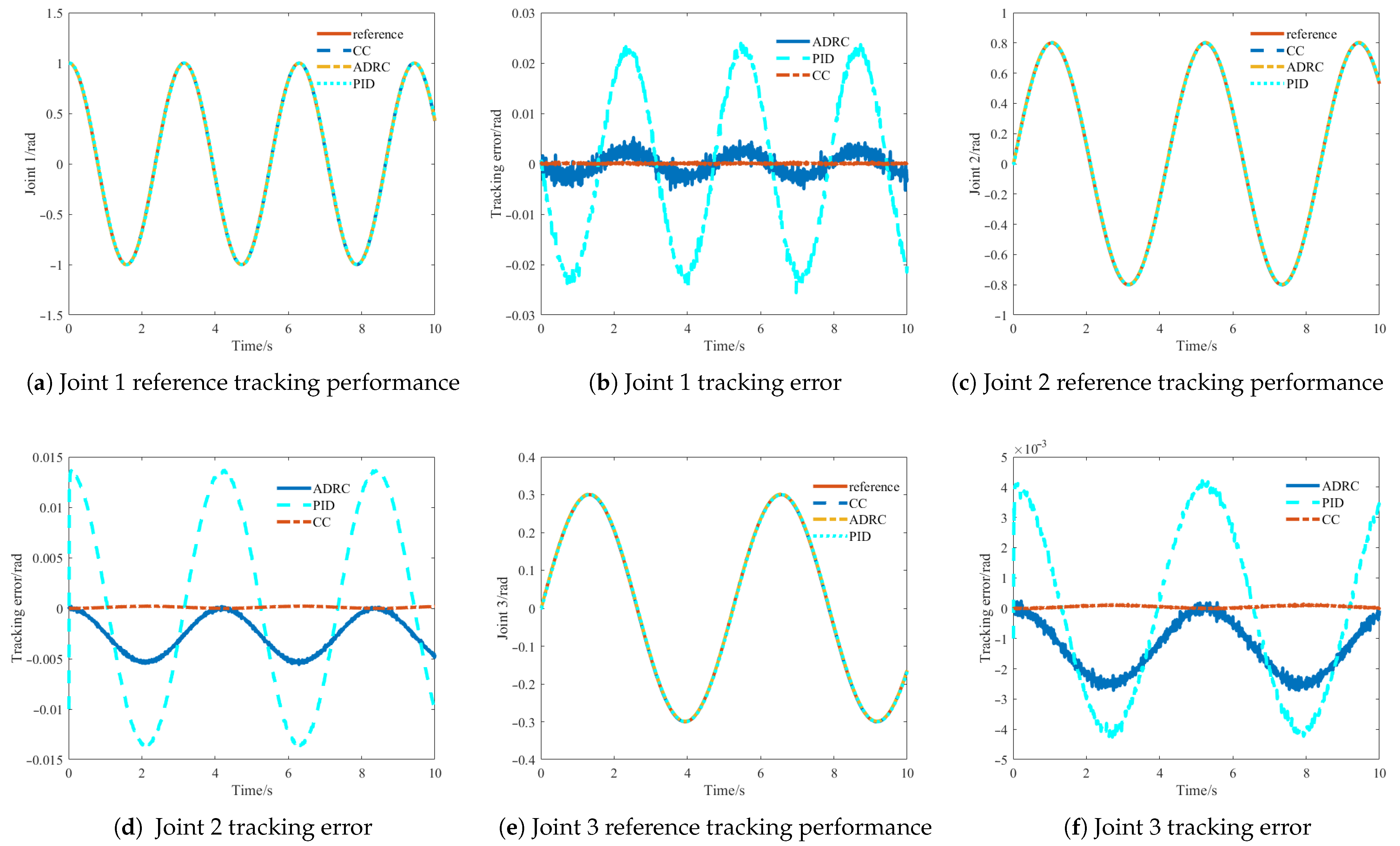
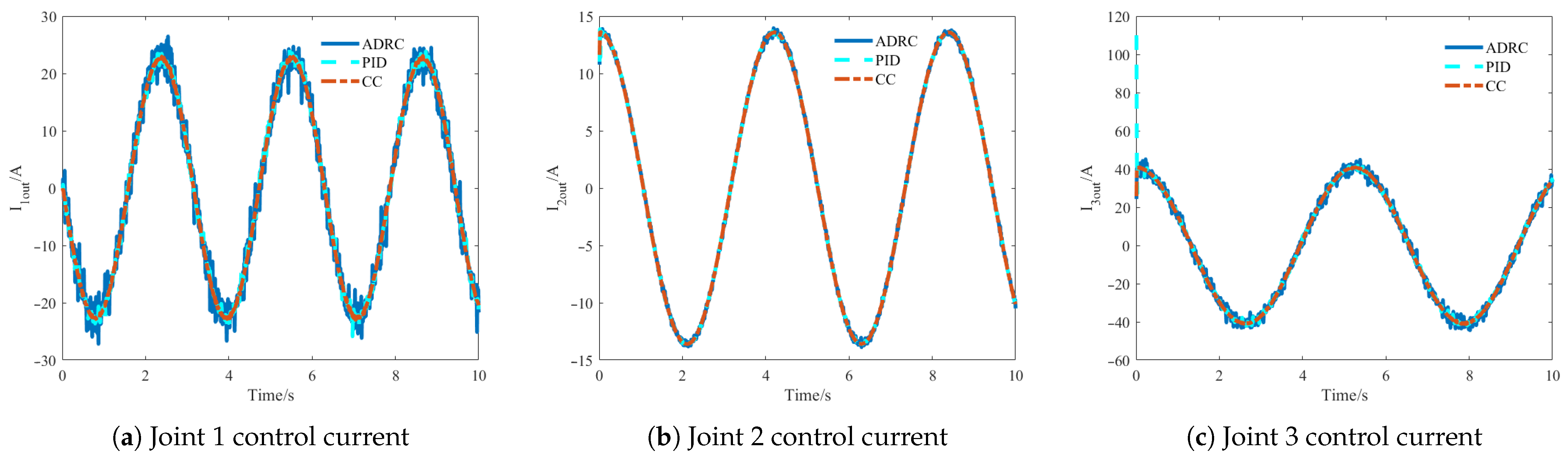
5.1. Trajectory Tracking Comparison Experiment Without Considering Lumped Uncertainties

Under nominal modeling conditions (excluding uncertainties and disturbances), joint tracking performance was experimentally evaluated, with simulation outcomes visualized in Figure 5 and Figure 6. From Figure 5, which compares the tracking performance of the robotic arm under three different control methods, the following can be observed.

Under all three control methods, links 1, 2, and 3 of the robotic arm demonstrate a certain tracking capability for the desired trajectory, but with significant differences in tracking accuracy. Specifically, the CC method shows tracking errors within $\left(0,{10}^{-4}\mathrm{rad}\right)$, $\left(0,2.5\times {10}^{-4}\mathrm{rad}\right)$, and $\left(0,{10}^{-5}\mathrm{rad}\right)$ for links 1, 2, and 3, respectively. The ADRC method exhibits tracking errors within $\left(-0.003\mathrm{rad},0.003\mathrm{rad}\right)$, $\left(-0.006\mathrm{rad},0\right)$, and $\left(-2.5\times {10}^{-3}\mathrm{rad},0\right)$. The PID method demonstrates tracking errors within $(-0.025\mathrm{rad},0.025\mathrm{rad})$, $(-0.015\mathrm{rad},0.015\mathrm{rad})$, and $(-0.005\mathrm{rad},0.005\mathrm{rad})$. These results prove that the CC-controlled robotic arm achieves better tracking performance with higher accuracy compared to both ADRC and PID methods.

Additionally, Figure 6 compares the control currents for all three links under different methods. Without external disturbances, only the PID method shows significant initial fluctuations (within 0.1 s). All three methods maintain relatively stable control currents after 0.1 s. The current curves indicate stable control performance under these conditions for all methods.

5.2. Trajectory Tracking Comparison Experiment Considering Lumped Uncertainties

To further verify the robustness of the CC method and simulate more realistic working conditions, we introduced lumped uncertainties d and $d_1$ into the system, setting them as

$$d=d_1={\left[\begin{array}{ccc}0.001·sint·\mathrm{rand}\left(1\right)\hfill & 0.0001·cost·\mathrm{rand}\left(1\right)\hfill & 0.0001·cost·\mathrm{rand}\left(1\right)\hfill \end{array}\right]}^{\mathrm{T}}$$

(72)

where $\mathrm{rand}\left(1\right)$ represents white noise with an amplitude of 1.

Under identical experimental configurations, with the introduction of lumped uncertainties, the trajectory tracking deviations and control current profiles are, respectively, presented in Figure 7 and Figure 8, while the CC observer’s uncertainty estimation performance is visualized in Figure 9.

Figure 7 demonstrates the trajectory tracking performance under lumped uncertainties. From Figure 7a,c,e, it can be seen that after adding lumped uncertainties, links 1, 2, and 3 of the robotic arm still maintain certain tracking capability for the desired trajectory under all three control methods. However, Figure 7b,d,f reveal significant fluctuations in their tracking errors, with ADRC showing the most pronounced fluctuations, followed by PID, and finally, CC exhibiting the smallest variations. Clearly, even with uncertain disturbances, the CC method’s maximum tracking error still meets steady-state requirements, and its stability outperforms both ADRC and PID methods.

The control current comparison in Figure 8 further reveals the system’s dynamic characteristics. The output control currents of the three methods show that when affected by uncertain disturbances, ADRC and PID methods exhibit obvious and severe fluctuations. These current fluctuations directly translate to motor torque output, causing jitter in the robotic arm’s end-effector. In contrast, the CC method shows much milder current fluctuations under external disturbances, further demonstrating its superiority in terms of output current stability.

Figure 9 reveals the core advantage of the CC method—the observer’s compensation effect on lumped uncertainties. The observer’s disturbance estimation for all three links shows that the estimation error remains below 10% of the original disturbance amplitude. This high-precision real-time estimation capability enables real-time disturbance compensation, fundamentally ensuring the aforementioned tracking accuracy and control stability.

Furthermore, we conducted a more detailed analysis of the simulation results using three metrics [32]: Root Mean Square Error (RMSE), Integral of Absolute Tracking Error Rate (IATER), and Integral of Absolute Output Current Derivative (IAOCD). RMSE and IATER evaluate tracking performance, while IAOCD assesses current output stability. The calculation formulas are as follows:

$$\mathrm{RMSE}=\sqrt{{\displaystyle \frac{1}{10}}{\int }_0^{10}\left(\gamma -{\gamma }_{\mathrm{d}}\right)\mathrm{d}t}$$

(73)

$$\mathrm{IATER}={\int }_0^{10}\left|{\displaystyle \frac{\mathrm{d}\left(\gamma -{\gamma }_{\mathrm{d}}\right)}{\mathrm{d}t}}\right|\mathrm{d}t$$

(74)

$$\mathrm{IAOCD}={\int }_0^{10}\left|{\displaystyle \frac{\mathrm{d}{I}_{\mathrm{out}}}{\mathrm{d}t}}\right|\mathrm{d}t$$

(75)

The calculated results are recorded in

Table 5. Comparison of controller performance with/without external disturbances.

Performance Metrics		RMSE (${10}^{-4}$)			IATER (${10}^{-3}$)			IATER (${10}^5$)
Joint		1	2	3	1	2	3	1	2	3
without disturbances	CC	1.23	1.26	0.63	1.339	1.074	0.408	29.225	13.323	3.200
	ADRC	20.20	31.52	15.67	32.274	26.029	9.810	29.228	13.340	3.202
	PID	158.94	94.43	28.45	292.149	144.915	39.368	29.218	14.483	4.186
with disturbances	CC	1.33	1.29	0.64	5.451	1.4175	1.3806	36.561	13.542	3.972
	ADRC	25.26	35.54	19.35	1374.075	137.547	135.516	237.603	26.401	23.688
	PID	165.34	101.46	30.27	794.665	171.167	85.619	90.693	16.044	9.983

. Taking link 1 as an example for analysis, the RMSE of the robotic arm controlled by the CC method changed from $1.23\times {10}^{-4}$ to $1.33\times {10}^{-4}$ after disturbance addition, remaining essentially unchanged, while the RMSE of the ADRC method increased from $20.20\times {10}^{-4}$ to $25.26\times {10}^{-4}$ and the PID method’s RMSE increased from $158.94\times {10}^{-4}$ to $165.34\times {10}^{-4}$, with ADRC showing the most significant relative change. Regarding IATER, the CC method showed a slight increase from $1.339\times {10}^{-3}$ to $5.451\times {10}^{-3}$, whereas the ADRC and PID methods exhibited drastic increases from $32.274\times {10}^{-3}$ to $1374.075\times {10}^{-3}$ and from 292.149 $\times {10}^{-3}$ to $794.665\times {10}^{-3}$, respectively. This indicates that the CC method’s tracking error remained stable post-disturbance, while the ADRC and PID methods suffered significant precision degradation. For IAOCD, all three methods maintained IAOCD around $29\times {10}^5$ before disturbance, but after disturbance addition, the ADRC and PID methods increased to $237.603\times {10}^5$ and $90.693\times {10}^5$, respectively, in contrast to the CC method’s increase of only $7.3\times {10}^5$. These data demonstrate that the CC method reduced output control force fluctuations by over 40% compared to the PID method, further validating the superior robustness of the CC method.

In conclusion, the CC strategy developed in this study remarkably enhances robotic manipulator trajectory tracking precision. Experimental validation confirms the methodology’s capability to maintain tracking accuracy while demonstrating parametric robustness and external disturbance rejection, with particular efficacy in compensating unmodeled dynamics. Comparative evaluations against conventional ADRC and PID approaches substantiate superior performance in both tracking accuracy and robustness.

6. Conclusions

This study establishes a dual-focused methodology for HDFRAs, developing high-fidelity dynamic models while implementing adaptive trajectory tracking through closed-loop control strategies. First, the dynamic equations of the mechanical subsystem were established using AMM and Lagrange equations, while the hydraulic subsystem model was obtained through fluid continuity equations and Newtonian dynamics. Then, based on SPT, the original model was innovatively decomposed into three subsystems: SRS, SFS, and FHS. According to the distinct dynamic characteristics of each subsystem, AFTSM-ADRC (for SRS/SFS) and SMO-ISMCC (for FHS) were designed, respectively. The newly designed BESO enhances the observation capability and accuracy of the observer, while the novel adaptive sliding mode reaching law effectively suppresses chattering phenomena. Based on Lyapunov stability theory, the global asymptotic stability of the composite control system under lumped uncertainties was rigorously proved.

Numerical simulation results show that (1) regarding trajectory tracking performance, the SPT-based CC method demonstrates significant advantages over conventional ADRC and PID methods, with tracking errors stably converging to the $\left(0,{10}^{-4}\mathrm{rad}\right)$ range, and (2) under white noise disturbances, the system’s output current fluctuations are reduced by over 40% compared to PID control, verifying the strong robustness and stability of the proposed method.

Future research will focus on the following innovative work: (1) extending cross-scale coordinated control strategies to multi-degree-of-freedom robotic arm systems and establishing a unified rigid–flexible–fluid coupled dynamics framework; and (2) constructing a deep reinforcement learning-driven parameter optimization platform to achieve co-optimization of singular perturbation parameters and controller gains.

References

1. Liu, Z.; Sun, J.; Yue, D.; Zuo, X.; Gao, H.; Feng, K. A review on integral evolution of electro-hydraulic actuation in three momentous domains: Aerospace, engineering machinery, and robotics. In Proceedings of the Fourth International Conference on Mechanical Engineering, Intelligent Manufacturing, and Automation Technology (MEMAT 2023), Guilin, China, 20–22 October 2023; Volume 13082, pp. 141–159. [Google Scholar]
2. Kumar, S.B.; Hossem, M.S.; Sayed, A. A Comprehensive Review of Hydraulic Systems in Aerospace and Construction Engineering. Control Syst. Optim. Lett. 2024, 2, 266–273. [Google Scholar] [CrossRef]
3. Vitanov, I.; Farkhatdinov, I.; Denoun, B.; Palermo, F.; Otaran, A.; Brown, J.; Omarali, B.; Abrar, T.; Hansard, M.; Oh, C.; et al. A suite of robotic solutions for nuclear waste decommissioning. Robotics 2021, 10, 112. [Google Scholar] [CrossRef]
4. Wei, X.; Ye, J.; Xu, J.; Tang, Z. Adaptive dynamic programming-based cross-scale control of a hydraulic-driven flexible robotic manipulator. Appl. Sci. 2023, 13, 2890. [Google Scholar] [CrossRef]
5. Chang, W.; Li, Y.; Tong, S. Adaptive fuzzy backstepping tracking control for flexible robotic manipulator. IEEE/CAA J. Autom. Sin. 2018, 8, 1923–1930. [Google Scholar] [CrossRef]
6. Sun, Y.; Wan, Y.; Ma, H.; Liang, X. Real-time force control of hydraulic manipulator arms without force or pressure feedback using a nonlinear algorithm. IEEE Robot. Autom. Lett. 2023, 8, 7146–7153. [Google Scholar] [CrossRef]
7. Peng, J.; Xu, W.; Hu, Z.; Liang, B.; Wu, A. Modeling and analysis of the multiple dynamic coupling effects of a dual-arm space robotic system. Robotica 2020, 38, 2060–2079. [Google Scholar] [CrossRef]
8. Zhang, F.; Yuan, Z. The study of coupling dynamics modeling and characteristic analysis for flexible robots with nonlinear and frictional joints. Arab. J. Sci. Eng. 2022, 47, 15347–15363. [Google Scholar] [CrossRef]
9. Ghorbani, H.; Tarvirdizadeh, B.; Alipour, K.; Hadi, A. Near-time-optimal motion control for flexible-link systems using absolute nodal coordinates formulation. Mech. Mach. Theory 2019, 140, 686–710. [Google Scholar] [CrossRef]
10. Wang, B.L.; Cai, Y.; Song, J.C.; Sepehri, N. LuGre model–based robust adaptive control for a pump-controlled hydraulic actuator experiencing friction. Trans. Inst. Meas. Control 2024, 46, 1845–1857. [Google Scholar] [CrossRef]
11. Kelkar, R.; Santhya, M.; Kanchan, M.; Powar, O.S. Bond Graph Modeling and Simulation of Hybrid Piezo-Flexural-Hydraulic Actuator. Eng. Proc. 2024, 59, 202. [Google Scholar]
12. Xie, Q.; Wang, T.; Zhu, S. Simplified dynamical model and experimental verification of an underwater hydraulic soft robotic arm. Smart Mater. Struct. 2022, 31, 075011. [Google Scholar] [CrossRef]
13. Mehrez, M.W.; El-Badawy, A.A. Effect of the joint inertia on selection of under-actuated control algorithm for flexible-link manipulators. Mech. Mach. Theory 2010, 45, 967–980. [Google Scholar] [CrossRef]
14. Xu, B.; Yuan, Y. Two performance enhanced control of flexible-link manipulator with system uncertainty and disturbances. Sci. China Inf. Sci. 2017, 60, 050202. [Google Scholar] [CrossRef]
15. Wang, C.; Quan, L.; Zhang, S.; Meng, H.; Lan, Y. Reduced-order model based active disturbance rejection control of hydraulic servo system with singular value perturbation theory. ISA Trans. 2017, 67, 455–465. [Google Scholar] [CrossRef]
16. Yao, J.; Deng, W.; Jiao, Z. RISE-based adaptive control of hydraulic systems with asymptotic tracking. IEEE Trans. Autom. Sci. Eng. 2015, 14, 1524–1531. [Google Scholar] [CrossRef]
17. Yao, J.; Deng, W. Active disturbance rejection adaptive control of hydraulic servo systems. IEEE Trans. Ind. Electron. 2017, 64, 8023–8032. [Google Scholar] [CrossRef]
18. Deng, W.; Yao, J. Asymptotic tracking control of mechanical servosystems with mismatched uncertainties. IEEE/ASME Trans. Mechatronics 2020, 26, 2204–2214. [Google Scholar] [CrossRef]
19. Won, D.; Kim, W.; Tomizuka, M. High-gain-observer-based integral sliding mode control for position tracking of electrohydraulic servo systems. IEEE/ASME Trans. Mechatronics 2017, 22, 2695–2704. [Google Scholar] [CrossRef]
20. Barhaghtalab, M.H.; Meigoli, V.; Haghighi, M.R.G.; Nayeri, S.A.; Ebrahimi, A. Dynamic analysis, simulation, and control of a 6-DOF IRB-120 robot manipulator using sliding mode control and boundary layer method. Methods 2018, 11, 12. [Google Scholar] [CrossRef]
21. Ma, T.; Guo, X.; Su, G.; Deng, H.; Yang, T. Research on synchronous control of active disturbance rejection position of multiple hydraulic cylinders of digging-anchor-support robot. Sensors 2023, 23, 4092. [Google Scholar] [CrossRef]
22. Chen, Z.; Zhou, S.; Shen, C.; Lyu, L.; Zhang, J.; Yao, B. Observer-based adaptive robust precision motion control of a multi-joint hydraulic manipulator. IEEE/CAA J. Autom. Sin. 2024, 11, 1213–1226. [Google Scholar] [CrossRef]
23. Wang, B.L.; Cai, Y.; Song, J.C.; Liang, Q.K. A Singular Perturbation Theory-Based Composite Control Design for a Pump-Controlled Hydraulic Actuator with Position Tracking Error Constraint. Actuators 2023, 12, 265. [Google Scholar] [CrossRef]
24. Su, Y.; Müller, P.C.; Zheng, C. Global asymptotic saturated PID control for robot manipulators. IEEE Trans. Control Syst. Technol. 2009, 18, 1280–1288. [Google Scholar] [CrossRef]
25. Di Gregorio, R. A geometric and analytic technique for studying multi-DOF planar mechanisms’ dynamics. Mech. Mach. Theory 2022, 176, 104975. [Google Scholar] [CrossRef]
26. Kong, X.; Cai, B.; Liu, Y.; Zhu, H.; Liu, Y.; Shao, H.; Yang, C.; Li, H.; Mo, T. Optimal sensor placement methodology of hydraulic control system for fault diagnosis. Mech. Syst. Signal Process. 2022, 174, 109069. [Google Scholar] [CrossRef]
27. Zhou, L.; Li, Z.; Yang, H.; Tan, C.; Fu, Y. Adaptive Terminal Sliding Mode Control for High-Speed EMU: A MIMO Data-Driven Approach. IEEE Trans. Autom. Sci. Eng. 2025, 22, 1970–1983. [Google Scholar] [CrossRef]
28. Wu, L.; Liu, J.; Vazquez, S.; Mazumder, S.K. Sliding mode control in power converters and drives: A review. IEEE/CAA J. Autom. Sin. 2021, 9, 392–406. [Google Scholar] [CrossRef]
29. Huang, X.; Lin, W.; Yang, B. Global finite-time stabilization of a class of uncertain nonlinear systems. Automatica 2005, 41, 881–888. [Google Scholar] [CrossRef]
30. Wang, Q.; Lu, G.; Zhao, M.; Sun, J. Finite-time stability and stabilization of discrete-time hybrid systems. Syst. Control Lett. 2024, 189, 105832. [Google Scholar] [CrossRef]
31. Zhou, L.; Li, Z.-Q.; Yang, H.; Tan, C. Integral predictive sliding mode control for high-speed trains: A dynamic linearization and input constraint-based data-driven scheme. Control. Eng. Pract. 2025, 154, 106139. [Google Scholar] [CrossRef]
32. Xu, J.; Sui, Z.; Wang, W.; Xu, F. An adaptive discrete integral terminal sliding mode control method for a Two-Joint manipulator. Processes 2024, 12, 1106. [Google Scholar] [CrossRef]
Figure 1. Schematic diagram of the HDFRA structure.
Processes 13 01805 g001
Figure 2. Simplified diagram of a 3-DOF robotic arm.
Processes 13 01805 g002
Figure 3. Configuration of differential area hydraulic actuator.
Processes 13 01805 g003
Figure 4. Block diagram of HDFRAs with controllers.
Processes 13 01805 g004
Figure 5. Comparison of tracking performance for the robotic arm controlled by three different methods under nominal conditions (without considering lumped uncertainties).
Processes 13 01805 g005
Figure 6. Comparison of control current outputs for the robotic arm under three different control methods under nominal conditions (without lumped uncertainties).
Processes 13 01805 g006
Figure 7. Tracking performance comparison of the robotic arm under three control methods with lumped uncertainties considered.
Processes 13 01805 g007
Figure 8. Control current output comparison of the robotic arm under three control methods with lumped uncertainties considered.
Processes 13 01805 g008
Figure 9. Observation of lumped uncertainties by the CC method.
Processes 13 01805 g009