Solubility Prediction in N₂O + Ionic Liquid Systems Using Artificial Neural Networks Including Thermodynamically Consistent Data

Abstract

The solubilities of 498 datasets of N₂O and ionic liquid systems were predicted using a multilayer perceptron. The data used to train the artificial neural network was subjected to the Gibbs–Duhem test to analyze their thermodynamic consistency. The Peng–Robinson cubic equation of state, combined with the Kwak–Mansoori mixing rule, was used as the thermodynamic model to implement the test. The analysis indicated that 71.9% of the data were declared thermodynamically inconsistent. The ability of artificial neural networks (ANNs) to predict the solubility of these systems using experimental datasets that do not satisfy the thermodynamic consistency criteria based on the Gibbs–Duhem equation was studied. The multilayer perceptron model achieved an average absolute deviation of 1.81% and a maximum individual deviation of 7.56%. These results highlight the potential of ANNs as robust predictive tools even when the available data do not fully satisfy thermodynamic consistency criteria.

1. Introduction

Growing concerns about global warming caused by greenhouse gas (GHG) emissions from fossil fuel combustion have driven the development of technologies to reduce and capture these gases. The main GHGs in the Earth’s atmosphere include carbon dioxide (CO₂), methane (CH₄), sulfur dioxide (SO₂), and nitrous oxide (N₂O).

Significant attention has been paid to CO₂ emissions being among the main drivers of global warming [1,2,3]. The climate threats caused by atmospheric CO₂ have prompted a global commitment to reduce emissions. However, the levels of other GHGs such as nitrous oxide (N₂O) have also increased, with a 23% increase between 1750 and 2019 [4]. N₂O has a global warming potential approximately 310 times greater than that of CO₂ when normalized over 100 years [5].

N₂O is produced from both natural and anthropogenic sources. The main source of N₂O emissions is agricultural activity, which accounts for approximately 60% of total emissions [6,7]. Industrial sources include adipic acid production (a raw material for nylon), nitric acid production, fossil fuel power plants, vehicular emissions, and explosives manufacturing [8,9]. In these processes, N₂O is a residual product that is diverted to the atmosphere. Although a variety of technologies are used to reduce N₂O emissions from adipic acid production, these technologies cannot be applied to other N₂O emission sources, such as nitric acid production, because of the relatively low concentration of N₂O in the gas stream [10].

To address this problem, various gas capture and storage technologies have been developed. Among these, the most promising are ionic liquids (ILs), which are chemical compounds consisting of ions that are in a liquid state at room temperature [11,12,13,14,15]. They have a high affinity for gases, low flammability and toxicity, and high thermal stability, and can absorb large amounts of gas into their structure. Consequently, ILs help reduce the emissions of polluting gases into the atmosphere and are therefore considered green solvents [1,16,17,18]).

This has led to growing interest in the study of ILs as solvents in gas separation processes and the capture of pollutants such as CO₂, CH₄, SO₂, and N₂O [1,19,20,21]. ILs have demonstrated a high capacity to absorb N₂O, thus prompting numerous experimental solubility studies characterizing the vapor–liquid equilibrium (VLE) of N₂O + IL systems. Shiflett et al. (2012) studied the separation of N₂O and CO₂ in [bmim][Ac] between 283 and 348 K and up to 2 MPa using a gravimetric microbalance determining VLE data [22]. Shiflett et al. (2012) measured the solubility of N₂O in six ILs at temperatures between 283 and 348 K and pressures up to 2 MPa using a Hiden IGA 003 gravimetric microbalance [23]. In both studies, the instrumental uncertainty in temperature was ±0.1 K, that in pressure was ±0.8 kPa, and that in molar fraction of solubility was <0.006. Revelli et al. (2010) examined the solubility of N₂O in five ILs to evaluate the efficiency of emissions over a wide range of pressures up to 300 bar and temperatures between 293 and 373 K using a variable-volume cell and synthetic method. The temperature was measured with an accuracy of ±0.1 K, and the pressure was with 0.1 bar [24].

However, despite the growing amount of VLE data available, the high costs associated with obtaining ILs have encouraged the complementary use of models capable of extrapolating the thermodynamic behavior of N₂O + ILs mixtures to broader temperature and pressure conditions. These models range from classical ones based on equations of state (EoS) and activity coefficients to recent ones based on artificial intelligence. Amar et al. (2021) trained a model using a cascading forward neural network (CFNN), a radial basis function neural network (RBFNN), and gene expression programming (GEP) on experimental data to predict the solubility of N₂O in ILs [13]. The best performance was obtained by CFNN-LM [13]. Shaahmadi et al. (2017) compiled N₂O–ionic liquid solubility data to evaluate the performance of three intelligent models for predicting N₂O absorption. Their results show good agreement between model estimates and experimental measurements, supporting their potential use in process design [25]. Feng et al. (2023) applied the voting method (VM) with five algorithms and a two-layer feed-forward neural network (TLFFNN) method to predict the solubility of N₂O + LI mixtures. Their findings showed that the TLFFNN method achieved the highest accuracy, with an R² = 0.9981, for the design of ILs optimized for N₂O removal [26].

Models based on ANNs have performed excellently in predicting solubility for gas-IL systems, thereby achieving acceptable predictions over a wide range of temperatures and pressures [27,28,29]. These results are due to the ability of ANNs to capture nonlinear relationships and learn complex patterns from experimental data; this ability enables ANN to reproduce equilibrium behavior with good accuracy.

Among the most widely used ANN models is the multilayer perceptron (MLP), which has been extensively documented in the literature [30,31,32]. On the basis of a set of input variables, the model adjusts the parameters of the ANN to predict a specific output [33]. The predictive capacity of MLPs depends mainly on the training dataset and does not require an explicit thermodynamic description of the system [25,26]. This raises a key question: To what extent does the performance of ANN-based models depend on the quality and thermodynamic consistency of the data used for training and validation?

Thermodynamics provides fundamental tools that allow for the quality of a set of equilibrium data to be evaluated. One of the most widely applied methods is the consistency test based on the Gibbs–Duhem equation [34]. In general terms, the Gibbs–Dohme consistency test compares experimentally measured and predicted behaviors by using a thermodynamic model and evaluates discrepancies through an area test. On the basis of criteria predefined in the literature, datasets can be classified into three categories: thermodynamically consistent (TC), not fully consistent (NFC), or thermodynamically inconsistent (TI). This classification helps determine which datasets are suitable for modeling a system composed of binary mixtures [35,36].

In this work, we evaluate the ability of ANN models to predict the solubility of N₂O in ionic liquids using experimental datasets that do not satisfy thermodynamic consistency criteria based on the Gibbs–Duhem equation. Four hundred ninety-eight experimental data points from binary N₂O + IL systems reported in the literature were subjected to a thermodynamic consistency test based on the Gibbs–Duhem equation and the Peng–Robinson cubic equation of state with the Kwak and Mansoori mixing rule (PR/KM EoS). As a result of the test, 71.9% of the total data were classified as thermodynamically inconsistent. The total dataset was subsequently used to train an MLP model to predict solubility. The findings show that the ANN performed excellently in the training, validation, and prediction stages, thereby demonstrating its ability to predict solubility behavior, even with data that are thermodynamically inconsistent.

2. Materials and Methods

2.1. Gibbs–Duhem Consistency Test

Starting from the fundamental Gibbs–Duhem equation expressed in terms of fugacity coefficients, we obtain the following relationship [37]:

$$\sum {\mathit{x}}_{\mathit{i}} \mathit{d}\mathit{l}\mathit{n}{\mathit{\phi }}_{\mathit{i}} = -{\displaystyle \frac{{\mathit{H}}^{\mathit{R}}}{\mathit{R}{\mathit{T}}^2}} \mathit{d}\mathit{T} + {\displaystyle \frac{{\mathit{V}}^{\mathit{R}}}{\mathit{R}\mathit{T}}} \mathit{d}\mathit{P}$$

(1)

At constant temperature, Equation (1) reduces to

$$\int {\displaystyle \frac{1}{\mathit{P}{\mathit{x}}_1}}\mathit{d}\mathit{P}=\int {\displaystyle \frac{1}{\left(\mathit{Z}-1\right){\mathit{\phi }}_1}}\mathit{d}{\mathit{\phi }}_1+\int {\displaystyle \frac{1-{\mathit{x}}_1}{{\mathit{x}}_1\left(\mathit{Z}-1\right){\mathit{\phi }}_2}}\mathit{d}{\mathit{\phi }}_2$$

(2)

where the left side of Equation (2) defines an area (A_p) determined using experimental solubility data for N₂O in ILs at a fixed temperature. The right side of Equation (2) defines an area (Aφ) calculated using a thermodynamic model.

The percentage deviation in areas is calculated as follows:

$$∆{\mathit{A}}_{\mathit{i}}\mathit{\%}=100{\sum }_{\mathit{i}=1}^{\mathit{N}}{\left({\displaystyle \frac{{\mathit{A}}_{\mathit{\phi }}-{\mathit{A}}_{\mathit{P}}}{{\mathit{A}}_{\mathit{P}}}}\right)}_{\mathit{i}}$$

(3)

$$\left|∆{\mathit{A}}_{\mathit{i}}\mathit{\%}\right|=100 {\sum }_{\mathit{i}=1}^{\mathit{N}}{\left|{\displaystyle \frac{{\mathit{A}}_{\mathit{\phi }}-{\mathit{A}}_{\mathit{P}}}{{\mathit{A}}_{\mathit{P}}}}\right|}_{\mathit{i}}$$

(4)

The maximum deviations for $∆{\mathit{A}}_{\mathit{i}}\mathit{\%}$ were defined in the range −20% to +20%. A dataset is considered thermodynamically consistent (TC) when the value of |∆A|_i% (Equation (3)) is less than 20%. However, if only 25% of the original points do not meet this criterion, the original dataset is declared not fully consistent (NFC). Finally, if neither condition is satisfied, the set is declared thermodynamically inconsistent (TI). Further details on the consistency criteria have been presented in previous works [35,36].

2.2. PR/KM Thermodynamical Model

The Peng–Robinson (PR) equation of state is given by the following [38]:

$$\mathit{P}={\displaystyle \frac{\mathit{R}\mathit{T}}{\left(\mathit{V}-\mathit{b}\right)}}-{\displaystyle \frac{\mathit{c}+\mathit{R}\mathit{T}-2\sqrt{\mathit{c}\mathit{d}\mathit{R}\mathit{T}}}{\mathit{V}\left(\mathit{V}+\mathit{d}\right)+\mathit{b}\left(\mathit{V}-\mathit{b}\right)}}$$

(5)

For mixtures, the modified equation with the Kwak–Mansoori mixing rule (PR/KM) is as follows [39]:

$$\mathit{P}={\displaystyle \frac{\mathit{R}\mathit{T}}{\mathit{V}-{\mathit{b}}_{\mathit{m}}}}-{\displaystyle \frac{{\mathit{c}}_{\mathit{m}}+\mathit{R}\mathit{T}{\mathit{d}}_{\mathit{m}}-2\sqrt{\mathit{R}\mathit{T}{\mathit{c}}_{\mathit{m}}{\mathit{d}}_{\mathit{m}}}}{\mathit{V}\left(\mathit{V}+{\mathit{b}}_{\mathit{m}}\right)+\mathit{b}\left(\mathit{V}-{\mathit{b}}_{\mathit{m}}\right)}}$$

(6)

The mixing and combining rules proposed by Kwak and Mansoori for Equations (5) and (6) are shown in Table 1. In these equations, ${\mathit{x}}_{\mathit{i}}$ denotes the mole fraction of component $\mathit{i}$ in the liquid or vapor phase. The PR/KM model contains up to three adjustable binary parameters (${\mathit{k}}_{\mathit{i}\mathit{j}}$, ${\mathit{l}}_{\mathit{i}\mathit{j}}$, ${\mathit{m}}_{\mathit{i}\mathit{j}}$), one associated with each constant, and they are assumed to be identical in both phases, i.e., liquid and vapor. Additionally, the model requires the critical properties (${\mathit{T}}_{\mathit{c}}$ and ${\mathit{P}}_{\mathit{c}}$) and the acentric factor ($\mathit{\omega }$) for each component in the mixture.

Table 1. Parameters of the PR and PR/KM models.

PR Parameters			PR\KM Parameters
$\mathit{c}$	$=$	${\mathit{a}}_{\mathit{c}}\left(1+{\mathit{F}}^2\right)$	${\mathit{c}}_{\mathit{m}}$	$=$	${\displaystyle \sum _{\mathit{i}}}{\displaystyle \sum _{\mathit{j}}}{\mathit{x}}_{\mathit{i}}{\mathit{x}}_{\mathit{j}}{\mathit{c}}_{\mathit{i}\mathit{j}}$	${\mathit{b}}_{\mathit{i}}$	$=$	$0.0778{\displaystyle \frac{\mathit{R}{\mathit{T}}_{\mathit{c}\mathit{i}}}{{\mathit{P}}_{\mathit{c}\mathit{i}}}}$
${\mathit{a}}_{\mathit{c}}$	$=$	$0.4572{\displaystyle \frac{{\mathit{R}}^2{\mathit{T}}_{\mathit{c}}^2}{{\mathit{P}}_{\mathit{c}}}}$	${\mathit{c}}_{\mathit{i}\mathit{j}}$	$=$	$\sqrt{{\mathit{c}}_{\mathit{i}}{\mathit{c}}_{\mathit{j}}}\left(1-{\mathit{k}}_{\mathit{i}\mathit{j}}\right)$	${\mathit{d}}_{\mathit{m}}$	$=$	${\displaystyle \sum _{\mathit{i}}}{\displaystyle \sum _{\mathit{j}}}{\mathit{x}}_{\mathit{i}}{\mathit{x}}_{\mathit{j}}{\mathit{d}}_{\mathit{i}\mathit{j}}$
$\mathit{F}$	$=$	$0.3746+1.5423 \mathit{\omega }-0.2699 {\mathit{\omega }}^2$	${\mathit{c}}_{\mathit{i}}$	$=$	${\mathit{c}}_{\mathit{c}\mathit{i}}\left(1+{\mathit{F}}_{\mathit{i}}^2\right)$	${\mathit{d}}_{\mathit{i}\mathit{j}}$	$=$	$\left({\displaystyle \frac{{\mathit{d}}_{\mathit{i}}^{\frac{1}{3}}+{\mathit{d}}_{\mathit{j}}^{\frac{1}{3}}}{2}}\right)\left(1-{\mathit{m}}_{\mathit{i}\mathit{j}}\right)$
$\mathit{b}$	$=$	$0.0778{\displaystyle \frac{\mathit{R}{\mathit{T}}_{\mathit{c}}}{{\mathit{P}}_{\mathit{c}}}}$	${\mathit{b}}_{\mathit{m}}$	$=$	${\displaystyle \sum _{\mathit{i}}}{\displaystyle \sum _{\mathit{j}}}{\mathit{x}}_{\mathit{i}}{\mathit{x}}_{\mathit{j}}{\mathit{b}}_{\mathit{i}\mathit{j}}$	${\mathit{d}}_{\mathit{i}}$	$=$	${\displaystyle \frac{\mathit{a}\left({\mathit{T}}_{\mathit{c}\mathit{i}}\right){\mathit{F}}^2}{\mathit{R}{\mathit{T}}_{\mathit{c}\mathit{i}}}}$
$\mathit{d}$	$=$	${\displaystyle \frac{{\mathit{a}}_{\mathit{c}}{\mathit{F}}^2}{\mathit{R}{\mathit{T}}_{\mathit{c}}}}$	${\mathit{b}}_{\mathit{i}\mathit{j}}$	$=$	$\left({\displaystyle \frac{{\mathit{b}}_{\mathit{i}}^{\frac{1}{3}}+{\mathit{b}}_{\mathit{j}}^{\frac{1}{3}}}{2}}\right)\left(1-{\mathit{l}}_{\mathit{i}\mathit{j}}\right)$

The accuracy of the model in correlating VLE experimental data is determined by calculating the relative deviation in the correlated pressure (ΔP%) and the absolute deviation in the correlated pressure (|ΔP%|). This deviation is defined as follows:

$$\mathbf{\Delta }\mathit{P}\mathit{\%}={\displaystyle \frac{100}{\mathit{N}}}\sum {\left({\displaystyle \frac{{\mathit{P}}^{\mathit{c}\mathit{a}\mathit{l}}-{\mathit{P}}_{\mathit{i}}^{\mathit{e}\mathit{x}\mathit{p}}}{{\mathit{P}}_{\mathit{i}}^{\mathit{e}\mathit{x}\mathit{p}}}}\right)}_{\mathit{i}}$$

(7)

$$\left|\mathbf{\Delta }\mathit{P}\mathit{\%}\right|={\displaystyle \frac{100}{\mathit{N}}}\sum {\displaystyle \frac{{\left|{\mathit{P}}^{\mathit{c}\mathit{a}\mathit{l}}-{\mathit{P}}^{\mathit{e}\mathit{x}\mathit{p}}\right|}_{\mathit{i}}}{{\mathit{P}}_{\mathit{i}}^{\mathit{e}\mathit{x}\mathit{p}}}}$$

(8)

The model is considered acceptable when the correlation between the data is in the range $\left[-10\mathit{\%}, +10\mathit{\%}\right]$. The percentages defined for the consistency criterion and the thermodynamic model are based on information reported in the literature. According to Valderrama and Álvarez (2004), the concentration of the solute in the gas phase can be correlated with higher accuracy using the modified Kwak–Mansoori combining rules [36].

2.3. Solubility Modeling Using a Multilayer Perceptron

The multilayer perceptron (MLP) is a prediction model based on an ANN. This model employs hidden layers with a nonlinear activation functional ${{\mathit{a}}_{\mathit{l}}}^{\mathit{k}+1}$ and a linear output layer. The mapping corresponds to the composition of affine and nonlinear transformations [33].

The data are processed by means of connections between all the neurons in one layer and all the neurons in the next layer. The output of the l-neuron in the hidden layer (k + 1) of a network with M layers is given by Equation (9).

$${a_l}^{k+1}=f^{k+1}\left(\sum _{j=1}^{N_k}{w_{lj}}^{k+1}{a_l}^k+{b_l}^{k+1}\right);k=\mathrm{1,2},3.\dots .\left(M-1\right)$$

(9)

The parameter adjustment is formulated as a least-squares problem. A cost function must first be defined and then minimized via a learning algorithm that iteratively updates the values of the parameters. Additionally, convergence criteria are established.

The selection of input variables considerably influences the training and the extrapolation capacity of the model. The choice of input variables must appropriately represent the phenomenon while bypassing redundancies or nonrepresentative correlations. The performance of MLPs can be evaluated in terms of the individual relative deviation, average relative deviation, and average absolute deviation.

The individual absolute deviation, average absolute deviation, and average relative deviation of each solubility calculated with respect to the experimental data are determined using Equations (10)–(12), respectively.

$$\left|∆x\%\right|=\sum _{i=1}^N\left({\displaystyle \frac{x_i^{cal}-x_i^{exp}}{x_i^{exp}}}\right)$$

(10)

$$\left|∆\stackrel{-}{x_1}\%\right|={\displaystyle \frac{100}{N}}\sum _{i=1}^N\left|{\displaystyle \frac{x_i^{cal}-x_i^{exp}}{x_i^{exp}}}\right|$$

(11)

$$∆\stackrel{-}{x_1}\%={\displaystyle \frac{100}{N}}\sum _{i=1}^N\left({\displaystyle \frac{x_i^{cal}-x_i^{exp}}{x_i^{exp}}}\right)$$

(12)

3. Results

3.1. Consistency Test Results

In this work, seven binary systems composed of N₂O in different ILs were studied: [BMIM][Ac], [BMIM][SCN], [BMIM][BF₄], [BMIM][TF₂N], [DMIM][MP], [(OH)₂IM][TF₂N], and [(ETO)₂IM][TF₂N]. The properties of all the substances considered in this study are listed in Table 2, where M denotes the molecular weight, Tc denotes the critical temperature, P_c denotes the critical pressure, V_c denotes the critical volume, and ω denotes the acentric factor. The values for these properties were taken from Valderrama et al. (2015) [40]. The value ranges of the properties considered were 283 K–348 K for temperature, 0.253 MPa–24.07 MPa for pressures, and 0.002–0.781 for solubility. This study includes 498 experimental data points (P-T-x data). Table 3 presents the temperature, pressure, and solubility ranges used in this work and indicates the bibliographic sources from which the experimental data were obtained.

Table 2. Critical properties, acentric factors, and compressibility factors of all the substances used in this study [40].

Components	M	Tc /K	Pc /Mpa	Vc (cm3/mol)	ω
N2O	44.01	309.57	7.245	27.4	0.1409
[BMIM][AC]	198.3	847.3	2.445	658.2	0.6681
[BMIM][SCN]	197.3	1047.4	1.94	780.7	0.4781
[BMIM][BF4]	226	643.2	2.04	655.0	0.8877
[BMIM][Tf2N]	419.4	1269.9	2.765	990.1	0.3004
[DMIM][MP]	191.1	776.8	3.265	544.4	0.5106
[(ETO)2IM[Tf2N]	437.3	1310.8	2.82	964.2	0.2817
[(OH)2IM[Tf2N]	381.2	1314.1	4.509	746.0	0.7267

Table 3. Systems considered in this work.

System	N	T(K)			P(MPa)			x1			Reference
[BMIM][Ac]	46	283	-	348	0.5006	-	1.9999	0.002	-	0.207	[22]
[BMIM][BF4]	45	292.45	-	373.55	1.140	-	13.330	0.101	-	0.371	[23]
[BMIM][ Tf2N]	56	283.10	-	348.20	0.253	-	2.0006	0.002	-	0.490
[BMIM][SCN]	49	293.05	-	373.30	1.0300	-	18.4900	0.029	-	0.294	[24]
[(OH)2IM][Tf2N]	48	302.85	-	363.15	1.02	-	24.07	0.152	-	0.610
[BMIM][BF4]	40	298.10	-	348.10	0.026	-	2.053	0.002	-	0.208
[(ETO)2IM][Tf2N]	101	302.05	-	363.45	0.610	-	23.30	0.119	-	0.694
[DMIM][MP]	42	293.35	-	373.15	2.100	-	16.450	0.087	-	0.253

The solubilities of N₂O in various ILs were analyzed to assess their thermodynamic consistency. Thirty-nine experimental data points were declared thermodynamically consistent (TC) through tests based on the fundamental Gibbs–Duhem equation and the PR/KM model. For example, for the N₂O + [BMIM][BF₄] system at T = 303 K, the average absolute deviation in pressure is 0.6% in the modeling stage, and the area test yields a value of 6.4%, so the data are classified as TC. As shown in Figure 1a, all n data points considered present relative pressure deviations within 10%, and Figure 1b indicates that the (n − 1) points considered in the consistency test do not exceed the relative deviations of 12% during the area test.

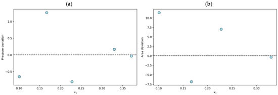
Figure 1. Results for the N₂O + [BMIM][BF₄] system at T = 303 K declared to be thermodynamically consistent (TC): (a) individual relative deviation in pressure for each n-data; (b) individual relative deviation in the area test for each (n − 1)-data.

On the other hand, eighty-one experimental data points were classified as not fully consistent (NFC). For example, the N₂O + [(ETO)₂IM][TF₂N] system at T = 353 K shows an average absolute deviation in pressure of 1.5%, and the average absolute deviation in the area test is 18.3%. As shown in Figure 2a, the n-point subjected to the PR/KM model is within the established limits. However, one of the (n − 1)-points in the set reaches a deviation of 45.3%, and the other point reaches 91.1%; therefore, the data are declared NFC. The results obtained for each of the (n − 1)-points considered during the area test for this system are shown in Figure 2b.

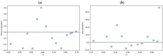
Figure 2. Results for the N₂O + [(ETO)2IM][TF₂N] system at T = 353 K declared to be not fully consistent (NFC): (a) individual relative deviation in pressure for each n-data; (b) individual relative deviation in the area test for each (n − 1)-data.

Finally, three hundred and seven experimental data points were declared thermodynamically inconsistent (TI). One example is the N₂O + [BMIM][TF₂N] mixture at T = 348 K, which shows an average absolute pressure deviation of 9.4% and a result of 17.6% in the area test. This finding indicates that the n-point deviations in the modeling stage are less than 10%. However, the results of the area test reveal that the data are thermodynamically inconsistent. The individual relative deviations in the modeling and the results of the area test for the N₂O + [BMIM][TF₂N] mixture at T = 348 K are shown in Figure 3.

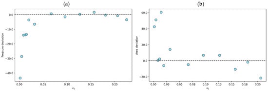
Figure 3. Results or the N₂O + [BMIM][ TF₂N] system at T = 348 K declared to be thermodynamically inconsistent (TI): (a) individual relative deviation in pressure for each n-data; (b) individual relative deviation in the area test for each (n − 1)-data.

The implementation of the consistency test revealed that 9.1% were classified as TC, 19.0% as NFC, and 71.9% as TI. Under these criteria, the dataset is unsuitable for the thermodynamic modeling of solubility. The adjustable parameters, the average absolute deviation, and the maximum individual deviation in pressure for the model and area test results of each dataset are presented in Table 4. The distribution of the thermodynamic consistency test results for all the N₂O + IL mixtures obtained using the PR/KM model are shown in Figure 4.

Table 4. Parameters of the model obtained with the PK/KM model for each dataset considered in this study.

System	N	T(K)	k12	l12	m12	∣ΔP%∣	Δ Pmax%	∣ΔA%∣	Results
[bmim][Ac]	7	283	0.10699	−0.34943	0.46285	2.5	−9.1	12.9	NFC
	13	298	1.16562	−0.24713	1.90768	4.2	20.8	10.0	TI
	13	323	0.48313	−0.35071	1.04085	3.1	−6.7	21.5	TI
	13	348	0.35561	−0.37022	0.87203	7.3	−14.5	19.0	TI
[bmim][SCN]	5	293	0.17330	−0.50775	0.51394	12.0	−47.8	63.7	TI
	5	303	0.43787	−0.50890	0.93237	10.1	−45.9	47.5	TI
	5	313	−0.19714	−0.47808	−0.17994	13.0	−49.7	60.7	TI
	6	323	−0.15897	−0.53200	0.03001	11.7	−43.7	98.2	TI
	5	333	−0.20790	−0.52318	−0.06976	11.8	−46.2	1330.7	TI
	6	343	−0.97160	−0.08639	−2.61700	12.4	−40.8	107.2	TI
	6	353	−0.89860	−0.18553	−2.13983	12.8	−47.0	377.2	TI
	5	363	−0.16380	−0.54426	0.04038	7.1	17.6	151.4	TI
	6	373	0.00062	−0.56128	0.31955	15.9	−46.1	181.2	TI
[(OH)2IM[Tf2N]	7	303	−0.09705	−0.28238	0.31165	1.3	3.4	15.0	TC
	7	313	0.16375	−0.29260	0.76311	3.5	−6.4	16.9	TI
	7	323	−0.48505	−0.22071	−0.51024	6.8	14.1	24.7	TI
	7	333	−0.09517	−0.28073	0.32854	1.8	−3.9	19.9	NFC
	7	343	−1.11403	−0.01150	−2.26711	1.3	3.1	15.7	TC
	7	353	0.24928	−0.28415	0.87042	1.3	−2.8	26.8	NFC
	6	363	−1.16924	0.01409	−2.36537	0.5	−1.3	5.3	TC
[bmim][BF4]	5	293	−1.45067	0.30596	−3.46338	0.9	1.6	7.8	TC
	5	303	−1.46433	0.42253	−3.68356	0.6	1.3	6.4	TC
	5	313	−1.45059	0.43593	−3.58840	1.1	−1.7	6.8	TC
	5	323	−1.43495	0.29647	−3.16127	2.3	−3.1	12.3	TI
	5	333	−1.39647	0.23769	−2.90028	2.7	5.7	15.9	TI
	5	343	−1.38210	0.25556	−2.84868	3.9	−10.8	30.1	TI
	5	353	−1.34556	0.15257	−2.53509	3.8	−8.8	28.0	TI
	5	363	−1.40284	0.25321	−2.76704	3.2	−7.6	23.6	TI
	5	373	−1.41890	0.31225	−2.84733	3.0	−6.8	19.9	TI
[bmim][BF4]	14	298	−0.12940	−0.26558	0.03835	3.0	20.6	6.9	TI
	14	323	−0.16308	−0.30392	0.05165	3.8	16.1	13.4	TI
	12	348	−0.04231	−0.23553	0.10156	4.8	−37.1	24.4	TI
[(ETO)2IM][Tf2N]	14	303	0.12112	−0.41685	0.51631	3.2	−13.0	21.8	TI
	15	313	−0.08283	−0.36212	−0.04435	6.9	−23.9	34.0	TI
	15	323	−0.21879	−0.27593	−0.53422	10.9	−46.2	39.0	TI
	15	333	−0.16649	−0.29379	−0.33015	13.5	−49.5	39.1	TI
	14	343	0.18569	−0.43053	0.66249	1.7	4.8	13.6	NFC
	14	353	0.22240	−0.43517	0.73625	1.5	4.0	18.3	NFC
	14	363	0.21885	−0.43307	0.72472	1.6	4.5	76.7	NFC
[bmim][Tf2N]	14	283	0.14218	−0.41782	0.59091	10.6	−47.6	14.5	TI
	14	298	0.13057	−0.41199	0.55699	1.6	−8.9	5.2	NFC
	14	323	0.01066	−0.41361	0.32864	3.4	−17.9	9.3	TI
	14	348	0.04435	−0.41545	0.40612	9.4	−43.5	17.6	TI
[DMIM][MP]	4	293	−0.19745	1.04190	−4.36326	2.8	5.0	60.0	TI
	4	303	−0.31232	0.96881	−4.27533	0.2	0.3	4.1	TC
	5	313	−0.49429	−0.19422	−1.06684	9.1	17.0	103.4	TI
	5	323	−0.84875	0.15730	−2.74716	6.2	−19.1	100.1	TI
	5	333	−0.52690	−0.22786	−1.06268	41.1	67.8	190.6	TI
	5	343	−0.36339	−0.30409	−0.52970	7.0	−9.5	90.1	TI
	5	353	−0.50192	−0.27198	−0.87117	5.3	8.3	77.9	TI
	5	363	−0.65848	−0.19602	−1.33945	4.4	−7.8	71.7	TI
	4	373	−0.81419	−0.01256	−2.06136	3.2	−6.4	33.5	NFC

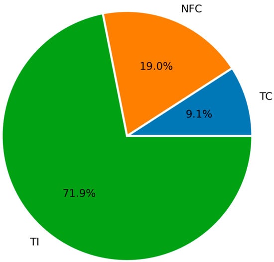
Figure 4. Distribution of the thermodynamic consistency test results for the N₂O + IL systems using the Peng–Robinson and Kwak–Mansoori model (PR/KM).

3.2. Prediction Using Multilayer Perceptron

All available experimental data were incorporated in the ANN training stage, including those previously identified as thermodynamically inconsistent. In this study, the ANN toolbox available in MATLAB 2025a [41] is used to implement a multilayer perceptron (MLP) composed of one input layer, two hidden layers, and one output layer. The architectures are of the (l, m, n, 1) type, where m and n represent the number of neurons in the hidden layer, and l = 4, 5, and 6 represent the combination of inputs. To bypass overfitting, we studied architectures with a maximum of 10 neurons per hidden layer such that n = 2, 3, … for the first hidden layer and m = 2, 4, 6, 8, and 10 for the second hidden layer.

The optimization of the model involves five steps: (i) select the initial model; (ii) optimize of the first hidden layer; (iii) optimize of the second hidden layer; (iv) evaluate of the different input combinations; and (v) evaluate the different learning algorithms. To reduce overfitting in the model, the data were randomly divided into three sets: 449 data points for training, 24 points for testing, and 24 points for prediction (the complete datasets are provided in the Supplementary Materials).

The criteria for selecting the best model were the average absolute deviation |Δx1%| and the maximum individual absolute deviation |Δx1%|_max (see Equations (10) and (11)). The above metrics are frequently used in the modeling of gas solubility in ILs [42,43]. This ensures that the ANN does not generate solubility predictions with negative values or values greater than one. Furthermore, we prioritized ANN architectures with a reduced number of parameters to achive a balance between accuracy and model simplicity. Previous studies on gas+IL systems have shown that choosing models with fewer parameters can minimize bias and variance without compromising accuracy [29,43,44]. The number of epochs for training the algorithms was set to 900, and each architecture is executed for 30 iterations. In addition, all the selected architectures were evaluated using testing and prediction datasets to verify their performance. Details of the calculation method are presented in the code used, which is available in the Supplementary Materials.

A simple model with four input variables of the form (4, m, 2, 1) is considered for optimizing of the first hidden layer. The input variables are the experimental temperature (T), experimental pressure (P), critical temperature (Tc), and critical pressure (Pc). Temperature and pressure are the common independent variables use to define thermodynamic properties, and the critical pressure and critical temperature are extensively used according to the corresponding state principle [37]. On the other hand, the Levenberg–Marquardt function is selected as the learning algorithm. This scheme has been shown to achieve an appropriate balance between convergence speed and overfitting control on medium-sized datasets [45,46]). The selection of both the variables and the algorithm is based on previous results reported in the literature.

The findings show that for m = 8 and 10, acceptable average absolute deviations were obtained. For the case (4, 8, 2, 1), the average absolute deviation is 4.37%, with a maximum individual absolute deviation of 46.57% during training. For the (4, 10, 2, 1) architecture, the average absolute deviation is 4.00%, and the maximum individual absolute deviation is 41.88% during training. Therefore, the (4, 10, n, 1) architecture is selected exhibiting the best performance in the training stage. The average absolute deviations in solubility for the entire set of m values considered in this study are shown in Figure 5.

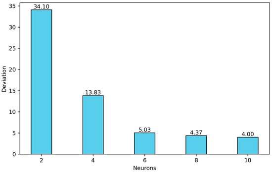
Figure 5. Optimization of the first hidden layer for architectures of type (4, m, 2, 1) with m = 2, 4, 6, 8 and 10.

In the optimization of the second hidden layer, combinations of neurons in the hidden layers with m = 4 and n = 2, 4, 6, 8, and 10 were analyzed. Table 5 presents the runs with the lowest average absolute deviation during the training, testing, and prediction stages for each architecture. In general, acceptable prediction results were found for the different architectures studied. Nevertheless, the (4, 10, 8, 1) architecture with 147 parameters stands out for exhibiting average absolute deviations below 3.50% for the three datasets and achieving the lowest |Δx₁%|_max = 7.56% in prediction.

Table 5. Results of the (4, 10, n, 1) using four input combinations T, P, Tc, and Pc, and the Levenberg Marquard algorithm (Np: parameter number).

Input	Architecture	Np	Run	Training (449 Data Point)		Testing (24 Data Point)		Prediction (24 Data Point)
				|Δx1%|	|Δx1%|max	|Δx1%|	|Δx1%|max	|Δx1%|	|Δx1%|max
T, P, Tc, and Pc	4, 10, 2, 1	75	14	4.00	41.88	7.17	60.06	2.48	9.55
	4, 10, 4, 1	99	30	3.43	48.92	3.97	13.34	3.03	13.04
	4, 10, 6, 1	123	05	2.21	26.36	3.15	11.31	2.98	11.07
	4, 10, 8, 1	147	01	1.86	18.97	3.48	15.74	1.81	7.56
	4, 10, 10, 1	171	03	1.95	37.49	2.98	15.80	2.84	13.09

The correlation between the experimental and calculated solubilities for the (4, 10, 8, 1) model and the T-P-Tc-Pc combinations is shown in Figure 6. The Pearson correlation coefficient was 0.9998 for the training set, 0.9992 for the testing set, and 0.9986 for the prediction set. In addition, the largest relative deviation is found in the low-solubility system (Figure 7). This is reasonable because of to the experimental uncertainty inherent in these measurements.

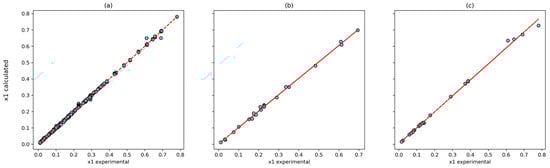
Figure 6. Correlation between experimental data and calculated by ANN using T, P, Tc and Pc inputs with (4, 10, 8, 1) architecture: (a) training dataset; (b) testing dataset; and (c) prediction dataset.

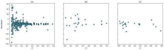
Figure 7. Dispertion between experimental data an calculated by ANN using T, P, Tc, and Pc inputs with (4, 10, 8, 1) architecture: (a) training dataset; (b) testing dataset; and (c) prediction dataset.

We also evaluated two alternative input sets: T-P-Tc-Pc-ω and T-P-Tc-Pc-Zc. When the acentric factor ω is added as a training variable, an increase in the average absolute deviation is observed in all datasets with the (5, 10, n, 1) architecture. For example, the (5, 10, 10, 1) architecture with 181 parameters results in the lowest maximum individual absolute deviation; however, the average absolute deviation increases for all three datasets compared with that of the (4, 10, 8, 1) architecture. A similar situation occurs when the critical compressibility factor and acentric factor are incorporated. In this case, for architectures of the type (6, 10, n, 1), the model achieves average absolute deviations of less than 10% in prediction. In particular, the (6, 10, 8, 1) architecture with 167 parameters can be identified as an acceptable model, with average absolute deviations of 1.80% in the training stage, 3.57% in the testing stage, and 2.57% in the prediction stage. The results obtained for the different architectures studied are presented in Table 6.

Table 6. Results using two input combinations (T, P, Tc, Pc, and ω; and T, P, Tc, Pc, ω, and Zc) and the Levenberg Marquard algorithm (Np: parameter number).

Input	Architecture	Np	Run	Training (449 Data Point)		Testing (24 Data Point)		Prediction (24 Data Point)
				|Δx1%|	|Δx1%|max	|Δx1%|	|Δx1%|max	|Δx1%|	|Δx1%|max
T, P, Tc, Pc and ω	5, 10, 2, 1	85	27	5.46	80.40	6.25	30.77	5.28	16.50
	5, 10, 4, 1	109	03	2.60	33.69	3.93	17.47	2.86	13.04
	5, 10, 6, 1	133	13	2.32	34.76	2.73	9.95	3.57	13.32
	5, 10, 8, 2	157	07	1.91	25.60	5.25	36.36	2.52	11.56
	5, 10, 10, 2	181	18	2.03	18.27	3.67	14.80	2.56	9.71
T, P, Tc, Pc, ω and Zc	6, 10, 2, 1	95	21	3.52	37.50	5.34	33.81	3.36	11.19
	6, 10, 4, 1	119	09	2.37	34.16	3.27	12.94	4.22	17.13
	6, 10, 6, 1	143	16	1.94	21.12	3.42	16.34	2.95	12.13
	6, 10, 8, 1	167	19	1.80	20.90	3.57	14.28	2.57	10.77
	6, 10, 10, 1	191	03	1.73	17.55	3.74	15.63	2.89	11.32

On the basis of these results, it is possible to select the variables T, P, Tc, and Pc as the input combination and the (4, 10, 8, 1) architecture as the best model for predicting the solubility of N₂O + ILs systems. The model is simple and has an acceptable number of parameters (147). It allows for the prediction of solubility for different temperature and pressure values with absolute deviations less than 10%. Experimental solubility measurements typically have uncertainties in the range of 5–10%. Therefore, the maximum deviation of 7.56% obtained is within the expected experimental variability in solubility models. In the case where an IL has not been considered for the training stage, it is only necessary to know its critical properties (Tc and Pc) and to incorporate them into the dataset to predict the solubility of new systems by using the model proposed in this work [29,43,44].

To complement this study, we evaluated seven additional learning algorithms using the (4, 10, 8, 1) architecture with the input variables T, P, Tc, and Pc. The results show that the algorithms with the lowest average absolute deviations are scaled conjugate-gradient (4.70%), BFGS quasi-Newton (5.14%), and Polak–Ribiére conjugate gradient (5.29%). Nevertheless, the Levenberg–Marquardt algorithm achieved the lowest average absolute deviation in the training, testing, and prediction stages. The average absolute deviations obtained for each learning algorithm considered in this work are shown in Figure 8.

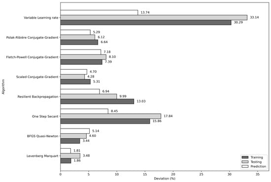
Figure 8. Average absolute deviations of the eight algorithms used in the training of the (4, 10, 8, 1) architecture and T, P, Tc, and Pc input combination.

The results obtained show that the MLP model can predict solubility with good accuracy, even when 71.9% of the dataset has been declared thermodynamically inconsistent. This shows that ANNs have sufficient flexibility to absorb noise or data dispersion that is declared thermodynamically inconsistent. It is important to clarify that when a dataset is thermodynamically inconsistent, this does not necessarily mean that the data are wrong. In such cases, correlating the data with an ANN simply demonstrates that the ANN model is capable of representing the dataset in much the same way that equations of state are used to model data for pure components and mixtures. This predictive capacity can be explained by the ability of MLP to learn the implicit patterns present in the overall dataset. Thermodynamic modeling is limited by data segmentation and by the requirement of internal coherence within each subset. For example, the PR/KM model correlates solubility at a fixed temperature (T) by fitting interaction parameters (k_ij, l_ij, m_ij) that are valid only for that specific P-T-x dataset. In contrast, the MLP model simultaneously integrates the characteristics of the complete dataset, thereby capturing nontrivial relationships between temperature, pressure, and solubility. Sufficiently large datasets can enable the network to learn the dominant underlying patterns despite local thermodynamics inconsistencies. The objective of ANN is to minimize error by capturing global trends that describe the average physical behavior of the system, without restricting itself to satisfying exact point-to-point relationships, as is the case with classical methods based on equations of state. These results indicate that the MLP model-based approach is a robust and flexible alternative, even when heterogeneous databases or those partially declared thermodynamically inconsistent are used.

In future work, other machine learning models—such as support vector machines (SVM) and random forest regressors (RFR)—will be evaluated to study the effect of thermodynamically inconsistent data on solubility prediction. In addition, the use of physics-informed neural networks (PINNs) will be explored to incorporate fundamental thermodynamic relationships—such as the Gibbs–Duhem equation and the corresponding states principle—directly into the neural network learning process.

4. Conclusions

In this work, the solubility of N₂O in various ionic liquids was modeled using a multilayer perceptron (MLP) artificial neural network. A total of 498 experimental data points were analyzed using a thermodynamic consistency test based on the Gibbs–Duhem equation and the Peng–Robinson equation of state with the Kwak–Mansoori mixing rule (PR/KM). The test results revealed that only 9.1% of the data were thermodynamically consistent (TC), 19.0% were not fully consistent (NFC), and 71.9% were classified as thermodynamically inconsistent (TI). Despite the high proportion of thermodynamically inconsistent data, the MLP model demonstrated a remarkable ability to predict N₂O solubility with high accuracy. The optimal architecture (4, 10, 8, 1), using temperature, pressure, and critical properties (T, P, Tc, Pc) as inputs and the Levenberg–Marquardt training algorithm, achieved an average absolute deviation of 1.81% and a maximum individual deviation of 7.56% in the prediction set. The comparative analysis of eight learning algorithms confirmed the superiority of the Levenberg–Marquardt algorithm, which produced significantly lower deviations (1.81%) compared to other methods. These findings suggest that MLPs can effectively capture underlying patterns in the experimental data, overcoming limitations associated with traditional thermodynamic modeling, which requires strict consistency within each isotherm. The (4, 10, 8, 1) architecture with 147 parameters represents the optimal balance between predictive accuracy and computational complexity.

References

- Radim, M.; de Loos, T.W.; Vlugt, T.H.J. State-of the-Art of CO2 Capture with Ionic Liquids. Ind. Eng. Chesmistry Res. 2012, 51, 8149–8177. [Google Scholar]
- Chen, Y.; Mutelet, F.; Jaubert, J.-N. Solubility of carbon dioxide, nitrous oxide and methane in ionic liquids at pressures close to atmospheric. Fluid Phase Equilibria 2014, 372, 26–33. [Google Scholar] [CrossRef]
- Román, Á.F.G.; Kabir, G. Assessing carbon dioxide emissions in manufacturing industries: A systematic review. Energies 2024, 17, 5119. [Google Scholar] [CrossRef]
- Lin, T.Y.; Chiu, Y.H.; Chen, C.H.; Ji, L. Renewable energy consumption efficiency, greenhouse gas emission efficiency, and climate change in Europe. Geoenergy Sci. Eng. 2025, 247, 213665. [Google Scholar] [CrossRef]
- Ramanathan, V. Trace Gas Greenhouse Effect and Global Warming, Underlying Principles and Outstanding Issues. Ambio 1998, 27, 187–197. [Google Scholar]
- Davidson, E.A. The contribution of manure and fertilizer nitrogen to atmospheric nitrous oxide since 1860. Nat. Geosci. 2009, 2, 659–662. [Google Scholar] [CrossRef]
- Tian, H.Q.; Xu, R.T.; Canadell, J.G.; Thompson, R.L.; Winiwarter, W.; Suntharalingam, P.; Davidson, E.A.; Ciais, P.; Jackson, R.B.; Janssens-Maenhout, G.; et al. A comprehensive quantification of global nitrous oxide sources and sinks. Nature 2020, 586, 248–256. [Google Scholar] [CrossRef]
- Reimer, R.A.; Slaten, C.S.; Seapan, M.; Lower, M.W.; Tomlinson, P.E. Abatement of N2O emissions produced in the adipic acid industry. Environ. Prog. 1994, 13, 134–137. [Google Scholar] [CrossRef]
- Filonchyk, M.; Peterson, M.P.; Zhang, L.; Hurynovich, V.; He, Y. Greenhouse gases emissions and global climate change: Examining the influence of CO2, CH4, and N2O. Sci. Total Environ. 2024, 935, 173359. [Google Scholar] [CrossRef]
- Pérez-Ramírez, J.; Kapteijn, F.; Schöffel, K.; Moulijn, J.A. Formation and control of N2O in nitric acid production: Where do we stand today? Appl. Catal. B Environ. 2003, 44, 117–151. [Google Scholar]
- Zhang, X.; Zhang, X.; Dong, H.; Zhao, Z.; Zhang, S.; Huang, Y. Carbon capture with ionic liquids: Overview and progress. Energy Environ. Sci. 2012, 5, 6668–6681. [Google Scholar] [CrossRef]
- Langham, J.V.; O’Brien, R.A.; Davis, J.H., Jr.; West, K.N. Solubility of CO2 and N2O in an imidazolium-based lipidic ionic liquid. J. Phys. Chem. B 2016, 120, 10524–10530. [Google Scholar]
- Amar, M.N.; Ghriga, M.A.; Seghier, M.E.A.B.; Ouaer, H. Predicting solubility of nitrous oxide in ionic liquids using machine learning techniques and gene expression programming. J. Taiwan Inst. Chem. Eng. 2021, 128, 156–168. [Google Scholar] [CrossRef]
- Holbrey, J.D.; Seddon, K.R. Ionic liquids. Clean Prod. Process. 1999, 1, 223–236. [Google Scholar] [CrossRef]
- Lei, Z.; Chen, B.; Koo, Y.M.; MacFarlane, D.R. Introduction: Ionic liquids. Chem. Rev. 2017, 117, 6633–6635. [Google Scholar] [CrossRef]
- Greer, A.J.; Jacquemin, J.; Hardacre, C. Industrial applications of ionic liquids. Molecules 2020, 25, 5207. [Google Scholar] [CrossRef]
- Valderrama, J.O.; Reategui, A.; Sanga, W. Thermodynamic consistency test of vapor-liquid equilibrium data for mixtures containing ionic liquids. Ind. Eng. Chem. Res. 2008, 47, 8416–8422. [Google Scholar] [CrossRef]
- Zhou, T.; Gui, C.; Sun, L.; Hu, Y.; Lyu, H.; Wang, Z.; Song, Z.; Yu, G. Ionic Liquids for Carbon Capture. Chem. Rev. 2023, 123, 12170–12253. [Google Scholar]
- Jacquemin, J.; Costa Gomes, M.F.; Husson, P.; Majer, V. Solubility of carbon dioxide, ethane, methane, oxygen, nitrogen, hydrogen, argon, and carbon monoxide in 1-buthyl-3-methylimidazolium tetrafluoroborate between temperatures 283 K and 343 K and at pressures close to atmospheric. J. Chem. Thermodyn. 2006, 38, 490–502. [Google Scholar]
- Kurnia, K.A.; Mathewaran, P.; How, C.J.; Noh, M.H.; Kusumawati, Y. Solubility of methane in alkylpyridinium-based ionic liquids at temperatures between 298.15 and 343.15 K and pressures up to 4 MPa. J. Chem. Eng. Data 2020, 65, 4642–4648. [Google Scholar] [CrossRef]
- Yokozeki, A.; Shiflett, M.B. Separation of Carbon Dioxide and Sulfur Dioxide Gases Using Room-Temperature Ionic Liquid [hmim][Tf2N]. Energy Fuels 2009, 23, 4701–4708. [Google Scholar] [CrossRef]
- Shiflett, M.B.; Elliott, B.A.; Niehaus, A.M.S.; Yokozeki, A. Separation of N2O and CO2 using Room-Temperature Ionic Liquid [bmim][Ac]. Sep. Sci. Technol. 2012, 47, 411–421. [Google Scholar] [CrossRef]
- Shiflett, M.B.; Niehaus, A.M.S.; Elliott, B.A.; Yokozeki, A. Phase Behavior of N2O and CO2 in Room-Temperature Ionic Liquids [bmim][Tf2N], [bmim][BF4], [bmim][N(CN)2], [bmim][Ac], [eam][NO3], and [bmim][SCN]. Int. J. Thermophys. 2012, 33, 412–436. [Google Scholar]
- Revelli, A.-L.; Mutelet, F.; Jaubert, J.-N. Reducing of Nitrous Oxide Emissions Using Ionic Liquids. J. Phys. Chem. B 2010, 114, 8199–8206. [Google Scholar] [CrossRef]
- Shaahmadi, F.; Anbaz, M.A.; Bazooyar, B. Analysis of intelligent models in prediction nitrous oxide (N2O) solubility in ionic liquids (ILs). J. Mol. Liq. 2017, 246, 48–57. [Google Scholar] [CrossRef]
- Feng, H.; Qin, W.; Hu, G.; Wang, H. Intelligent prediction of nitrous oxide capture in designable ionic liquids. Appl. Sci. 2023, 13, 6900. [Google Scholar] [CrossRef]
- Nakhaei-Kohani, R.; Atashrouz, S.; Hadavimoghaddam, F.; Bostani, A.; Hemmati-Sarapardeh, A.; Mohaddespour, A. Solubility of gaseous hydrocarbons in ionic liquids using equations of state and machine learning approaches. Sci. Rep. 2022, 12, 14276. [Google Scholar] [CrossRef]
- Mousavi, S.P.; Nakhaei-Kohani, R.; Atashrouz, S.; Hadavimoghaddam, F.; Abedi, A.; Hemmati-Sarapardeh, A.; Mohaddespour, A. Modeling of H2S solubility in ionic liquids: Comparison of white-box machine learning, deep learning and ensemble learning approaches. Sci. Rep. 2023, 13, 7946. [Google Scholar] [CrossRef]
- Faúndez, C.A.; Fierro, E.N.; Muñoz, A.S. Solubility of methane in ionic liquids for gas removal processes using a single multilayer perceptron model. Processes 2024, 12, 539. [Google Scholar] [CrossRef]
- Srinivasan, N.; Yang, S. Artificial neural network aided vapor–liquid equilibrium model for multi-component high-pressure transcritical flows with phase change. Phys. Fluids 2024, 36, 083328. [Google Scholar] [CrossRef]
- Bekri, S.; Özmen, D.; Özmen, A. Deep learning based combining rule for the estimation of vapor–liquid equilibrium. Braz. J. Chem. Eng. 2024, 41, 613–629. [Google Scholar] [CrossRef]
- Sun, J.; Xue, J.; Yang, G.; Li, J.; Zhang, W. Vapor–liquid phase equilibrium prediction for mixtures of binary systems using graph neural networks. AIChE J. 2025, 71, e18637. [Google Scholar]
- Bishop, C.M. Neural Networks for Pattern Recognition; Oxford University Press: Oxford, UK, 1995. [Google Scholar]
- Valderrama, J.O.; Faúndez, C.A.; Campusano, R. An overview of a thermodynamic consistency test of phase equilibrium data. Application of the versatile VPT equation of state to check data of mixtures containing a gas solute and an ionic liquid solvent. J. Chem. Thermodyn. 2019, 131, 122–132. [Google Scholar] [CrossRef]
- Valderrama, J.O.; Álvarez, V.H. A versatile thermodynamic consistency test for incomplete phase equilibrium data of high-pressure gas–liquid mixtures. Fluid Phase Equilibria 2004, 226, 149–159. [Google Scholar] [CrossRef]
- Valderrama, J.O.; Álvarez, V.H. Vapor–liquid equilibrium in mixtures containing supercritical CO2 using a new modified Kwak–Mansoori mixing rule. AIChE J. 2004, 50, 480–488. [Google Scholar]
- Prausnitz, J.M.; Lichtenthaler, R.N.; De Azevedo, E.G. Molecular Thermodynamics of Fluid-Phase Equilibria; Pearson Education: London, UK, 1999; Volume 3, pp. 245–247. [Google Scholar]
- Peng, D.Y.; Robinson, D.B. A new two-constant equation of state. Ind. Eng. Chem. Fundam. 1976, 15, 59–64. [Google Scholar] [CrossRef]
- Kwak, T.I.; Mansoori, G.A. Van der Waals mixing rules for cubic equations of state. Applications for supercritical fluid extraction modeling. Chem. Eng. Sci. 1986, 41, 1303–1309. [Google Scholar] [CrossRef]
- Valderrama, J.O.; Forero, L.A.; Rojas, R.E. A generalized form of the Kiselev equation for propane and carbon dioxide adsorption on activated carbons and activated carbon cloths. Ind. Eng. Chem. Res. 2015, 54, 3480–3487. [Google Scholar] [CrossRef]
- The MathWorks Inc. Matlab. 2025. Available online: https://www.mathworks.com/help/matlab/ (accessed on 11 June 2025).
- Shiflett, M.B.; Yokozeki, A. The solubility of gases in ionic liquids. AIChE J. 2017, 63, 4722–4737. [Google Scholar] [CrossRef]
- Fierro, E.N.; Faúndez, C.A.; Muñoz, A.S.; Cerda, P.I. Application of a single multilayer perceptron model to predict the solubility of CO2 in different ionic liquids for gas removal processes. Processes 2022, 10, 1686. [Google Scholar] [CrossRef]
- Fierro, E.N.; Faúndez, C.A.; Muñoz, A.S. Influence of thermodynamically inconsistent data on modeling the solubilities of refrigerants in ionic liquids using an artificial neural network. J. Mol. Liq. 2021, 337, 116417. [Google Scholar] [CrossRef]
- Hagan, M.T.; Menhaj, M.B. Training feedforward networks with the Marquardt algorithm. IEEE Trans. Neural Netw. 1994, 5, 989–993. [Google Scholar] [CrossRef] [PubMed]
- Song, Z.; Shi, H.; Zhang, X.; Zhou, T. Prediction of CO2 solubility in ionic liquids using machine learning methods. Chem. Eng. Sci. 2020, 217, 115752. [Google Scholar] [CrossRef]
Disclaimer/Publisher’s Note: The statements, opinions and data contained in all publications are solely those of the individual author(s) and contributor(s) and not of MDPI and/or the editor(s). MDPI and/or the editor(s) disclaim responsibility for any injury to people or property resulting from any ideas, methods, instructions or products referred to in the content. |
© 2025 by the authors. Licensee MDPI, Basel, Switzerland. This article is an open access article distributed under the terms and conditions of the Creative Commons Attribution (CC BY) license (https://creativecommons.org/licenses/by/4.0/).