Abstract
The operational modes and fault characteristics of distribution networks incorporating distributed generation are becoming increasingly complex. This complexity increases the difficulty of predicting switch control action times and leads to scattered samples with data scarcity. Consequently, it imposes higher demands on rapid fault isolation and load transfer control following system failures. To address this issue, this paper proposes a switch action time prediction and synchronous load transfer control method based on Bayesian optimization of bidirectional long short-term memory (Bo-BiLSTM) networks. A distribution network simulation model incorporating distributed generation was constructed using MATLAB/Simulink (R2023a). Three-phase voltage and current at the Point of Common Coupling (PCC) were extracted as feature parameters to establish a switch operation timing database. Bayesian optimization was employed to tune the BiLSTM hyperparameters, constructing the Bo-BiLSTM prediction model to achieve high-precision forecasting of switch operation times under fault conditions. Subsequently, a load-synchronized transfer control strategy was proposed based on the prediction results. A dynamic delay mechanism was designed to achieve “open first and then close” sequential coordinated control. Physical experiments verified that the time difference between opening and closing was controlled within 2–12 milliseconds (ms), meeting the engineering requirement of less than 20 ms. The results demonstrate that the proposed control method enhances switch operation time prediction accuracy while effectively supporting rapid fault isolation and seamless load transfer in distribution networks, thereby improving system reliability and control precision.
1. Introduction
With the large-scale integration of distributed generation (DG) into distribution networks, system operation modes and fault characteristics have become increasingly complex, placing higher demands on rapid fault isolation and load transfer control post-fault [1]. As the core component enabling distribution network automation and fault self-healing, the precise prediction of switching equipment response times is crucial for ensuring reliable operation of protection and control systems and minimizing outage duration [2]. However, DG integration significantly alters fault current magnitude and direction, resulting in highly dispersed and uncertain switch operation time samples. Concurrently, the scarcity of training data for predictive models is exacerbated by the challenges in collecting real-world fault data. These factors cause a significant decline in the accuracy of prediction methods based on traditional mechanism models or shallow learning algorithms, making it difficult to meet the stringent requirements for real-time control and reliability in smart distribution grids.
In recent years, deep learning techniques have achieved remarkable success in the field of time-series data forecasting. Long short-term memory (LSTM) networks and their variants have been widely applied in areas such as remaining equipment life prediction [3,4] and power load forecasting due to their exceptional ability to capture long-term sequential dependencies. However, standard LSTM models suffer from blindness in hyperparameter selection and predominantly employ unidirectional encoding, making it difficult to fully exploit the bidirectional contextual information inherent in time-series data. Although bidirectional long short-term memory (BiLSTM) networks enhance feature extraction through bidirectional encoding, their performance remains heavily dependent on optimized hyperparameter configurations [5]. Bayesian optimization (BO), as an efficient global hyperparameter optimization framework, can adaptively search for optimal hyperparameter combinations of complex models with minimal evaluation iterations, significantly improving model convergence speed and prediction accuracy [6].
Recent research has significantly advanced the application of complex artificial intelligence models in power systems. For instance, Reference [7] successfully integrated convolutional neural networks (CNNs) with bidirectional long short-term memory (BiLSTM) networks for equipment remaining life prediction, while Reference [8] employed Bayesian optimization of long short-term memory (LSTM) networks for distribution system state estimation. Concurrently, studies such as [9] focus on enhancing fault classification accuracy through hybrid deep learning models. Collectively, these achievements confirm a clear trend: integrating advanced neural networks with intelligent optimization has become a key research paradigm for enhancing the perception and predictive capabilities of power systems.
While previous studies have explored LSTM and BiLSTM networks for fault diagnosis and switch time prediction and Bayesian methods for model optimization [10], a significant gap remains. Existing work primarily focuses on improving prediction accuracy alone, often overlooking the critical next step: the seamless integration of these high-fidelity predictions into a real-time, reliable control strategy for load transfer. The challenge of closing the loop from “accurate prediction” to “precise control” in a single framework, especially under the constraints of small sample sizes and high data dispersion, has not been fully addressed.
Based on this, this paper addresses the challenge of high-precision prediction of switch operation times in distribution networks under DG integration and further applies the prediction results to the precise control of synchronous load transfer. The main contributions of this study are as follows:
- A Bo-BiLSTM-based prediction model for switching operation timing in distribution networks is proposed. By adaptively obtaining optimal hyperparameters for the BiLSTM network through Bayesian optimization algorithms, the model’s predictive accuracy and generalization capability are effectively enhanced under conditions of small sample sizes and high data dispersion, laying the foundation for subsequent implementation of control strategies.
- A comprehensive database of switch operation time characteristics was established. A detailed simulation model of the distribution network incorporating DG was constructed using MATLAB/Simulink. This model simulated 620 operational scenarios encompassing various short-circuit fault types, different fault locations, and transition resistances, providing a robust data foundation for model training and control logic validation.
- We innovatively integrate switch timing prediction results with load transfer control strategies. Based on the predicted time parameters, a synchronous transfer control strategy was designed following the principle of “open first and then close” with dynamic delay, Δt, as its core. Physical experiments validated that this strategy can strictly control the opening and closing time difference within a 20 ms safety margin, with experimental results ranging from 2 to 12 ms. This fundamentally eliminates the risk of circulating currents caused by asynchronous closing, achieving seamless load transfer control after a fault.
This study not only provides a novel data-driven solution for predicting switching control action time in distribution networks but also establishes a comprehensive technical framework spanning from “precise prediction” to “precise control.” It holds significant theoretical value and engineering significance for enhancing the power supply reliability and self-healing control capabilities of distribution networks under high-penetration DG access.
Figure 1 illustrates the overall workflow of this study, which forms a closed loop from data-driven prediction and model optimization to control strategy and experimental validation.
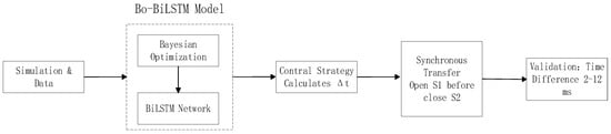
Figure 1.
Schematic diagram of the research framework.
2. System Modeling and Feature Database Construction
2.1. System Modeling
This paper investigates the switching sequence of distribution network switches during different feeder faults in a distribution system with a distributed photovoltaic (PV) connection to a double-feeder network. A typical distribution network model incorporating a distributed PV system is constructed, featuring a 35 kV system voltage, one distributed PV generator, and L1 and L2, representing loads. The structure is illustrated in Figure 2.
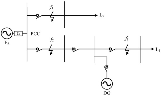
Figure 2.
Topology diagram for distributed PV integration into distribution networks.
By continuously monitoring and analyzing parameters such as current and voltage at the Point of Common Coupling (PCC), various faults occurring in the distribution system can be promptly detected and addressed, ensuring reliable power supply. The operational conditions of the grid and the specific fault type determine the switching action time [11].
This paper selects fault types, locations, and transition resistance values based on power system engineering principles and distribution network fault scenarios. Fault types include single-phase grounding, two-phase short circuit, two-phase grounding short circuit, and three-phase short circuit. Fault locations are chosen at the feeder head, midpoint, and feeder tail. The study evaluates the impact of fault point distance from the power source and distributed power sources on protection system operation and switching sequence timing, covering scenarios with varying contributions from main grid and distributed power source fault currents. The grounding transition resistance values range from 0.001 Ω to 130 Ω, testing the model’s sensitivity and accuracy under various fault conditions. Key system equipment and model parameters are listed in Table 1.

Table 1.
Table of system parameters.
This paper established a distribution network system simulation model using MATLAB/Simulink. It obtained voltage and current conditions at the Point of Common Coupling (PCC) during different types of faults occurring at frequencies f1, f2, and f3. Subsequently, it recorded and analyzed the switching operation times of distribution network switches from both voltage and current perspectives after integrating distributed power sources into the distribution network. This provided historical data support for subsequent predictive control.
2.2. Construction of a Database for Time Characteristics of Distribution Network Switch Operations
Distribution networks can be broadly categorized into 12 operational conditions: single-phase short circuits (AG, BG, CG), two-phase short circuits (AB, AC, BC), two-phase grounded short circuits (ABG, ACG, BCG), three-phase short circuits (ABC), three-phase grounded short circuits (ABCG), and non-fault states. Simulations were conducted for different distribution network conditions, collecting three-phase voltage and current data at the PCC for each scenario to construct a database of switch operation time characteristics for the distribution network. In power system transient analysis, voltage and current peaks serve as the most direct and stable key physical quantities characterizing abrupt system state changes. Therefore, these peak values were employed as inputs for the credibility network classifier, as shown in Table 2.
Table 2.
Time-characteristic parameters of grid switch operation.
The peak voltage and peak current values in Table 2 were calculated based on simulation sampling data. This study obtained 620 operating conditions through simulation, denoted as O1–O620. The six characteristic data points and switching action times under different operating conditions are shown in Appendix A, Table A1.
To eliminate the influence of feature dimensions and enhance model training stability, this study employs the Z-Score normalization method to process the feature matrix. This approach transforms each feature column into a distribution with a mean of 0 and a standard deviation of 1, enabling comparability among different features while preserving the distribution characteristics of the original data. It is suitable for subsequent gradient-optimized deep learning models. Taking O1 as an example, its normalization process follows the method below:
In the formula, Vi and Vi′ denote the normalized and pre-normalized values of the i-th operational state symptom attribute, respectively; μ denotes the mean of each feature column across all samples; and σ denotes the standard deviation, calculated for S2 through S620. The normalized database is shown in Appendix A, Table A2.
The normalization of the feature matrix involves six operational status indicators for each operating condition in the database, collectively forming a feature vector. A training dataset comprising 620 × 70% = 434 feature vectors is randomly selected from the database, while the remaining 620 × 30% = 186 vectors serve as the test dataset.
3. Bayesian Optimization-Based BiLSTM Forecasting Model
3.1. BiLSTM Principles and Applicability
The LSTM algorithm is used to process and predict highly time-dependent, strongly coupled events, but LSTM network models exhibit lower adaptability [12,13]. Unlike LSTM networks, BiLSTM consists of two independent forward and backward LSTM networks, one for forward propagation and the other for backward propagation. In each time step, the forward LSTM processes the input sequence in forward order, while the backward LSTM processes it in reverse order. This allows each LSTM unit to simultaneously access both preceding and subsequent contextual information. Furthermore, compared to other methods—such as random forests and gradient boosters, which are powerful for tabular data but primarily model static correlations—BiLSTM inherently incorporates temporal state mechanisms [14]. These mechanisms are crucial for simulating causal, time-dependent processes from fault states to protective actions. Similarly, purely unsupervised learning approaches are unsuitable for regression-based prediction tasks. Standard recurrent neural networks encounter gradient vanishing issues when capturing long-range dependencies. The LSTM architecture and its gating mechanism were specifically developed to overcome this limitation, making it a superior choice for learning the potentially long and complex causal pathways inherent in power system fault responses. Therefore, BiLSTM was selected to most effectively capture the rich temporal dependencies present in the data [15].
This study employed BiLSTM to capture the temporal characteristics of electrical quantities before and after failures, performing bidirectional training on sample failure data. The schematic diagram of the BiLSTM structure is shown in Figure 3 [16].
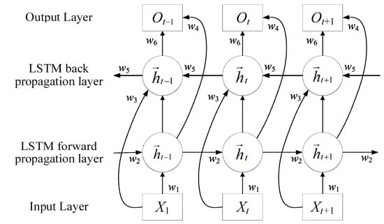
Figure 3.
BiLSTM architecture diagram.
3.2. Bayesian Optimization Principle
Bayesian optimization employs Gaussian processes as probabilistic surrogate models, enhancing algorithmic robustness through continuous iteration on existing sample data [17]. When determining new prediction points, Bayesian algorithms require maximizing the utility function. Thus, while not applicable to every optimization problem, Bayesian algorithms constitute an effective global optimization approach. Bayesian optimization comprises Gaussian process regression and acquisition function computation. Gaussian process regression yields the mean and variance of the function value, while the acquisition function constructs a sampling strategy based on these parameters to determine the sampling points for the current iteration.
- (1)
- Gaussian Process Regression
Gaussian process regression (GPR) is a nonparametric Bayesian method for solving regression problems [18]. GPR is based on a Gaussian process prior distribution, which is adjusted by observational data to yield a posterior distribution [19]. Its model assumptions comprise both noise and Gaussian process prior components, with solutions derived through Bayesian inference.
- (2)
- Collection Function
The sampling function generates the next observation point to be predicted. Based on the mean and covariance dataset D calculated by Gaussian process regression, it determines the next sample point after iteration. Its primary role is to accelerate convergence by leveraging previous observations while simultaneously exploring regions of high uncertainty within the decision space, thereby avoiding getting stuck in local optima.
The Bayesian optimization process is meticulously configured to ensure efficient and reproducible hyperparameter search. The search targets four key BiLSTM hyperparameters within the following ranges: the number of hidden units is optimized as an integer between 32 and 128; the initial learning rate is searched on a logarithmic scale between 1 × 10⁻⁴ and 1 × 10⁻²; the L2 regularization factor is explored on a logarithmic scale between 1 × 10⁻⁵ and 1 × 10⁻²; and the gradient threshold is adjusted within [0.5, 2] to prevent gradient explosion. A Gaussian process with a Matern 5/2 kernel was selected as the surrogate model for its flexibility in capturing diverse function behaviors. Optimization is guided by an expectation-maximization (EM) sampling function to effectively balance exploration and exploitation. The process is capped at 50 iterations, representing a trade-off between computational cost and performance. Convergence is assessed by monitoring the relative improvement in the optimal observation target value; the search is deemed converged if this improvement falls below a 0.2% tolerance for ten consecutive iterations.
3.3. Bo-BiLSTM Network Parameter Optimization
The hyperparameters of BiLSTM are difficult to set manually, so a Bayesian optimization (BO) approach is employed to automatically identify the optimal hyperparameter combination, aiming to achieve higher prediction accuracy. Given the large number of parameters in the BiLSTM network, the BO algorithm is used to optimize several key parameters within the network. This ensures that the optimized parameters achieve the best possible fit with the network, enabling high-precision data prediction.
The hyperparameter selection formula for Bayesian optimization is as follows:
In the formula, f(x) denotes the optimization function; x represents the set of optimization parameters; X is the set of optimization parameter sets; and x* is a set of optimization functions.
Define the Error function as the prediction error rate function for the BiLSTM model, with the formula as follows:
In the formula, N represents the total number of sample groups; R denotes the number of sample groups in N where the predicted values match the actual loss values.
The BiLSTM weight update formula is
In the formula, α denotes the learning rate; n represents the mini-batch size. It can be seen from the formula that α and n influence the weight updates of the network, with α affecting the step size per iteration and n determining the network’s loss function.
3.4. Switch Operation Time Prediction Method for Distribution Networks Based on Bo-BiLSTM Network
The modeling and testing process of the Bo-BiLSTM network is illustrated in Figure 4. First, switch test data from distribution network simulations is acquired, smoothed, and divided into training and test sets. Next, the Bo algorithm is applied to tune hyperparameters on the training set, with the optimal settings fed back to reconstruct the BiLSTM network. Finally, predictions are made on the test set data.
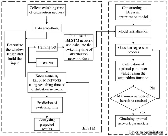
Figure 4.
Bo-BiLSTM prediction model workflow.
The optimization process of the model can be divided into the following steps.
- (1)
- Model initialization: Define the function f(x) and the definition domain of x to be optimized in the Bayesian optimization algorithm, set the objective function and the maximum number of iterations, etc.; divide the processed failure characteristics dataset into test set kernel and training set; and train the BiLSTM model.
- (2)
- Select the BiLSTM model failure prediction error rate to obtain the initial observation of the Bayesian algorithm.
- (3)
- The Gaussian process is applied to estimate the initial observation value to determine the next observation point.
- (4)
- Select the optimal parameters according to the acquisition function until the end of the iteration.
- (5)
- The optimal parameters obtained by the Bayesian algorithm are brought into the BiLSTM network for parameter reconstruction.
- (6)
- The optimal parameters are brought into the BiLSTM model to predict the test set data, and the predicted results are obtained and analyzed.
4. Analysis of BiLSTM Prediction Model Results
4.1. Model Prediction Standard
The goodness-of-fit coefficient (R2), root mean square error (RMSE), and mean absolute error (MAE) can be used to evaluate the performance of time-series forecasting algorithms. R2 indicates the degree of fit between the data and the regression model; the RMSE represents the average value of errors, reflecting the model’s stability; and the MAE accurately reflects the magnitude of actual prediction errors. Their expressions are as follows:
In the formula, xtri is the true value, is the average of the true value, xpri is the predicted value, and N is the number of predictions.
4.2. Bayesian Optimization Search Results
The Bayesian optimization algorithm repeatedly refines the target value through computational operations of the collection function. By continuously computing the objective function, it seeks the global optimum to optimize the BiLSTM network, ensuring more precise prediction results. The Bayesian optimization results are shown in Figure 5.
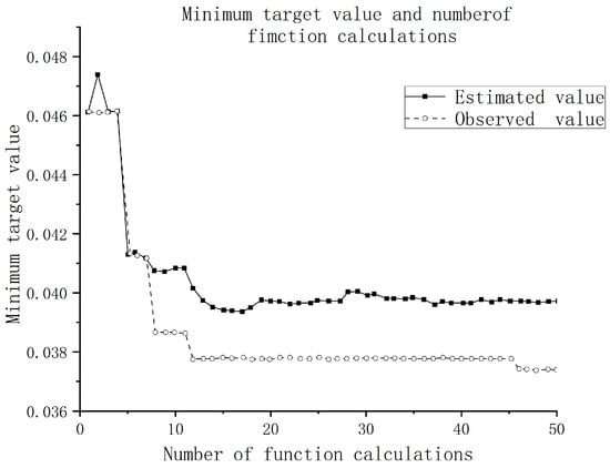
Figure 5.
Bayesian optimization.
Figure 5 illustrates the convergence characteristics of the Bayesian optimization algorithm during the hyperparameter auto-tuning process, reflecting the iterative trajectory of hyperparameter tuning within the constructed Bo-BiLSTM prediction model. The horizontal axis represents the number of function evaluations, while the vertical axis shows the minimum objective value. The figure also compares the algorithm’s estimated values of the objective function with the actual observed values throughout the iteration process. As iterations increase to the preset 50, the two curves gradually converge and eventually stabilize. After 50 function evaluations, the minimum objective value decreases from an initial value of approximately 0.048 to 0.0378. This value falls within a tolerance of less than 0.2% compared to the estimated minimum objective value of 0.0395, indicating that the search has converged.
To clearly present the final model structure determined through Bayesian optimization, Table 3 lists the core hyperparameters of the BiLSTM network and their optimal values. This set of parameters was automatically identified by the Bayesian optimization algorithm through 50 iterative evaluations within a predefined search space, directly corresponding to the configuration where the objective function converged to its minimum value, as shown in Figure 5.
Table 3.
The optimal hyperparameter set for the BiLSTM network obtained through Bayesian optimization.
Specifically, the optimized number of hidden units was set to 96, achieving a balance between model capacity and computational efficiency; the initial learning rate was 3.16 × 10⁻³, facilitating a stable descent of the “adam” optimizer during early training. The L2 regularization coefficient was set to 2.45 × 10⁻⁴ to effectively suppress overfitting without excessively compromising fitting capability; the gradient threshold was set to 1.2 to prevent gradient explosion during training. This set of parameters collectively formed the final architecture of the Bo-BiLSTM network used for switch timing prediction, serving as the performance foundation for achieving high-accuracy predictions.
4.3. Distribution Network Switching Time Prediction Results
To evaluate the performance of the proposed Bo-BiLSTM model, we employed a widely recognized robust benchmark—Extreme Gradient Boosting (XGBoost). As an efficient and practical implementation of gradient boosting algorithms, XGBoost has consistently achieved top results in numerous machine learning competitions and structured data regression tasks, establishing itself as a powerful non-deep learning benchmark. The hyperparameters of the XGBoost model—including the learning rate, maximum tree depth, and number of estimators—were optimized using the same Bayesian optimization framework as that in BiLSTM to ensure a fair and rigorous comparison. The models were trained and tested on the same datasets described in Section 2.2.
The first 70% of the distribution network switch time series was used as the training set, while the remaining 30% served as the test set. The delay step size was set to 15, the solver was configured as “adam”, and the initial learning rate was 0.005. Training was conducted for 250 epochs with a learning rate decay factor of 0.2 and a decay cycle of 125. To prevent gradient explosion, the gradient threshold was set to 1.
The prediction results of the three network models for distribution network switching times are shown in Figure 6.
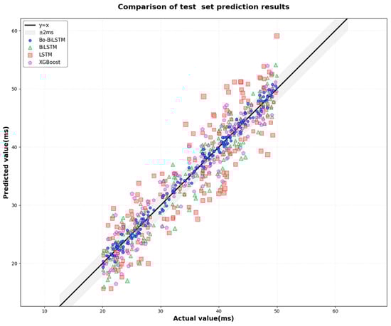
Figure 6.
Comparison of prediction results from different network models on the test set.
This figure compares the prediction results of four different network models against actual simulation data on the same test set. Visual verification via the coordinate axes clearly shows that the Bo-BiLSTM model’s prediction curve most closely aligns with actual values, demonstrating the highest consistency and stability. The BiLSTM and LSTM models follow in performance, while XGBoost exhibits noticeable deviations under certain operating conditions. This indicates that the fusion architecture integrating the attention mechanism (Bo) with the bidirectional long short-term memory network (BiLSTM) effectively enhances the ability to capture complex time-series fault features and improves prediction accuracy.
The performance of the prediction models is quantitatively evaluated using three standard metrics: R2, the RMSE, and the MAE. A superior model is characterized by an R2 value closer to 1, indicating a better fit to data, while simultaneously achieving lower RMSE and MAE values, which reflect higher prediction accuracy and smaller error magnitudes. A comparison of these metrics for the Bo-BiLSTM, BiLSTM, LSTM, and XGBoost models is presented in Table 4.
Table 4.
Comparison of prediction metrics for distribution network switch operation time prediction models.
As shown in Table 4, for the prediction metrics of the distribution network switch operation time prediction model, the Bo-BiLSTM network achieved a model fit quality of 0.91464, representing improvements of 0.29476 and 0.36749 compared to the BiLSTM and LSTM networks, respectively. The root mean square error was 0.59996, representing reductions of 0.59004 and 0.702224 compared to the BiLSTM and LSTM networks, respectively. The mean absolute error was 0.49855, showing decreases of 0.52335 and 0.61455 relative to the BiLSTM and LSTM networks.
Bo-BiLSTM achieved approximately 11.34% higher R2 scores than XGBoost, while reducing the root mean square error (RMSE) and mean absolute error (MAE) by approximately 29.43% and 28.92%, respectively, demonstrating a significant competitive advantage. This performance gap highlights the key strengths of our proposed architecture.
To more intuitively demonstrate the superiority of the Bo-BiLSTM model in time prediction, the prediction error was calculated between the predicted and actual switch operation times for the 100th sample point in the distribution network. The prediction errors for switch operation times under different network models are shown in Table 5.
Table 5.
Bo-BiLSTM network model prediction error table.
The absolute error values for the four network models, as shown in the table, are 0.76186, 1.34878, 2.1639, and 1.67838, respectively. The Bo-BiLSTM network exhibits the smallest absolute error in its predictions, indicating superior predictive performance.
It should be noted that the validation of this study is primarily based on the constructed typical distribution network model and its derived dataset. Although the model’s effectiveness was demonstrated through training–test set partitioning and physical experiments, future work will include testing in distribution network cases with different topologies and higher penetration rates of distributed generation (DG) to further evaluate the model’s broad applicability.
4.4. Discussion on Prediction Error Accumulation
An observation from the prediction results is that the discrepancy between the actual and predicted values tends to increase with the sample point index along the testing timeline. This phenomenon, often referred to as error accumulation, is a known challenge in sequence-to-sequence prediction tasks and can be attributed to the following factors:
- Temporal Dependency and Autoregressive Nature: The BiLSTM model makes predictions based on a sequence of previous time steps. In an autoregressive setting, the current prediction relies on past observed or predicted values. As the prediction horizon extends into the future, the model increasingly depends on its own previous predictions rather than ground-truth data. Any small error made at an early step can therefore be propagated and amplified in subsequent predictions, leading to a gradual divergence from the actual series.
- Attenuation of Long-range Contextual Information: Although BiLSTM is designed to capture long-term dependencies, its ability to retain and utilize information from the distant past is still finite. For very long sequences or sequences with complex, non-stationary patterns, the influence of the initial, most informative states of the network may diminish over time. This makes it increasingly difficult for the model to correct its course based on the foundational context.
- Limitations of the Training Dataset: Our model was trained on a finite set of 620 operational scenarios. While this provides a solid foundation, the testing sequence might encounter a subtle, cumulative combination of features that represents an edge case or a gradual shift in system dynamics not fully captured in the training distribution. The model, having not been explicitly trained on such a prolonged, specific trajectory, struggles to maintain perfect accuracy.
It is important to note that despite this observed accumulation, the Bo-BiLSTM model demonstrated superior robustness compared to the baseline BiLSTM and LSTM models. As quantified in Table 4 and Table 5, the absolute magnitude of its errors remained significantly lower throughout the sequence. This indicates that the Bayesian optimization successfully found a parameter set that minimized the initial error and slowed the rate of accumulation, thereby enhancing the model’s practical utility for a sufficient prediction horizon relevant to the subsequent control action.
5. Time-Based Model and Experimental Validation for Full-Process Control of Load Transfer Using Bo-BiLSTM
Accurate switch timing prediction provides the prerequisite for achieving precise load transfer control.
This chapter will design a synchronous control strategy based on the switching times predicted by the Bo-BiLSTM model to ensure the safety and rapidity of the transfer process. The core control objective of the model is to accurately estimate the total time control interval from the issuance of the master station command to the final switching action, while ensuring compliance with the “open first and then close” sequence and time difference constraints even under extreme scenarios. By integrating mathematical modeling with engineering experience, we can systematically evaluate the boundary conditions of time parameters and their impact mechanisms on the overall control process, providing theoretical support for strategy design. This strategy requires, based on precise time synchronization, that the time interval from complete open ping to complete closing be within 20 ms, disregarding communication time from the master station to the terminal.
5.1. Time Constraints and Problem Modeling
Control Objective: The total time interval from the completion of the original power switch (S1) opening to the completion of the target power switch (S2) closing must satisfy the safety constraint:
0 < Ttotal < 20 ms
- Known Conditions:
Based on the Bo-BiLSTM model predictions, the closing operation time of the target switch S2 (T_close) is shorter than the opening operation time of the original switch S1 (T_open).
- Master Station Command Sequence:
To achieve the “open first and then close” logic and compensate for the time difference, the master station issues commands with a dynamic delay (Δt):
t0: Issue the closing command to the target switch (S2).
t0 + Δ: Issue the opening command to the original switch (S1).
- Mathematical Model:
Completion time of closing operation (S2):
Completion time of opening operation (S1):
The total time interval is defined as the period from the end of the opening to the end of the closing:
In the formula, the physical meaning of Ttotal is the time interval from the complete opening of the main contacts of the original power switch to the complete closing of the main contacts of the target power switch. This interval represents the duration during which the load side is actually deprived of power supply during the load transfer process.
The control objective can be formulated as the following constraint:
0 < Ttotal < 20 ms
5.2. Control Strategy Design: Determination of Dynamic Delay Time Δt
The core of the control strategy is to calculate the dynamic delay Δt such that Ttotal always falls within the safe range, even with prediction errors. Δt is a time offset precalculated by the master station and embedded within the control command. Its implementation does not depend on the interval between sequential commands issued by the master station but rather relies on high-precision distributed time synchronization.
Derivation of the Constraint for Δt:
From Equation (10) and the control objective 0 < Ttotal < 20 ms, we can derive the feasible range for Δt:
- For Ttotal > 0: T_close − T_open − Δt > 0 => Δt < T_close − T_open
This ensures that the opening operation completes before the closing operation, preventing paralleling.
- 2.
- For Ttotal < 20 ms: T_close − T_open − Δt < 20 => Δt > T_close − T_open − 20
This ensures the load transfer is rapid enough to minimize the outage time.
Combining both inequalities, the safe operating range for the dynamic delay is
T_close − T_open − 20 < Δt < T_close − T_open
To ensure robustness against minor prediction inaccuracies and provide a safety margin, the dynamic delay is set to the midpoint of the feasible range:
This setting provides a 10 ms control margin on both sides, ensuring that even if the actual switching times deviate slightly from the predictions, Ttotal is very likely to remain within the 0–20 ms safety window.
5.3. Physical Experiment Verification and Result Analysis
Based on the ‘dynamic delay Δt’ control strategy established in Section 5.2, this section details how we constructed a physical experimental platform to validate the strategy’s temporal accuracy and reliability. Through satellite-synchronized timing and multi-device collaborative data acquisition, we quantified whether the time difference between closing and opening operations met engineering requirements. The specific experimental design and analysis of results are as follows.
5.3.1. Experimental Platform Setup
The test equipment included a satellite signal simulator (GSS7000, Divibe Technology Co., Ltd., Shenzhen, China), time synchronization tester (YZ-9910, Chengdu Yinzhong Digital Equipment Co., Ltd., Chengdu, China), oscilloscope (Fluke-190, Fluke Test Instruments (Shanghai) Co., Ltd., Shanghai, China), distribution terminal, and vacuum circuit breaker. Equipment parameters are listed in Table 6 below.
Table 6.
Equipment specifications.
The experimental test platform is shown in Figure 7.
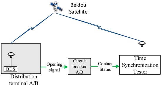
Figure 7.
Distribution network load synchronous transfer control time accuracy test.
The experiment simulated load transfer scenarios following distribution network faults. Both the original power source switch S1 and the target power source switch S2 were controlled by distribution terminals, with both terminals acquiring synchronized clocks via the GSS7000. When a main grid fault occurred, S1 had to be opened first, followed by closing S2, to ensure no circulating currents were present.
5.3.2. Experimental Protocol Design
To more comprehensively characterize the experimental conditions, this physical test was conducted under loaded conditions. The applied load matched the simulation model settings (active power of 300 kW, reactive power of 130 kvar), corresponding to a steady-state current of approximately 850 A. The experiment employed a VS1-12 vacuum circuit breaker, whose rated parameters (12 kV/1250 A/31.5 kA) fully encompassed the experimental current range. To prioritize verification of the timing coordination mechanism within the “prediction-control” closed-loop system, the most typical single-phase ground fault scenario in distribution networks was selected as the representative test case. Monitoring was performed using a high-sampling-rate oscilloscope.
The experimental procedure is as follows:
- (1)
- Before starting the test, first ensure that both power distribution terminals are synchronized and operating stably for over 10 min under the synchronized time reference output by the satellite signal simulator to establish a reliable synchronized state.
- (2)
- During testing, the master station system issues control commands with absolute timestamps to distribution terminal A (to open the original power source switch S1) and distribution terminal B (to close the target power source switch S2) based on the switching times predicted by the Bo-BiLSTM model and the calculated dynamic delay, following the “open first and then close” timing logic.
- (3)
- Critical timing points during the switching operation—specifically, the precise moment when breaker A’s contacts open and the precise moment when breaker B’s contacts close—are captured and recorded in parallel by a high-precision time synchronization tester. This tester also receives the time reference from the satellite signal simulator, ensuring that its recorded data aligns perfectly with the distribution terminal’s timeline to eliminate system timing errors. To quantitatively assess control precision, the time difference between Circuit Breaker A’s opening moment and Circuit Breaker B’s closing moment is calculated. This value represents the actual opening-closing time interval.
- (4)
- The aforementioned test procedure is repeated 100 times to obtain statistically significant results and verify the consistency and reliability of the control strategy across different operations.
5.3.3. Experimental Data Analysis
In all 100 physical experiments, the closing-to-opening time difference consistently fell within the range of 2 ms to 12 ms, with each result strictly meeting the engineering safety threshold of less than 20 ms. The experimental findings conclusively demonstrate that the proposed control strategy reliably maintained the time difference within a narrow range far below the safety upper limit, fundamentally eliminating the risk of circulating currents caused by asynchronous closing. For specific data, see Appendix A, Table A3.
5.3.4. Experimental Conclusions
This paper validated the Bo-BiLSTM-based synchronous load transfer control method for distribution networks through 100 repeated experiments. The experimental results demonstrated the following:
- High Precision and Safety: In all experimental rounds, the time difference between opening and closing operations was strictly controlled within 2–12 ms. This result not only fully meets the engineering safety requirement of less than 20 ms but also demonstrates that the system possesses sufficient performance margin, fundamentally avoiding the risk of circulating currents caused by asynchronous closing.
- Exceptional Reliability: No noticeable contact bounce was observed in all 100 repeated operations. All 100 experiments successfully achieved safe transfer, demonstrating that this control strategy exhibited high reliability and consistency rather than merely coincidental effectiveness.
- Effectiveness of the Predictive-Control Closed Loop: The experiment successfully validated the effectiveness of the dynamic delay control strategy designed based on Bo-BiLSTM high-precision time prediction, achieving a closed loop from “precise sensing” to “precise control.” This provides a reliable technical solution for seamless and rapid load transfer in distribution networks following faults.
6. Conclusions
This study proposes a switch timing prediction and synchronous control method for distribution networks based on Bayesian optimization of bidirectional long short-term memory (Bo-BiLSTM) networks. The main contributions of this work are summarized as follows:
- A Novel Prediction Model for Switching Times
We propose a Bo-BiLSTM-based prediction model that automatically adapts hyperparameters of bidirectional long short-term memory networks by integrating Bayesian optimization techniques. This approach effectively addresses challenges posed by high data dispersion and scarce training samples, significantly improving prediction accuracy and generalization capabilities compared to standard BiLSTM and LSTM models as well as XGBoost models.
- 2.
- A Comprehensive and Publicly Accessible Feature Database
We constructed a robust simulation model of a distribution network with distributed generation using MATLAB/Simulink. A comprehensive database containing 620 operational scenarios was established, encompassing various short-circuit fault types, locations, and transition resistances. This database provides a solid foundation for model training and future research in the field.
- 3.
- An Innovative Integrated Framework from Prediction to Control
We innovatively bridged the gap between accurate prediction and practical control by integrating the switch timing predictions into a load transfer control strategy. A “open first and then close” synchronous transfer control strategy with a dynamic delay mechanism was designed, ensuring seamless and safe load transfer.
- 4.
- Experimental Validation with High Practicality
The effectiveness and reliability of the proposed control strategy were rigorously validated through physical experiments. Experimental results demonstrated that the time difference between opening and closing was consistently controlled within a range of 2–12 ms, fully meeting the stringent engineering requirement of less than 20 ms and effectively mitigating the risk of circulating currents.
In summary, this method provides a reliable fault response and rapid self-healing control solution for distribution networks with high penetration of distributed energy. Future research can be further deepened in the following areas: First, advancing the model’s application to real-world data is central to our next steps. We will focus on collecting high-resolution operational data from multiple actual distribution network feeders to validate and optimize the model’s predictive performance in complex real-world environments. Second, we will explore more advanced data augmentation and few-shot learning techniques to address the inherent challenge of scarce fault data in practical engineering scenarios, ensuring that the model maintains high accuracy and reliability even with limited data.
Author Contributions
Conceptualization, H.Z. and C.L.; methodology, C.L.; validation, H.Z., C.L., and W.L.; formal analysis, X.S.; investigation, Y.G.; resources, Y.G.; data curation, C.L.; writing—original draft, W.L. and C.L.; writing—review and editing, X.S.; visualization, Y.G.; supervision, H.Z.; project administration, H.Z.; funding acquisition, H.Z. All authors have read and agreed to the published version of the manuscript.
Funding
This research was funded by the project of State Grid Sichuan Electric Power Company Limited, grant number 52199723001R.
Data Availability Statement
The original contributions presented in this study are included in the article. Further inquiries can be directed to the corresponding author.
Acknowledgments
We are grateful to the reviewers for their comprehensive review of this manuscript, as well as for their insightful comments and valuable suggestions that have significantly contributed to enhancing the quality of our work.
Conflicts of Interest
Author Cheng Long was employed by the company State Grid Sichuan Electric Power Research Institute. The remaining authors declare that the research was conducted in the absence of any commercial or financial relationships that could be construed as potential conflicts of interest.
Appendix A
Table A1.
Fault characteristic data under different operating conditions.
Table A1.
Fault characteristic data under different operating conditions.
| Operating Order Number | VA/(V) | VB/(V) | VC/(V) | IA/(A) | IB/(A) | IC/(A) | T/(ms) |
|---|---|---|---|---|---|---|---|
| O1 | 28,140 | 28,760 | 28,780 | 106.4 | 40.78 | 35.07 | 26.04 |
| O2 | 28,750 | 27,500 | 28,790 | 33.38 | 276.7 | 42.67 | 37.60 |
| O3 | 28,730 | 28,740 | 28,730 | 35.99 | 36.01 | 35.99 | 31.70 |
| O4 | 28,730 | 28,750 | 26,540 | 36.92 | 36.35 | 388.9 | 16.85 |
| O5 | 28,740 | 28,790 | 27,970 | 40.8 | 37.22 | 119.2 | 27.73 |
| ⁝ | ⁝ | ⁝ | ⁝ | ⁝ | ⁝ | ⁝ | ⁝ |
| O620 | 28,730 | 27,250 | 25,710 | 35.96 | 574.3 | 542.7 | 36.889 |
Table A2.
Standardized database of feature matrices.
Table A2.
Standardized database of feature matrices.
| VA | VB | VC | IA | IB | IC | |
|---|---|---|---|---|---|---|
| O1 | 0.4144 | 0.9822 | 0.9911 | −0.8120 | −0.9799 | −0.9945 |
| O2 | 0.6390 | 0.4209 | 0.9956 | −0.9988 | −0.3763 | −0.9751 |
| O3 | 0.6317 | 0.9733 | 0.9689 | −0.9921 | −0.9921 | −0.9921 |
| O4 | 0.6317 | 0.9777 | −0.0044 | −0.9898 | −0.9912 | −0.0893 |
| O5 | 0.6354 | 0.9955 | 0.6311 | −0.9798 | −0.9890 | −0.7793 |
| ⁝ | ⁝ | ⁝ | ⁝ | ⁝ | ⁝ | ⁝ |
| O620 | 0.6317 | 0.3096 | −0.3733 | −0.9922 | 0.3850 | 0.3042 |
Table A3.
Accuracy test data for timed action of distribution terminals.
Table A3.
Accuracy test data for timed action of distribution terminals.
| No. | The Moment When Circuit Breaker A Opens | The Closing Time of Circuit Breaker B | Time Difference (ms) | Is the Difference Between the Switch Operation Time and the Model Prediction Time Less than 0.1 ms? |
|---|---|---|---|---|
| 1 | 8:50:27.244 | 8:50:27.251 | 7 | Yes |
| 2 | 8:52:51.831 | 8:52:51.841 | 10 | Yes |
| 3 | 9:04:10.433 | 9:04:10.443 | 10 | Yes |
| 4 | 9:09:11.311 | 9:09:11.316 | 5 | Yes |
| 5 | 9:15:10.211 | 9:15:10.223 | 12 | Yes |
| 6 | 9:20:20.430 | 9:20:20.433 | 3 | Yes |
| 7 | 9:25:40.556 | 9:25:40.559 | 3 | Yes |
| 8 | 9:29:30.466 | 9:29:30.477 | 11 | Yes |
| 9 | 9:35:10.876 | 9:35:10.879 | 3 | Yes |
| 10 | 9:40:20.431 | 9:40:20.438 | 7 | Yes |
| 11 | 10:50:27.244 | 10:50:27.251 | 7 | Yes |
| 12 | 10:20:20.430 | 10:20:20.438 | 8 | Yes |
| 13 | 10:25:47.556 | 10:25:47.559 | 3 | Yes |
| 14 | 10:29:30.466 | 10:29:30.477 | 11 | Yes |
| 15 | 10:15:10.211 | 10:15:10.223 | 12 | Yes |
| 16 | 10:20:20.430 | 10:20:20.439 | 9 | Yes |
| 17 | 10:25:40.556 | 10:25:40.558 | 2 | Yes |
| 18 | 10:29:30.466 | 10:29:30.477 | 11 | Yes |
| 19 | 10:35:10.876 | 10:35:10.879 | 3 | Yes |
| 20 | 10:40:20.431 | 10:40:20.438 | 7 | Yes |
| ⁝ | ⁝ | ⁝ | ⁝ | ⁝ |
| 100 | 21:24:40.556 | 21:24:40.558 | 2 | Yes |
References
- Jiang, J.; Xin, P.; Xiao, N.; Li, Q. A Multi-Domain Protection for Reliable Slicing in Network Coding Based 5G/B5G RAN Enabled Power Distribution Network. In Proceedings of the 2024 22nd International Conference on Optical Communications and Networks (ICOCN), Harbin, China, 26–29 July 2024; pp. 1–3. [Google Scholar] [CrossRef]
- Li, X.; Yao, Z.; Zhou, L.; Zhou, S. Dispersed operating time control of a mechanical switch actuated by an ultrasonic motor. J. Vibroeng 2018, 20, 321–331. [Google Scholar] [CrossRef]
- Zhang, J.; Wang, P.; Yan, R.; Gao, R.X. Long short-term memory for machine remaining life prediction. J. Manuf. Syst. 2018, 48, 78–86. [Google Scholar] [CrossRef]
- Gugulothu, N.; Tv, V.; Malhotra, P.; Vig, L.; Agarwal, P.; Shroff, G. Predicting remaining useful life using time series embed-dings based on recurrent neural networks. Int. J. Progn. Health Manag. 2018, 9. [Google Scholar] [CrossRef]
- Lu, Q.; Polyzos, K.D.; Li, B.; Giannakis, G.B. Surrogate modeling for Bayesian optimization beyond a single Gaussian process. IEEE Trans. Pattern Anal. Mach. Intell. 2023, 45, 2891–2904. [Google Scholar] [CrossRef] [PubMed]
- Burke, J.; King, S. Edge tracing using Gaussian process regression. IEEE Trans. Image Process. 2021, 31, 138–148. [Google Scholar] [CrossRef] [PubMed]
- Hochreiter, S.; Schmidhuber, J. Long short-term memory. Neural Comput. 1997, 9, 1735–1780. [Google Scholar] [CrossRef] [PubMed]
- Babu, G.S.; Zhao, P.; Li, X.-L. Deep Convolutional Neural Network Based Regression Approach for Estimation of Remaining Useful Life. In Database Systems for Advanced Applications, Proceedings of the 21st International Conference, DASFAA 2016, Dallas, TX, USA, 16–19 April 2016; Navathe, S., Wu, W., Shekhar, S., Du, X., Wang, X., Xiong, H., Eds.; Lecture Notes in Computer Science; Springer: Cham, Switzerland, 2016; Volume 9642. [Google Scholar] [CrossRef]
- Guo, L.; Lei, Y.; Li, N.; Xing, S. Deep convolution feature learning for health indicator construction of bearings. In Proceedings of the 2017 Prognostics and System Health Management Conference (PHM-Harbin), Harbin, China, 9–12 July 2017; pp. 318–323. [Google Scholar] [CrossRef]
- Zhang, S.; Wang, L.; Zhu, M.; Chen, S.; Zhang, H.; Zeng, Z. A Bi-directional LSTM Ship Trajectory Prediction Method based on Attention Mechanism. In Proceedings of the 2021 IEEE 5th Advanced Information Technology, Electronic and Automation Control Conference (IAEAC), Chongqing, China, 12–14 March 2021; pp. 1987–1993. [Google Scholar] [CrossRef]
- Guan, L.; Qiao, F.; Zhai, X.; Wang, D. Model Evolution Mechanism for Incremental Fault Diagnosis. IEEE Trans. Instrum. Meas. 2022, 71, 3522111. [Google Scholar] [CrossRef]
- Liu, X.; Yan, F.; Song, C.; Yin, X.; Wang, Y. A research on Bayesian optimisation of bilstm neural network algorithms-application to photovoltaic power prediction. In Proceedings of the 2024 4th International Conference on Neural Networks, Information and Communication Engineering (NNICE), Guangzhou, China, 19–21 January 2024; pp. 1544–1547. [Google Scholar] [CrossRef]
- Dong, E.; Guo, Y. The Bayesian CNN-LSTM Mixed Hybrid Algorithm Model of the Photovoltaic Short-term Output Forecasting. In Proceedings of the 2023 3rd International Conference on New Energy and Power Engineering (ICNEPE), Huzhou, China, 24–26 November 2023; pp. 242–246. [Google Scholar] [CrossRef]
- Ma, Y.; He, Y.; Wang, L.; Zhang, J. Probabilistic reconstruction for spatiotemporal sensor data integrated with Gaussian process regression. Probabilistic Eng. Mech. 2022, 69, 103264. [Google Scholar] [CrossRef]
- Hodson, T.O. Root mean square error (RMSE) or mean absolute error (MAE): When to use them or not. Geosci. Model Dev. Discuss. 2022, 15, 5481–5487. [Google Scholar] [CrossRef]
- Alturki, Y.A.; Alhussainy, A.A.; Alghamdi, S.M.; Rawa, M. A novel point of common coupling direct power control method for grid integration of renewable energy sources. Energies 2024, 17, 5111. [Google Scholar] [CrossRef]
- Raj, R.D.A.; Bhattacharjee, S. Short-circuit fault analysis of three-phase grid integrated photovoltaic power system. In Proceedings of the 2020 International Conference on Power Electronics & IoT Applications in Renewable Energy and its Control (PARC), Mathura, India, 28–29 February 2020; pp. 231–236. [Google Scholar] [CrossRef]
- Jiang, W.-J.; Kim, C.-W.; Goi, Y.; Zhang, F.-L. Data normalization and anomaly detection in a steel plate-girder bridge using LSTM. ASCE-ASME J. Risk Uncertain. Eng. Syst. Part A Civ. Eng. 2022, 8, 2022. [Google Scholar] [CrossRef]
- Ran, J.; Cui, Y.; Xiang, K.; Song, Y. Improved runoff forecasting based on time-varying model averaging method and deep learning. PLoS ONE 2022, 17, e0274004. [Google Scholar] [CrossRef]
Disclaimer/Publisher’s Note: The statements, opinions and data contained in all publications are solely those of the individual author(s) and contributor(s) and not of MDPI and/or the editor(s). MDPI and/or the editor(s) disclaim responsibility for any injury to people or property resulting from any ideas, methods, instructions or products referred to in the content. |
© 2025 by the authors. Licensee MDPI, Basel, Switzerland. This article is an open access article distributed under the terms and conditions of the Creative Commons Attribution (CC BY) license (https://creativecommons.org/licenses/by/4.0/).