Abstract
Accurately predicting the fatigue life of long-distance natural gas pipelines with internal corrosion defects is essential to ensure structural integrity and operational safety. While data-driven models offer potential in this regard, many lack interpretability. To address this, we propose a novel, interpretable machine learning framework that combines an Extreme Gradient Boosting (XGBoost, v3.0.3) model, optimized via Particle Swarm Optimization (PSO), with SHapley Additive exPlanations (SHAP) based post hoc interpretation. A dataset of 510 samples was generated through FE simulations, incorporating realistic pipe geometry, material properties, and statistically representative corrosion defect parameters. The optimized PSO-XGBoost model demonstrated exceptional predictive performance on the test set, with a coefficient of determination (R2) of 0.9921, and a Mean Absolute Error (MAE) of 2.7491 years, significantly outperforming benchmark models. Crucially, the SHAP analysis provided global and local interpretations, revealing that the defect width coefficient (k3) and pipe diameter (D) are the most influential features, while operational pressure (P) had a minimized impact due to multicollinearity handling. The research findings can provide a basis for pipeline risk assessment and integrity management.
1. Introduction
Against the backdrop of the global energy transition, natural gas has garnered significant attention due to its cleanliness and has become a crucial option for achieving net-zero emissions [1,2]. Compared with traditional energy sources such as coal, natural gas combustion produces less carbon dioxide, helping to mitigate climate change [3]. It is projected that by 2025, China’s natural gas production will exceed 230 billion m3 [4]. As a key infrastructure for natural gas transportation, long-distance pipelines are continuously expanding in scale. However, these pipelines are usually buried deep underground, making them highly concealed and difficult to detect in case of failure. Accurate prediction of pipeline failures is essential for ensuring safe operation [5].
With the increasing service life of long-distance natural gas pipelines, corrosion has become a major threat to their integrity [6,7]. Corrosion defects can significantly weaken the pipe strength, leading to leaks or ruptures [8]. Existing research has primarily focused on external corrosion. For instance, Cai [9,10,11] analyzed the ultimate strength of defective pipelines through full-scale experiments and finite element simulations; Choi [12] proposed a method for evaluating the ultimate load of corroded areas in X65 steel pipes based on burst tests; and Netto [13] used numerical models to study the impact of external corrosion on burst pressure. With advancements in external anti-corrosion technologies, external corrosion has been relatively well-controlled [14]. However, internal corrosion has become increasingly prominent due to the absence of internal coatings in pipelines and the influence of transported media, yet related research remains insufficient.
Natural gas pipeline networks are characterized by multiple gas sources and diverse end-users, resulting in complex system topologies. Time-varying operating conditions, fluctuations in gas supply, and changes in user demand subject pipelines to cyclic loading, leading to cumulative fatigue damage that affects structural integrity [15]. While established assessment standards such as ASME B31G, RSTRENG, and DNV-RP-F101 [16,17,18] provide guidance for evaluating corroded pipelines under static loads, they offer limited coverage for fatigue-related degradation under alternating stresses. Dakhel [19] assessed the lifespan of welded pipelines through high-cycle fatigue experiments, though such physical testing is often costly and time-consuming [20]. Finite element-based fatigue simulation has emerged as an efficient alternative [21]. For instance, Bagni [22] applied nCode to evaluate the lifetime of welded joints, and Miao [23] simulated the influence of corrosion pits on fatigue performance. Nevertheless, there remains a lack of systematic studies addressing stress concentration and failure thresholds in internally corroded pipe segments under cyclic loading conditions [24].
Traditional failure prediction methods rely on burst tests and numerical simulations [25]. The former carries high risks and costs, while the latter is limited by defect diversity and parameter coupling, resulting in limited prediction accuracy [26]. In recent years, machine learning methods have effectively identified key failure factors through data-driven approaches, significantly improving prediction capabilities. Algorithms such as linear regression, neural networks, and XGBoost have shown potential in pipeline engineering [27]. XGBoost addresses overfitting and efficiency issues through regularization and parallel computing [28], making it particularly suitable for failure prediction under complex defect conditions [29,30]. Machine learning provides a promising complement to traditional fatigue life estimation methods, enabling faster iteration and generalization, offering rapid estimates to guide decision-making, while also complementing traditional simulations. Ángel Ladrón [31] proposed a machine learning-based process to estimate fatigue life at different wing locations based on flight parameters for various tasks, applying this approach throughout the entire service life. Konstantinos Arvanitis [32] and others explored four techniques: polynomial regression, support vector regression (SVR), XGB regression, and artificial neural networks (ANN) for predicting the fatigue life of structural steel, with results indicating that XGB regression performed better. However, machine learning models are often regarded as “black boxes”, lacking interpretability, which affects the credibility of prediction results [33].
To enhance interpretability, interpretable machine learning methods have emerged [34], including both local and global interpretation techniques [35]. LIME (Local Interpretable Model-agnostic Explanations) and SHAP are two commonly used tools [36]. SHAP [37], proposed by Lundberg et al., is a game theory-inspired method that combines both local and global analysis capabilities. Although LIME is highly adaptable, it only supports local interpretation, may overlook feature correlations during feature sampling, and requires substantial computational resources [38]. Michael A. Kraus [39] combined automated machine learning (Auto ML) with SHAP to establish an analytical process for predicting the fatigue strength of welded transverse stiffener details, demonstrating that such a process can reduce the number of simulations, lower the required computational and human resources, and provide accurate predictions.
Based on the above analysis, this paper proposes a modeling approach that integrates finite element simulation and machine learning. First, a dataset of pipeline fatigue failures under various operating conditions and defect sizes is constructed through finite element calculations. Then, ML algorithms are employed to predict the lifespan, and methods such as SHAP are used to visualize the prediction process, thereby enhancing the credibility of the results. This study is the first to apply an interpretable machine learning framework to the specific and under-researched engineering problem of fatigue life prediction for internal corrosion defects in long-distance natural gas pipelines. It combines finite element simulation, intelligent optimization, and SHAP to provide a highly accurate prediction process. The research findings can provide a basis for pipeline risk assessment and integrity management. The machine learning model constructed in this study is entirely based on finite element simulation data. Although simulation data can systematically cover a wide range of defect parameter combinations, its predictive performance still needs to be further validated and calibrated in the future using actual pipeline inspection data.
2. Materials and Methods
2.1. Material Properties
The target pipelines investigated in this study comprise X70 and X80 steel grades. Table 1 presents the true stress–strain curves and mechanical properties of X70 and X80 pipeline steel at room temperature.

Table 1.
Mechanical properties of pipeline steels.
Literature [40] indicates that “Structural Steel BS4360 Grade 40B” in nCode can be used for simulation. The S-N curve of this material is shown in Figure 1a, fitted using the software’s built-in fitting method. This study adopts the fatigue characteristic calculation method provided by the Chinese standard [41]. For X80 steel with a tensile strength of 739 MPa, the reference data points for “unalloyed and low-alloy steels not exceeding 370 °C” were selected for interpolation calculations. After interpolation processing, standardized fatigue characteristic parameters were obtained. Using data fitting methods, the S-N curve for X80 was established, as shown in Figure 1b.
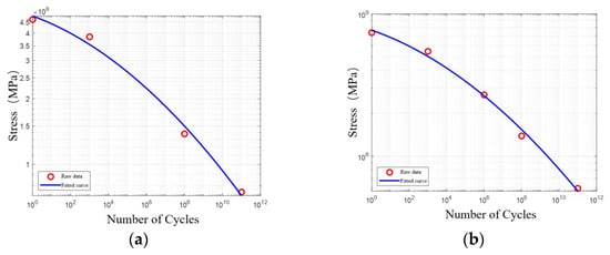
Figure 1.
S-N curve: (a) X70; (b) X80.
It can be intuitively observed from Figure 1 that the main difference between the two curves is that the S-N curve of X80 steel is entirely located above that of X70. This indicates that X80 steel exhibits superior fatigue performance across the entire high-cycle fatigue life range. In the high-life region, the gap between the two curves is relatively small; as the stress amplitude increases and the life decreases, the distance between them gradually widens. This implies that under the long-term alternating loads commonly encountered in pipeline operations, the fatigue performance advantage of X80 steel diminishes.
2.2. FE Modeling
The finite element simulation of fatigue life comprises five fundamental steps: First, engineering data is collected and field measurements are conducted on specific long-distance pipelines to obtain information such as pipe diameter, wall thickness, corrosion defect dimensions, and operational pressure fluctuations. Next, based on pipeline and defect parameters, the value ranges for FE simulation are determined, and a load spectrum is established by analyzing pipeline pressure fluctuations. Subsequently, static analysis based on the FE Method is performed to derive the stress distribution under constant pressure, thereby obtaining the stress spectrum. Then, within the fatigue failure calculation engine, utilizing cumulative fatigue damage theory, the S-N curve, and the stress spectrum, the fatigue life of pipelines with different specifications, materials, and defect characteristics is determined. Finally, fatigue vibration experiments are used to validate and optimize the prediction results. The overall process of finite element simulation is shown in Figure 2.
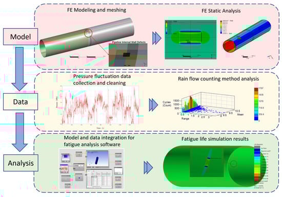
Figure 2.
FE analysis steps. In the software interface of the analysis module, (a) input the time series that have been drift-removed and deburred. In (b), adjust the material properties and fatigue calculation method. After completing the configuration, perform the calculation, and through the post-processing module, extract (c) the fatigue damage distribution cloud map and (d) the life prediction results.
This study employs the SpaceClaim module within Ansys Workbench for modeling. The specific pipeline parameters are listed in Table 2. To balance computational cost with result accuracy, the model length was set to six times the pipe diameter, a distance sufficient per Saint-Venant’s principle to isolate the defect-area stress field from boundary effects. Both ends were assigned frictionless supports (constrained radially and circumferentially, free axially) to approximate an infinitely long pipeline. This boundary condition permits axial deformation under pressure, mimicking real pipeline behavior and preventing spurious stresses from fully fixed constraints. Given the axisymmetric nature of the pipeline, a hexahedral mesh with good numerical stability and convergence is adopted. A mesh sensitivity analysis was performed to guarantee that the simulation outcomes were independent of the mesh density. The element size in the defect area was varied from 5 mm down to 0.5 mm. Figure 3 illustrates the findings, where the maximum von Mises stress at 10 MPa internal pressure and the required computation time served as the evaluation metrics.
Table 2.
Geometric and material parameters of the pipelines.
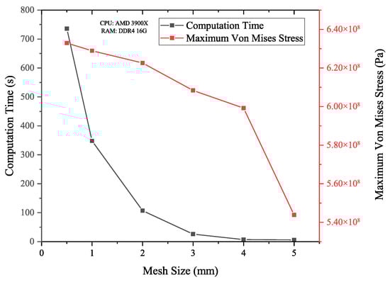
Figure 3.
Mesh independence test results.
The data reveals that stress fluctuations remain below 3% for mesh sizes between 3 mm and 0.5 mm. Balancing accuracy and computational effort, a 2 mm mesh was chosen. This configuration resulted in a model with 192,576 nodes and 93,600 elements under the tested conditions.
The dimensions of internal corrosion defects in this study were selected based on the results of two in-line inspections conducted in 2015 and 2023 on a section of the Sichuan-East Natural Gas Pipeline, a typical long-distance natural gas pipeline project in China. This pipe section utilizes steel pipe with a diameter of 1016 mm, wall thickness of 21 mm, design pressure of 10 MPa, and material X70. A total of 555 corrosion defects were identified in the two inspections. Among the 165 defects found in 2015, the length ranged from 8 to 247 mm, width from 15 to 273 mm, and depth from 1% to 10% (relative to wall thickness, same below). Among the 390 corrosion defects found in 2023, the length ranged from 10 to 70 mm, width from 10 to 305 mm, and depth from 1% to 13%. The maximum depth of defects detected in 2023 has increased, reflecting the accumulation of corrosion in the pipeline during actual operation. In generating defect parameters for finite element simulation, this study incorporates all data from two inspections to ensure that the dataset reflects the potential development range of corrosion defects over the entire lifecycle of the pipeline.
According to the inspection results, corrosion pits are mostly planar, often due to the slowing development rate of pit depth. The areas around the pit openings become activated, and under the influence of activation and passivation, the pit openings expand, with increased length and width. The morphology of the pits evolves into open-type pits, where the corrosion depth is roughly consistent within the corroded area. For ease of calculation, the pits are simplified as square defects for three-dimensional modeling. The geometric description of the model is shown in Figure 4.
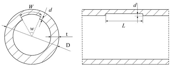
Figure 4.
Cross-section and longitudinal section of pipeline containing square corrosion defects. In this figure, D denotes the pipeline diameter, d is the defect corrosion depth, L is the axial corrosion length, W is the circumferential corrosion width.
To facilitate parallel comparison, a unified metric system was established to characterize the size of internal pipeline defects. When determining the characteristics of corrosion defects, the corrosion defect depth coefficient k1, corrosion defect length coefficient k2, and corrosion defect width coefficient k3 are employed. The definitions of these three parameters are as follows:
Based on the inspection data, the defect length follows a Gamma distribution (Equation (2)), the defect width follows an exponential distribution (Equation (3)), and the defect depth percentage follows a Beta distribution (Equation (4)).
Based on the aforementioned distribution laws, 50 sets of defect length, width, and depth parameters conforming to the statistical characteristics were randomly generated; simultaneously, 25 sets of parameters outside the high-frequency region of the distributions were selected as supplements; additionally, according to the value ranges of defect length, width, and depth, 27 sets of structured parameter combinations for finite element simulation were designed based on the principle of equal spacing.
This study selected operational pressure data from one year for the aforementioned pipe section, with a sampling frequency of 1 Hz. The data, recorded at 1 Hz for 365 days, was averaged per second. Using a two-day interval as the time history unit and after removing abnormal data, a load spectrum consisting of 159,091 data points was obtained. Based on this load spectrum, the stress ratio is R = 0.7. When applied to the pipelines intended for simulation in this study, for pipelines with a design pressure of 12 MPa, the maximum fluctuating internal pressure is 10.9 MPa and the minimum is 7.66 MPa; for pipelines with a design pressure of 10 MPa, the maximum fluctuating internal pressure is 9.1 MPa and the minimum is 6.4 MPa. The determination of a single stress ratio (R = 0.7) stems from the analysis of the actual pressure fluctuations over a one-year period in the target pipeline segment. The vast majority of pressure cycles have stress ratios concentrated around 0.7. Therefore, selecting this representative value helps us, in the initial stage of the research, focus on the influence of geometric defect morphology and material properties—the two core variables—on fatigue life, thereby controlling computational complexity. Given the sensitivity of second-level operational pressure data, the range of parameters considered in this study is limited. Investigating the effects of different stress ratios is highly valuable, and we have identified it as a key direction for future research.
2.3. Collected Data
Through finite element modeling, this study developed a dataset containing 510 “geometric parameter-fatigue life” samples. To balance model accuracy and computational cost, this study adopted a compromise approach in the data generation strategy, generating simulated data based on the actual probability distribution of defect sizes and introducing moderate deviations to enhance diversity. The resulting 510 samples cover a wide distribution of pipeline specifications and defect parameters, which is sufficient for training a robust regression model. Table 3 shows the summary information for each variable. The defect size parameters k1, k2, and k3 used in this study are normalized coefficients, and their corresponding actual physical size ranges are as follows: the distribution range of defect depth d is from 0.364 mm to 23.76 mm, with a mean of 2.51 mm; the distribution range of defect length L is from 13.60 mm to 358.78 mm, with a mean of 67.88 mm; the distribution range of defect width W is from 11.17 mm to 559.76 mm, with a mean of 140.68 mm.
Table 3.
Summary basic information of database.
Figure 5 displays the distribution of input and output variables and their pairwise relationships, revealing correlations and potential relationships between variables. Features (Lines 1~9) are pipe diameter D (mm), wall thickness δ (mm), operational pressure P (MPa), yield strength σy (MPa), ultimate tensile strength σu (MPa), defect depth coefficient k1, defect length coefficient k2, defect width coefficient k3, and defect aspect ratio k2/k3, respectively. Feature line 10 is the fatigue life Tyear (years).
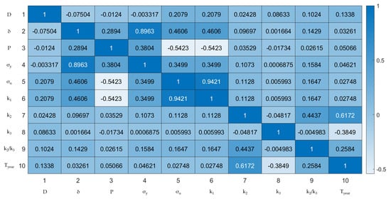
Figure 5.
Result of correlation coefficients between input variables.
3. Model Description
3.1. Implementation Methodology
To achieve high-precision prediction and visualization of the prediction process for the fatigue life of long-distance natural gas pipelines with internal corrosion defects, this paper proposes a novel method based on PSO-XGBoost-SHAP. Figure 6 illustrates the analytical framework of this model, with the specific steps as follows.
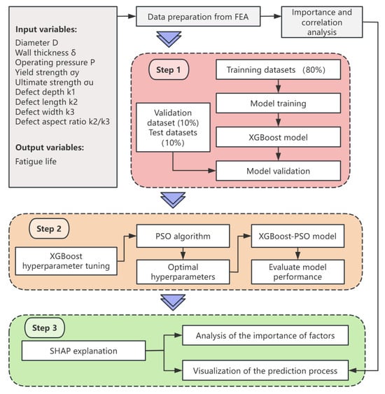
Figure 6.
The flowchart of PSO-XGBoost-SHAP.
- Step 1: Model Construction and Comparison. After data collection and preprocessing, the dataset is randomly divided into a training set (80% of samples), a validation set (10% of samples), and a test set (10% of samples). The XGBoost model is applied to learn from the training set, establishing a fatigue life prediction model for long-distance pipelines with defects. To evaluate the applicability of the XGBoost model, its prediction results and performance metrics are compared with those of other common models on the test set;
- Step 2: Model Optimization. The performance of machine learning models is influenced by various factors such as data quality and hyperparameter settings. This step focuses on optimizing the XGBoost model via the PSO algorithm, fine-tuning its hyperparameters to enhance predictive performance. The impact of key PSO parameters on model performance is analyzed, and the sensitivity of XGBoost hyperparameters to predictive performance is evaluated to determine the optimal configuration;
- Step 3: Enhancing Interpretability with SHAP. The SHAP method is employed to quantify the contribution of each feature to the model’s prediction. By calculating the SHAP value for each feature, the influence of each variable on the final prediction is assessed, determining whether it pushes or inhibits the model output. The SHAP analysis is compared with the previously mentioned Pearson correlation coefficient results to confirm the reliability of the model’s predictions.
3.2. XGBoost
XGBoost is an enhanced algorithm of Gradient Boosting Decision Trees (GBDT) that introduces a series of innovative techniques in training speed and model performance. The flowchart of XGBoost is shown in Figure 7. Let the training dataset D = {(x1, y1), (x2, y2), …, (xN, yN)}, where xi is the input feature and yi is the corresponding label.
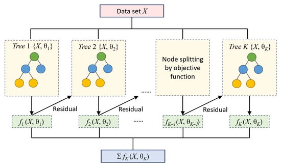
Figure 7.
Schematic diagram of the XGBoost algorithm. In this figure, different colored circles represent hierarchical nodes of a decision tree.
The objective of XGBoost is to train the model by minimizing the loss function. The loss function consists of two parts: the loss term and the regularization term:
where represents the cumulative result of the model from the previous t-1 rounds, and represents the prediction of the weak learner in the t-th iteration. The regularization term includes the L2 regularization of the leaf node weights and the L1 regularization of the number of leaf nodes.
To fit the loss function more accurately, XGBoost employs a second-order Taylor expansion. The negative gradient is defined as the residual:
In XGBoost, the calculation of the residual considers the number of samples in the leaf node where the sample resides:
where is the number of samples in the leaf node j where sample i resides at the (t-1)-th iteration, and λ is a smoothing term. In the t-th iteration, a weak learner is trained by fitting the residual. The training objective is:
where is the regularization term used to control the complexity of the decision tree.
The new learner is integrated into the model via the learning rate:
This process iterates until a predetermined number of iterations is reached or the loss function converges. The final model is represented as the cumulative sum of all weak learners:
Thus, XGBoost introduces richer regularization terms compared to GBDT, including L2 regularization of leaf node weights and L1 regularization of the number of leaf nodes. This makes XGBoost more flexible in preventing overfitting. Additionally, XGBoost uses second-order Taylor expansion to fit the loss function more accurately and employs optimization techniques to improve training efficiency. This makes XGBoost potentially more suitable for complex loss functions and high-dimensional sparse data.
Quantitative evaluation of model prediction performance is an essential part of the modeling analysis process, used to assess the model’s predictive capability and judge the applicability and reasonableness of the predictive model. To facilitate comparison of the predictive performance of machine learning models, two performance metrics are used in linear and nonlinear regression analysis: Mean Absolute Error (MAE), and the Coefficient of Determination (R2). The performance metrics can be expressed as:
where n is the number of samples used for testing and training; Yi, Ŷi, and Ȳ represent the actual value, predicted value, and mean of the actual values of the data, respectively. Smaller values of MAE indicate higher accuracy of the predictive model in estimating pipeline fatigue life. Conversely, an R2 value closer to 1 indicates more significant regression performance and higher accuracy of the predictive model.
3.3. PSO
After obtaining hyperparameters via maximum likelihood estimation on the training set, Particle Swarm Optimization (PSO) theory is used to optimize the hyperparameters and find the optimal set.
PSO is an abbreviation for Particle Swarm Optimization, which finds the optimal result through iteration among random particles. In a particle swarm consisting of m particles, each particle can be represented by an n-dimensional vector:
The velocity of the particle can also be represented by an n-dimensional vector:
After establishing the position and velocity of the particle swarm, the optimal position of the particle is found through iteration, represented by an n-dimensional vector:
By iteratively optimizing each particle, the optimal position of the entire particle swarm is found, represented by the vector:
The position and velocity of particle i are updated by finding the two optimal positions using the following method:
where ω is the inertia weight, t is the iteration number, c1 and c2 are learning factors, and r1 and r2 are random numbers in the interval (0, 1).
3.4. K-Fold Crossover Method
K-fold cross-validation is a widely adopted cross-validation strategy in machine learning, aimed at effectively evaluating model generalization ability and selecting the optimal model. The core process of this method involves two key steps: First, the original dataset is randomly partitioned into k subsets of approximately equal size, referred to as folds. Subsequently, in each round of validation, one of the folds is sequentially used as the test set, while the remaining k-1 folds are combined to form the training set, thereby training the model and evaluating its performance on the test set. Finally, the results from the k training and testing rounds are aggregated, typically using the average of the performance metrics as the evaluation criterion for the model’s overall capability.
In this process, the value of k has a significant impact on the evaluation outcome. If k is set too small, it may lead to insufficient training data, increasing the model estimation bias, while also resulting in higher variance in the evaluation due to stronger randomness in data partitioning. Conversely, if k is set too large, although it can reduce bias, it significantly increases computational load and time cost, and may even lead to overly optimistic evaluation due to high overlap between folds, failing to effectively reflect the model’s true generalization ability. Therefore, setting a reasonable k value is key to balancing the stability of model evaluation and computational efficiency. Considering common practices in the existing literature and the size and characteristics of the dataset used in this study, to balance evaluation robustness and computational feasibility, this study sets k to 10.
3.5. Model Interpretation Method
SHAP (SHapley Additive exPlanation) is an interpretability method based on the principle of Shapley values from cooperative game theory, aiming to quantify the contribution of each input feature to a specific prediction outcome in complex machine learning models, thereby addressing the problem of difficult-to-interpret predictions from traditional ML models. This method models a single prediction process as a cooperative game, where each input feature acts as a “player,” the difference between the model’s predicted output for the current instance and a preset baseline value is regarded as the “total gain,” and this total gain is fairly distributed to each feature according to the axiomatic framework of Shapley values, thus obtaining the contribution value of each feature to the current prediction. SHAP not only enhances model transparency and interpretability but also supports both local explanations at the individual prediction level and global explanations at the overall model behavior level: it displays the overall influence of features globally and reveals the effect of a single feature on a specific prediction locally. By quantifying feature importance, the SHAP method can highlight key variables affecting predictions, aid in feature selection, and deepen the understanding of the model mechanism, especially systematically revealing the underlying decision logic in models such as XGBoost regression. The formula for calculating Shapley values in this method is as follows:
where is the Shapley value of the i-th feature; N is the total number of features; represents the model output for the input instance S, where S is a subset of features; the above formula iterates over all possible subsets S, calculates the difference in model output when the i-th feature is added versus when it is not, and multiplies it by the corresponding weight.
The SHAP method parses the model prediction process through the calculation of SHAP values and the setting of a baseline value. Here, the baseline value represents the average level of the overall prediction, while the SHAP value quantifies the contribution of each feature to the prediction result. In the model prediction process, the baseline value is considered the starting point of the prediction result. The SHAP value then adjusts the baseline value to reflect the feature’s influence on the prediction result when considering the role of each feature. SHAP values can be positive or negative; a positive value indicates a positive influence of the feature on the prediction result relative to the baseline, while a negative value indicates a negative influence. The final predicted value is obtained by adding the SHAP value of each feature to the baseline value. This method can clearly show the relative importance of each feature to the prediction result and the prediction realization process, making the model prediction mechanism more transparent and interpretable.
4. Results and Discussion
4.1. Comparison with ML-Based Models
To confirm the reliability and effectiveness of the developed PSO-XGBoost model results, this study established multiple benchmark machine learning models for comparative analysis, including Multiple Linear Regression, Random Forest (RF), Support Vector Machine (SVM), LASSO, and XGBoost. All models were trained using 10-fold cross-validation. Figure 8 shows the comparison results of prediction accuracy (R2) and Mean Absolute Error (MAE) for these models. The PSO-XGBoost model with default parameters already possesses the highest prediction accuracy (R2 = 0.9881) and the smallest error (MAE = 3.0049). Compared to the RF, SVM, and XGBoost models, the prediction accuracy (R2) of PSO-XGBoost improved by approximately 5.1%, 4.7%, and 1.3%, respectively. The RF model performed well on the dataset, but PSO-XGBoost was superior; the XGBoost model showed high accuracy, but its performance was further improved after PSO, with the R2 value increasing from 0.97549 to 0.9881. This indicates that the PSO-optimized XGBoost model possesses excellent performance in the prediction task. From the perspective of error metrics, the MAE of the PSO-XGBoost model is 3.0049, significantly lower than other benchmark models, further verifying its superior predictive capability. To substantiate the significance of this improvement, pre-experiments were conducted to compare several optimization algorithms, including Bayesian Optimization, RIMA, and SSA, alongside PSO. Among these, PSO achieved the highest performance gain, whereas Bayesian Optimization resulted in a reduction of −1.96%, and RIMA and SSA yielded improvements of 1.18% and 0.83%, respectively. These comparative results highlight that the performance gain achieved by PSO is not only consistent but also the most pronounced among commonly used optimizers.
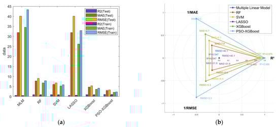
Figure 8.
Comparison of prediction accuracy and error among ML models: (a) Comparison of Machine Learning Model Performance; (b) Radar Chart Comparison of Model Performance on the Test Set (Normalized Values, Larger is Better).
Figure 9 further illustrates the correlation between predicted values and actual values for the six machine learning models under default parameters. The horizontal axis represents the actual observed values, the vertical axis represents the model predicted values, and the dark gray solid line represents the ideal prediction scenario (predicted value equals actual value). Data points closer to this trend line indicate better model prediction performance. It can be clearly observed that the prediction points of the Multiple Linear model and LASSO regression are more scattered, significantly deviating from the trend line, reflecting their poor prediction performance. In contrast, the prediction points of the PSO-XGBoost model cluster more tightly around the trend line, with deviations occurring only in a few intervals where the true value is approximately 58 and greater than 160, demonstrating overall better fitting performance and prediction robustness. In the interval of Tyear ≈ 58 (53–63 years), the main characteristics are pipeline specifications D = 1016 mm, δ = 21 mm, P = 10 MPa, and the material is X70 steel. The depth coefficient k1 ranges from 0.1 to 0.3 (moderate to relatively deep), the length coefficient k2 ranges from 0.5 to 1.5 (small to moderate length), and the width coefficient k3 ranges from 0.01 to 0.1 (moderate width). The prediction deviations in this interval may stem from two aspects: first, defects at moderate depths are in a critical state of fatigue life under specific loads, leading to increased prediction sensitivity; second, the specific combination of length, width, and depth ratios in this range may cause nonlinear special changes in the stress concentration factor. In the interval of Tyear > 160, the main characteristics are pipeline specifications D = 1016 mm, δ = 18.2 mm, and the material is X80 steel. The defect sizes are generally very small: k1 ranges from 0.02 to 0.1, k2 from 0.1 to 0.5, and k3 from 0.01 to 0.05. Therefore, the longer lifespan in this interval is due to the defect sizes being far below the critical value, while the prediction deviations may arise from inaccuracies in the finite element model’s calculations for such minor defects. Although these deviations objectively exist, the predicted fatigue life has already exceeded the design service life of most pipelines, so they have little impact on engineering applications.
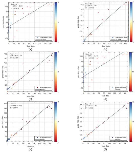
Figure 9.
Prediction results of fatigue life in training and test set: (a) Multiple Linear Model; (b) RF; (c) SVM; (d) LASSO; (e) XGBoost; (f) PSO-XGBoost.
4.2. Hyperparameter Tuning and Final Prediction Result
The hyperparameter optimization process for the PSO-XGBoost model in this study was implemented via the PSO algorithm. In practice, the K-fold cross-validation method was used to partition the original training dataset into 10 mutually exclusive subsets. Sequentially, 9 folds were used as the secondary training set and the remaining 1 fold as the secondary test set, thus constructing an evaluation framework for hyperparameter search. The main parameter settings for the PSO algorithm were as follows: Population size was 20, number of Iterations was 12, inertia weight range was [0.4, 0.9], cognitive weight was 2.0, and social weight was 2.0. Through multiple attempts, we found that 15 particles and 11 iterations were sufficient to achieve stable convergence. Further increasing the number of iterations or particles resulted in negligible improvements in outcomes but significantly increased computational time, as shown in Figure 10. To strike a balance between optimization effectiveness and computational cost, we ultimately set the number of particles to 20 and iterations to 12.
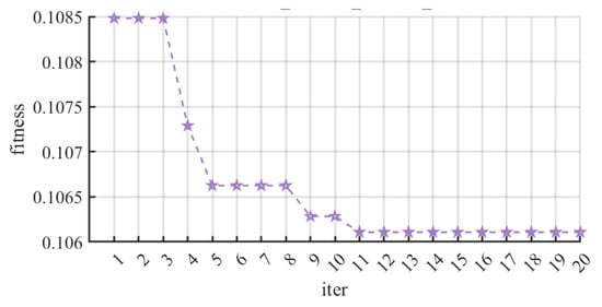
Figure 10.
PSO-XGBoost iterative process. The purple stars represent the metric of model performance at each iteration.
During the optimization process, with MAE as the optimization objective and based on the principle of minimizing cross-validation error, the optimal hyperparameter combination was searched for in the secondary training set and validated for performance in the secondary test set. The final determined hyperparameter values are shown in Table 4.
Table 4.
Hyperparameter selection.
After hyperparameter optimization, the prediction performance of the improved XGBoost model was enhanced, as shown in Figure 11. Compared to the PSO-XGBoost algorithm with default parameters in Figure 7, the goodness-of-fit of the optimized model on the test set noticeably improved. Specifically, the coefficient of determination R2 for the test set increased from the original 0.9881 to 0.9921. Particularly in the 160–200 interval, the predicted values became closer to the true observed values, indicating enhanced fitting capability for the high-value region. This improvement demonstrates the role of hyperparameter optimization in improving the prediction accuracy of machine learning models. The final R2 value on the test set is near 1, indicating that the optimized PSO-XGBoost model achieves good generalization performance and shows practical value in pipeline fatigue life prediction.
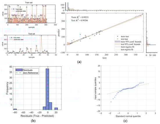
Figure 11.
Model results presentation: (a) Comparison of prediction accuracy; (b) Residual histogram; (c) Residual Q-Q plot. Blue plus symbols represent the observed residual values from the dataset. Each “+” corresponds to a single residual. Beige dash-dot line represents the theoretical quantiles of a standard normal distribution.
Figure 11b shows the residual histogram, and Figure 11c displays the residual Q-Q plot. The results indicate that the errors follow a normal distribution with no systematic bias. For the evaluation metric MAE, the model achieved an MAE of 2.7491 years. Relative to the average lifespan of 42.7 years, the relative error is approximately 6.4%. In pipeline integrity management practices, the planning of maintenance and inspection cycles is typically measured in years, often spanning 3–5 years or longer. Therefore, the prediction accuracy of this model is sufficient to provide references for risk assessment and maintenance decisions on an engineering time scale.
4.3. Model Visualization and Interpretation
In this paper, the aforementioned PSO-XGBoost model was used to predict the fatigue failure of long-distance natural gas pipelines with internal corrosion defects under fluctuating operational pressure conditions. The model’s prediction achieved an R2 of 0.9921, MAE of 2.7491, indicating that the model possesses high accuracy, goodness-of-fit, and generalization performance. However, this model is a black-box model, and its performance metrics can only partially reflect its predictive capability. To ensure the model’s reliability, it is necessary to clarify the model’s prediction mechanism and ensure its prediction process conforms to physical principles. This study employs the SHAP method to interpret this model.
The model inputs consist of 9 feature variables: D, δ, P, σy, σu, k1, k2, k3, and k2/k3, with the output being Tyear. Applying the SHAP method to interpret the prediction mechanism of this model yields the results shown in Figure 12.
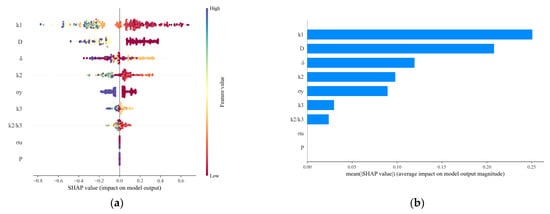
Figure 12.
Interpretation of the model’s prediction mechanism using the SHAP method: (a) SHAP Value Distribution Summary; (b) Mean SHAP Importance.
Figure 12a shows the distribution of SHAP values for different feature variables across their values for all samples. This chart clearly presents the influence patterns of different feature variables on the model prediction process globally. The feature varia-bles k1 and D have the widest distribution ranges of SHAP values, located at the top of the chart, showing substantial positive and negative impacts, indicating that they have very different effects on the model’s prediction results for different observed values.
Observing the SHAP value distribution for feature variable k1 reveals that as the k1 value increases, the SHAP value transitions from positive contribution to negative contribution, meaning larger values lead to smaller predicted values for Tyear. This indicates a negative feedback relationship between this feature variable and Tyear. It is generally believed that “the deeper the defect, the shorter the lifespan” refers to the absolute depth. However, in this study, k1 is a relative value. For a larger k1 value, it may correspond to two physical scenarios: one is “large defect, thick pipe wall,” and the other is “small defect, thin pipe wall.” The pipeline specification parameters set in this study often mean that an increase in k1 implies a greater wall thickness of the pipeline under consideration. The structural enhancement brought about by this outweighs the negative effect of the increased defect depth, resulting in a longer fatigue life, which is reflected as a negative SHAP value. The transition of the SHAP value for k1 from positive to negative corresponds to a k1 value of 0.5, meaning that when the k1 value exceeds the threshold of 0.5, the defect depth itself becomes the dominant failure factor. Regardless of the wall thickness, its severe stress concentration effect leads to a significant reduction in fatigue life, and the SHAP value consequently turns positive (shortening the lifespan). For feature variable D, as the D value increases, its SHAP value decreases, albeit with a smaller magnitude of decrease compared to k3. This suggests that an increase in the D value leads to a decrease in the predicted Tyear, and its influence is weaker than that of k1.
From a physical mechanism perspective, the reason why the defect depth coefficient k1 and the pipeline diameter D dominate the model is that they collectively determine the critical mechanical response of the pipeline under alternating loads. As a local indicator of defect severity, k1 directly controls the stress concentration level at the bottom of the corrosion pit. An increase in its value significantly accelerates the initiation and propagation of fatigue cracks, thereby exerting a nonlinear and decisive negative impact on fatigue life. Meanwhile, the pipeline diameter D, as a global geometric parameter, systematically governs the overall stress level of the pipe body through the hoop stress formula of thin-walled cylinders. A larger diameter results in higher stress under the same internal pressure, thereby accelerating the accumulation of fatigue damage. Thus, k1 and D dominate the prediction of fatigue life from the two fundamental dimensions of local defect effects and global structural response, respectively. The results of the SHAP analysis are highly consistent with this physical principle, not only validating the reliability of the model but also clearly revealing its inherent decision-making logic.
The features in the middle—δ, k2, σy, k3, and k2/k3—also display points of both colors, but the distribution of points is more concentrated, indicating a relatively smaller influence: (1) The feature variable δ exhibits a positive feedback relationship with its SHAP value. That is, as the value of δ increases, its SHAP value shows an upward trend, and the predicted value of Tyear also increases. This aligns with engineering intuition: a greater wall thickness provides a larger material load-bearing volume, reducing the nominal stress levels induced by internal pressure and defects, thereby significantly slowing the accumulation of fatigue damage and extending fatigue life. (2) For the feature variables k2 and k2/k3, both show a positive feedback relationship with their SHAP values. However, most of their SHAP values are negative, with only a few positive, suggesting that an increase in their values can only mitigate the reduction in the predicted Tyear. An increase in k2 or k2/k3 implies the growth of defects in the axial or circumferential direction, which typically exacerbates stress concentration and shortens the fatigue life. (3) For the feature variables δ, k1, and σy, the magnitude of their SHAP values exhibits a negative feedback relationship with the feature variable values, indicating that an increase in these values leads to a decrease in the predicted Tyear. The negative feedback relationship revealed by the model is consistent with the material analysis in Section 2.1, suggesting that, within the high-cycle fatigue range involved in this study, stress concentration at the defect dominates the failure process, rather than the overall strength of the material.
The features at the bottom, P and σu, have the smallest distribution ranges of SHAP values, and most of their impacts are close to zero, indicating that these feature variables contribute less to the model’s prediction and have a smaller effect on the predicted value. For the feature variable P, the low contribution of operating pressure (P) is mainly due to its multicollinearity with pipeline design parameters. During the pipeline design phase, pressure is an important indicator for determining pipe wall thickness (δ) and pipe material (reflected as σy and σu). Therefore, the operating pressure P is highly correlated with features such as δ and σy. The XGBoost algorithm inherently handles feature multicollinearity through its regularization terms (L1/L2) and tree-based splitting rules. It tends to select the most predictive representative from a set of highly correlated features while diminishing the contributions of other correlated features. In this model, the information related to P is largely captured by features such as δ and σy, resulting in a reduced SHAP importance for P itself.
Based on the absolute value of the SHAP values of feature variables in each sample prediction, the mean across all samples is calculated as the SHAP importance of that feature, as shown in Figure 12b. According to the results, the feature variables k1 and D contribute the most to the prediction results, with mean absolute SHAP values of 0.2756 and 0.2294, respectively. Due to the algorithm’s handling of multicollinearity among features, the feature variable P contributes the least to the prediction result, with a mean absolute SHAP value of 0.0182. The ranking of all feature variables by SHAP importance is: k1 > D > δ > k2 > σy > k3 > k2/k3 > σu > P. Such conclusions from the global interpretation, as well as the SHAP feature importance ranking, are consistent with the discussion in Section 2.3 on the results of correlation coefficients between input variables, demonstrating the reliability of the established combined intelligent prediction model.
5. Conclusions
This study addressed the problem of fatigue life prediction for long-distance natural gas pipelines with internal corrosion defects by proposing an interpretable machine learning modeling framework integrating PSO, XGBoost modeling, and SHAP interpretation. Through systematic finite element modeling and data generation, a database containing 510 samples of pipeline defects and fatigue life was constructed, covering multi-dimensional feature variables such as pipe diameter, wall thickness, operational pressure, material properties, and defect geometry. The research findings indicate:
- The PSO-XGBoost model demonstrated superior prediction accuracy and robustness compared to traditional machine learning models. After hyperparameter optimization, the model achieved a coefficient of determination R2 of 0.9921 and a Mean Absolute Error MAE of 2.7491 on the test set, indicating strong fitting capability and generalization performance;
- The SHAP method effectively revealed the physical mechanism behind the model’s predictions and quantified feature contributions. Global feature importance analysis identified the defect width coefficient k3 and pipe diameter D as the most significant factors affecting fatigue life prediction, while operational pressure P showed the lowest contribution due to multicollinearity handling. SHAP local explanations further clarified the positive and negative relationships between various features and fatigue life, enhancing the transparency and credibility of the prediction process;
- This study presents the first application of an interpretable machine learning framework to the specific and understudied engineering problem of fatigue life prediction for internal corrosion defects in long-distance natural gas pipelines. By integrating finite element simulation, intelligent optimization, and SHAP analysis, it provides a relatively accurate predictive workflow. The approach preliminarily demonstrates a promising and interpretable analytical framework that combines predictive capability with explanatory power.
This research also acknowledges several limitations, including reliance on syn-thetic data and lack of validation under different stress ratios. Future work should focus on experimental validation with real pipeline data, verification across varying operational conditions, and extension to more diverse defect morphologies and material types.
Author Contributions
Conceptualization, Z.N.; methodology, Z.N.; software, Z.N. and X.Z.; validation, Z.N., L.C. and C.C.; formal analysis, Z.N., L.C. and X.Z.; investigation, L.C. and C.C.; resources, L.C.; data curation, L.C. and C.C.; writing—original draft, Z.N.; writing—review and editing, L.C.; visualization, X.Z. All authors have read and agreed to the published version of the manuscript.
Funding
This research received no external funding.
Data Availability Statement
The original contributions presented in this study are included in the article. Further inquiries can be directed to the corresponding author(s).
Conflicts of Interest
Author C.C. was employed by the company Pipe China Engineering Technology Innovation Co., Ltd. The remaining authors declare that the research was conducted in the absence of any commercial or financial relationships that could be construed as a potential conflict of interest.
Abbreviations
The following abbreviations are used in this manuscript:
| X70 | API 5L Grade X70 Pipe Steel |
| X80 | API 5L Grade X80 Pipe Steel |
| PSO | Particle Swarm Optimization |
| XGBoost | EXtreme Gradient Boosting |
| SHAP | SHapley Additive exPlanation |
| R2 | R-Square |
| MAE | Mean Absolute Error |
| RMSE | Root Mean Squared Error |
| FE | Finite Element |
| ML | Machine Learning |
| LIME | Local Interpretable Model-agnostic Explanations |
References
- Abdul-Salam, Y.; Abdul-Salam, F. Qatar’s LNG exports: Advancing efficiency in electricity generation and reducing carbon emissions in the global energy transition. Energy Strat. Rev. 2025, 62, 101978. [Google Scholar] [CrossRef]
- Liu, Z.; Xu, S.; Zhao, S.; Li, Y.; Zhou, M.; Li, S.; Meng, F. Clean energy supply chain optimization: Steady-state natural gas transportation. Clean. Logist. Supply Chain 2025, 15, 100214. [Google Scholar] [CrossRef]
- Kinyar, A.; Bothongo, K.; Doytch, N. Rebound in oil and natural gas emissions amid coal-phase out: Implications for the UK’s net-zero strategy. Energy 2025, 336, 138506. [Google Scholar] [CrossRef]
- Editorial Committee of the China Natural Gas Development Report (2025). China Natural Gas Development Report (2025); Petroleum Industry Press: Beijing, China, 2025; pp. 5–10. ISBN 978-7-5183-7777-0. [Google Scholar]
- Wang, Y.; Zhang, Z.; Lu, M.; Qin, J.; Qin, G. Interpretable failure prediction modeling of hydrogen-blended natural gas pipelines containing a crack-in-corrosion defect. J. Loss Prev. Process. Ind. 2025, 98, 105744. [Google Scholar] [CrossRef]
- Gao, J.; Yang, P.; Li, X.; Zhou, J.; Liu, J. Analytical prediction of failure pressure for pipeline with long corrosion defect. Ocean Eng. 2019, 191, 106497. [Google Scholar] [CrossRef]
- Mazumder, R.K.; Salman, A.M.; Li, Y.; Yu, X. Reliability Analysis of Water Distribution Systems Using Physical Probabilistic Pipe Failure Method. J. Water Resour. Plan. Manag. 2019, 145, 1034. [Google Scholar] [CrossRef]
- Jiang, F.; Dong, S. Development of an integrated deep learning-based remaining strength assessment model for pipelines with random corrosion defects subjected to internal pressures. Mar. Struct. 2024, 96, 103637. [Google Scholar] [CrossRef]
- Cai, J.; Jiang, X.; Lodewijks, G.; Pei, Z.; Wu, W. Residual ultimate strength of damaged seamless metallic pipelines with metal loss. Mar. Struct. 2018, 58, 242–253. [Google Scholar] [CrossRef]
- Cai, J.; Jiang, X.; Lodewijks, G.; Pei, Z.; Wu, W. Residual ultimate strength of damaged seamless metallic pipelines with combined dent and metal loss. Mar. Struct. 2018, 61, 188–201. [Google Scholar] [CrossRef]
- Cai, J.; Jiang, X.; Lodewijks, G.; Pei, Z.; Zhu, L. Experimental Investigation of Residual Ultimate Strength of Damaged Metallic Pipelines. J. Offshore Mech. Arct. Eng. 2019, 141, 011703. [Google Scholar] [CrossRef]
- Choi, J.; Goo, B.; Kim, J.; Kim, Y.; Kim, W. Development of limit load solutions for corroded gas pipelines. Int. J. Pres. Ves. Pip. 2003, 80, 121–128. [Google Scholar] [CrossRef]
- ASME B31G-2012; Manual for Determining the Remaining Strength of Corroded Pipelines: Supplement to B31 Code for Pressure Piping. American Society of Mechanical Engineers (ASME): New York, NY, USA, 2012.
- AGA PR-3-805; A Modified Criterion for Evaluating the Remaining Strength of Corroded Pipe. American Gas Association (AGA): Washington, DC, USA, 1999.
- DNV-RP-F101; Recommended Practice DNV-RP-F101: Corroded Pipelines. DNV (Det Norske Veritas): Høvik, Norway, 2010.
- Netto, T.; Ferraz, U.; Estefen, S. The effect of corrosion defects on the burst pressure of pipelines. J. Constr. Steel Res. 2005, 61, 1185–1204. [Google Scholar] [CrossRef]
- Shah, B.A.; Muthalif, A.G. Muthalif. A comprehensive review on corrosion management in oil and gas pipeline: Methods and technologies for corrosion prevention, inspection and monitoring. Anticorros. Methods Mater. 2025, 75, 681–701. [Google Scholar] [CrossRef]
- Miner, M.A. Cumulative Damage in Fatigue. J. Appl. Mech. 1945, 12, 159–164. [Google Scholar] [CrossRef]
- Dakhel, A.Y.; Gáspár, M.; Koncsik, Z.; Lukács, J. Fatigue and Burst Tests of Full-scale Girth Welded Pipeline Sections for Safe Operations. Weld. World 2023, 67, 1193–1208. [Google Scholar] [CrossRef]
- Pinheiro, B.d.C.; Pasqualino, I.P. Fatigue Analysis of Damaged Steel Pipelines Under Cyclic Internal Pressure. Int. J. Fatigue 2009, 31, 962–973. [Google Scholar] [CrossRef]
- Hofman, P.; van der Meer, F.; Sluys, L. A Numerical Framework for Simulating Progressive Failure in Composite Lami-nates Under High-cycle Fatigue Loading. Eng. Fract. Mech. 2024, 295, 109786. [Google Scholar] [CrossRef]
- Bagni, C.; Halfpenny, A.; Hill, M.; Tarasek, A. A Pragmatic Approach for the Fatigue Life Estimation of Hybrid Joints. Procedia Struct. Integrity 2024, 57, 859–871. [Google Scholar] [CrossRef]
- Miao, C.; Li, R.; Yu, J. Effects of Characteristic Parameters of Corrosion Pits on the Fatigue Life of the Steel Wires. J. Constr. Steel Res. 2020, 168, 105879. [Google Scholar] [CrossRef]
- Wang, G.; Ma, Y.; Wang, L.; Zhang, J. Stress Concentration Factor Induced by Multiple Adjacent Corrosion Pits. Structures 2020, 26, 938–947. [Google Scholar] [CrossRef]
- Motta, R.S.; Cabral, H.L.; Afonso, S.M.; Willmersdorf, R.B.; Bouchonneau, N.; Lyra, P.R.; de Andrade, E.Q. Comparative studies for failure pressure prediction of corroded pipelines. Eng. Fail. Anal. 2017, 81, 178–192. [Google Scholar] [CrossRef]
- Al-Sabaeei, A.M.; Alhussian, H.; Abdulkadir, S.J.; Jagadeesh, A. Prediction of oil and gas pipeline failures through machine learning approaches: A systematic review. Energy Rep. 2023, 10, 1313–1338. [Google Scholar] [CrossRef]
- Liu, W.; Chen, Z.; Hu, Y. XGBoost algorithm-based prediction of safety assessment for pipelines. Int. J. Press. Vessels Pip. 2022, 197, 104655. [Google Scholar] [CrossRef]
- Okazaki, Y.; Okazaki, S.; Asamoto, S.; Chun, P. Applicability of machine learning to a crack model in concrete bridges. Comput. Aided Civ. Infrastruct. Eng. Eng 2020, 35, 775–792. [Google Scholar] [CrossRef]
- Wang, M.; Li, Y.; Yuan, H.; Zhou, S.; Wang, Y.; Ikram, R.M.A.; Li, J. An XGBoost-SHAP approach to quantifying morphological impact on urban flooding susceptibility. Ecol. Indic. 2023, 156, 111137. [Google Scholar] [CrossRef]
- Feng, D.-C.; Wang, W.-J.; Mangalathu, S.; Hu, G.; Wu, T. Implementing ensemble learning methods to predict the shear strength of RC deep beams with/without web reinforcements. Eng. Struct. 2021, 235, 111979. [Google Scholar] [CrossRef]
- Ángel, L.; Miguel, S.; Sánchez-Domínguez, M.; Rozalén, J.; Sánchez, F.R.; de Vicente, J.; Lacasa, L.; Valero, E.; Rubio, G. A certifiable machine learning-based pipeline to predict fatigue life of aircraft structures. Eng. Fail. Anal. 2026, 184, 110334. [Google Scholar]
- Konstantinos, A.; Pantelis, N.; Pavlou, D.; Farmanbar, M. Machine learning-based fatigue lifetime prediction of structural steels. Alex. Eng. J. 2025, 125, 55–66. [Google Scholar] [CrossRef]
- Han, T.; Siddique, A.; Khayat, K.; Huang, J.; Kumar, A. An ensemble machine learning approach for prediction and optimization of modulus of elasticity of recycled aggregate concrete. Constr. Build. Mater. 2020, 244, 118271. [Google Scholar] [CrossRef]
- Zhang, L.; Wang, L.; Ji, D.; Xia, Z.; Nan, P.; Zhang, J.; Li, K.; Qi, B.; Du, R.; Sun, Y.; et al. Explainable ensemble machine learning revealing the effect of meteorology and sources on ozone formation in megacity Hangzhou, China. Sci. Total Environ 2024, 922, 171295. [Google Scholar] [CrossRef]
- Petch, J.; Di, S.; Nelson, W. Opening the black box: The promise and limitations of explainable machine learning in cardiology. Can. J. Cardiol. 2022, 38, 204–213. [Google Scholar] [CrossRef] [PubMed]
- Linardatos, P.; Papastefanopoulos, V.; Kotsiantis, S. Explainable AI: A review of machine learning inter pretability methods. Entropy 2021, 23, 18. [Google Scholar] [CrossRef]
- Lundberg, S.; Lee, S. A Unified Approach to Interpreting Model Predictions. arXiv 2017. [Google Scholar] [CrossRef]
- Khare, S.K.; Acharya, U.R. An explainable and interpretable model for attention deficit hyperactivity disorder in children using EEG signals. Comput. Biol. Med. 2023, 155, 106676. [Google Scholar] [CrossRef]
- Michael, A.K.; Helen, B. Discovery of fatigue strength models via feature engineering and automated eXplainable machine learning applied to the welded transverse stiffener. Int. J. Fatigue 2025, 203, 109324. [Google Scholar] [CrossRef]
- Liu, H.; Zhang, M.; Lv, X.; Zhou, Q. Analysis of the Influence of Corrosion on the Mechanical and Fatigue Properties of X70 Steel in Simulated Deep-Sea Environment. Wuhan Univ. Technol. J. 2023, 45, 82–88. [Google Scholar] [CrossRef]
- National Energy Administration. SY/T 6648-2016. Oil Pipeline Integrity Management Specification; National Energy Administration: Beijing, China, 2017. Available online: https://std.samr.gov.cn/hb/search/stdHBDetailed?id=8B1827F2442DBB19E05397BE0A0AB44A (accessed on 25 November 2025).
Disclaimer/Publisher’s Note: The statements, opinions and data contained in all publications are solely those of the individual author(s) and contributor(s) and not of MDPI and/or the editor(s). MDPI and/or the editor(s) disclaim responsibility for any injury to people or property resulting from any ideas, methods, instructions or products referred to in the content. |
© 2025 by the authors. Licensee MDPI, Basel, Switzerland. This article is an open access article distributed under the terms and conditions of the Creative Commons Attribution (CC BY) license (https://creativecommons.org/licenses/by/4.0/).