Multi-Scale Feature Fusion Convolutional Neural Network Fault Diagnosis Method for Rolling Bearings

Abstract

Fault diagnosis methods for rolling bearings are frequently constrained to the automatic extraction of single-scale features from raw vibration signals, overlooking crucial information embedded in data of other scales, which often results in unsatisfactory diagnostic outcomes. To address this, a lightweight neural network model is proposed, which incorporates an improved Inception module for multi-scale convolutional feature fusion. Initially, this model generates time–frequency maps via continuous wavelet transform. Subsequently, it integrates the Fused-conv and Mbconv modules from the EfficientNet V2 architecture with the Inception module to conduct multi-scale convolution on input features, thereby comprehensively capturing fault information of the bearing. Additionally, it substitutes traditional convolution with depthwise separable convolution to minimize training parameters and introduces an attention mechanism to emphasize significant features while diminishing less relevant ones, thereby enhancing the accuracy of bearing fault diagnosis. Experimental findings indicate that the proposed fault diagnosis model achieves an accuracy of 100% under single-load conditions and 96.2% under variable-load conditions, demonstrating its applicability across diverse data sets and robust generalization capabilities.

1. Introduction

As modern equipment becomes increasingly precise, efficient, and intelligent [1,2], the fault prediction and health management of mechanical equipment have become increasingly important. It can effectively prevent the decline of machine performance, faults, and even catastrophic failures [3,4]. Rolling bearings, serving as crucial basic components commonly found in mechanical equipment like ships, have a health status that directly determines the stable operation of the entire equipment. Consequently, research into fault diagnosis of rolling bearings holds immense importance [5,6].

Against the backdrop of industrial big data, traditional fault diagnosis methods for rolling bearings rely heavily on expert experience and signal processing techniques [7,8]. These methods are prone to introducing human errors during data processing and feature extraction, and they lack sufficient generalization, thus exhibiting significant limitations [9]. In contrast, deep-learning-based rolling bearing fault diagnosis models [10], with their robust data processing capabilities and adaptive feature learning abilities, reduce the technical demands placed on inspection personnel and are better suited for analyzing vast amounts of high-dimensional data [11,12]. Guan et al. [13] proposed a multi-information rolling bearing state prediction fusion and autoencoder modeling approach. This method analyzes and processes the vibration signals of rolling bearings, extracts and fuses multi-information entropy, and experimentally verifies the monitoring of rolling bearing operational status and predicts the remaining useful life (RUL). Tang et al. [14] introduced a novel diagnostic model, GL-mRMR SVM, based on feature fusion and feature selection, which enhances the effectiveness of bearing fault diagnosis. Qing Li [15] proposed a smoothed sparse low-rank matrix (SSLRM) method associated with an asymmetric singular value decomposition (SVD) penalty regularizer, which improves the extraction effectiveness and diagnostic accuracy of transient pulse signals from rotating machinery fault vibration signals. Zhou Zhiyong [16] introduced a fault diagnosis method for the outer ring of ship motor bearings, utilizing vibration acceleration resonance demodulation spectrum analysis and employing vibration acceleration kurtosis coefficient and vibration velocity root mean square (RMS) value as indicators, which enhanced the effectiveness of fault diagnosis for asynchronous motor bearings. Yu et al. [17] proposed a novel approach for constructing health indicators (HIs) and a transfer learning prediction framework that integrates convolutional neural networks (CNNs), gated recurrent units (GRUs), and multi-head attention (MHA), significantly improving the accuracy of remaining useful life (RUL) prediction for rolling bearings. Yang Yu et al. [18] optimized the deep belief network, effectively reducing model training time, accelerating convergence speed, and achieving high fault identification accuracy. Xue Yan et al. [19] developed a one-dimensional convolutional neural network to directly input raw bearing vibration signals into the model, enabling an end-to-end diagnostic process from data to results. Hu Xiaoyi et al. [20] incorporated batch normalization and dropout techniques into traditional convolutional neural networks, combined with a support vector machine classifier, to construct a CNN-SVM fault diagnosis model, thereby enhancing the model’s generalization ability and convergence speed. Zhou Qifan et al. [21,22,23] adopted the YOLOv8 architecture as the backbone and introduced a Dilated Reparameterization Block (DRB) to enhance the Dilated Residual Block (DWR), thus constructing a model that integrates signal representation with image information. This model is designed for multimodal mechanical wear fault diagnosis, which improves the reliability and efficiency of detection in practical applications. Yuan Laohu et al. [24] transformed bearing vibration signals into vibration signal graphs as network inputs and employed transfer learning within the classic AlexNet architecture to reduce training parameters, achieving high fault recognition accuracy. Zhang Xining et al. [25] employed small-scale convolutions with a stride length of 2 as a substitute for downsampling operations, thereby minimizing the substantial information loss incurred during downsampling, enhancing the diversity of feature maps, attaining higher accuracy, and shortening network training time. While existing methods have demonstrated commendable performance in the realm of bearing fault diagnosis, they predominantly focus on automatically extracting single-scale features from raw vibration signals, overlooking crucial information embedded in vibration data of other scales, which often results in suboptimal diagnostic outcomes.

This study presents a multi-scale convolutional feature fusion neural network approach for bearing fault diagnosis. The method incorporates the SE attention mechanism and employs a continuous wavelet transform to convert bearing vibration signals into two-dimensional time–frequency maps, which serve as input for the neural network, eliminating the need for manual feature extraction. It integrates the Fused-conv and Mbconv modules from the EfficientNet V2 network with the Inception module to perform multi-scale convolution on the input features, enabling comprehensive extraction of bearing fault information. By replacing traditional convolution operations with depthwise separable convolutions in the MBConv module, the number of training parameters is reduced. Additionally, the attention mechanism is introduced to identify and prioritize the most critical feature information for the current task, thereby further enhancing the accuracy of fault diagnosis. The model’s universality and effectiveness were validated using bearing data sets from Xi’an Jiaotong University and Case Western Reserve University.

2. Theoretical Interpretation

2.1. Convolutional Neural Networks

A typical CNN has a deep structure, typically consisting of an input layer, a convolutional layer, a pooling layer, a fully connected layer, and an output layer. The typical convolutional neural network structure is shown in Figure 1.

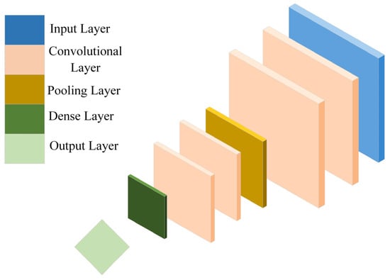
Figure 1. Typical convolutional neural network structure diagram.

The core modules of CNN are convolutional layers and pooling layers, which use alternating convolution and pooling operations to achieve layer-by-layer stripping of input data and mining of abstract features hidden in the data.

The convolutional layer is a feature extraction layer that performs convolution operations on input features to obtain a feature map. The convolution operation is represented as follows:

$${\mathbf{y}}_j^l=f({\displaystyle \sum _i{\mathit{w}}_{ij}^l{\mathit{x}}_i^{l-1}+{\mathit{b}}_i^l})$$

(1)

where b_i^l is the bias matrix; w_ij^l is the weight matrix; y_j^l is the convolutional layer feature of the l layer; x_i^l−1 is the i feature of the l − 1 layer; f is the activation function.

In order to better utilize deep learning models for mining relevant features after sparsity, it is common to connect the Relu (x) activation function after the convolutional layer to increase the nonlinearity of the model, allowing the neural network to approximate any nonlinear function arbitrarily. Relu (x) is represented as follows:

$$\mathrm{Relu}(x)=\left\{\begin{array}{cc}x& x>0\\ 0& x<0\end{array}\right\}$$

(2)

The pooling layer is a downsampling layer that aims to reduce the amount of data while maintaining feature-scale invariance. The pooling operation is represented as follows:

$${\mathit{x}}_j^l=f({\mathit{\beta }}_j^{l-1}down({\mathit{x}}_j^{l-1}+{\mathit{b}}_j^l))$$

(3)

β_j^l−1 is the weight matrix; b_j^l is the bias matrix; down is a downsampling function; x_j^l−1, x_j^l is the result before and after pooling.

2.2. Depthwise Separable Convolution

Depthwise Separable Convolution decomposes traditional convolution operations into two parts: Depthwise Convolution and Pointwise Convolution. Among them, channel-by-channel convolution is performed on each channel without changing the input feature depth, resulting in an output feature map with the same depth as the input feature map, as shown in Figure 2. Point-by-point convolution is the same as the traditional convolution operation, which uses a 1 × 1 convolution kernel to increase the dimensionality of the feature map, as shown in Figure 3. Taking a 3-channel color image with 5 × 5 pixels as an example, when performing depthwise separable convolution using 3 × 3 × 4 convolution kernels, the theoretical computational cost is 675 when convolving channel by channel; When convolving point by point, the theoretical computational cost is 3 × 4 × 5 × 5 = 300, and the total theoretical computational cost is 675 + 300 = 975. When using traditional convolution operations, the theoretical computational cost is 2700, which is about three times that of depthwise separable convolution. Therefore, when constructing lightweight fault diagnosis models, replacing traditional convolution operations with depthwise separable convolution can achieve fewer parameters and computational complexity.

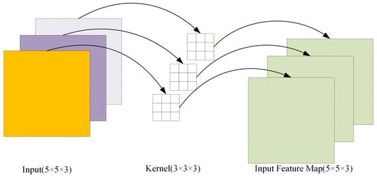
Figure 2. Depthwise convolution.

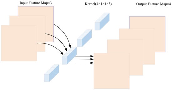
Figure 3. Pointwise convolution.

2.3. Model Optimization

2.3.1. MBConv Module and Fused-MBConv Module

The EfficientNet V2 network model was proposed by Tan et al. in April 2021 [26]. In the original Efficient V1 version, MBConv (Depthwise Separable Convolution) in shallow networks was replaced with Fused-MBConv, and NAS was used to search for the best combination. At the same time, the amplification factor of 1 × 1 convolution kernel in each module was reduced to form a faster and smaller convolutional neural network model, which can effectively reduce parameters and improve the efficiency of model training. The MBConv module is shown in Figure 4.

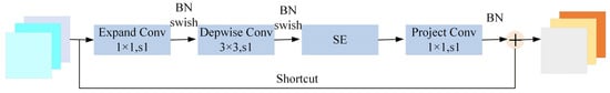
Figure 4. MBConv module.

The MBConv module is mainly composed of depthwise separable convolution and SE attention mechanism and adopts an inverse residual structure to reduce the information lost by high-dimensional features after passing through the activation function. The MBConv module first performs dimensionality enhancement on the input feature map through a 1 × 1 convolution kernel, then performs a depthwise separable convolution operation to reduce model parameters, and then uses the SE channel attention mechanism to highlight more important channel information. Finally, it performs dimensionality reduction through a 1 × 1 convolution kernel and adds shortcut connections to prevent gradient divergence. The model constructed in this article does not repeatedly stack the same MBConv and Fused-MBConv modules; therefore, the Dropout layer is removed.

Due to the fact that using the MBConv module in the shallow layers of the model did not accelerate the training speed, the Fused-MBConv module was proposed, which replaces the depthwise separable convolution in the MBConv module with the traditional 3 × 3 convolution, and then reduces the dimensionality through a 1 × 1 convolution kernel to improve the interaction of information between channels, as shown in Figure 5.

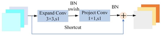
Figure 5. Fused-MBConv module.

2.3.2. Attention Mechanism

The core task of the attention mechanism is to select more critical feature information from many feature information. In recent years, it has become popular in various fields of deep learning. The application of this attention mechanism can be seen in various tasks such as natural language processing and image processing. The essence is to independently learn the importance of each channel through the network and give different weight coefficients to each output channel, so as to highlight important features and suppress unimportant features, making the bearing fault diagnosis of the model more accurate. The SE mechanism is shown in Figure 6. This method adds attention in the channel dimension. By means of automatic learning, it uses another new neural network to obtain the importance of each channel of the feature map. Then, it uses this importance to assign a weight value to each feature, thereby enabling the neural network to focus on certain feature channels and suppress irrelevant noise interference. It enhances the channels of the feature map that are useful for the current task and suppresses the channels that are less useful for the current task. This intrinsic mechanism provides potential advantages for the model’s stability in noisy environments.

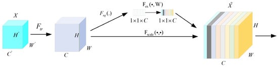
Figure 6. SE attention mechanism.

2.3.3. Inception Module

As a classic convolutional neural network model, InceptionNet is most characterized by the expansion of the convolutional operation in each layer of the neural network. The expanded convolutional layers conduct feature extraction and pooling operations at different scales, thereby acquiring feature information at multiple scales. Eventually, the feature information at various scales is integrated through a concatenation operation. The introduction of the InceptionNet network not only improves the classification performance of the network but also reduces the computational cost while maintaining the model quality. In this study, the InceptionV2 module is employed, where the 5 × 5 convolutional kernel in the convolutional layer is replaced by two 3 × 3 convolutional kernels, as specifically depicted in Figure 7.

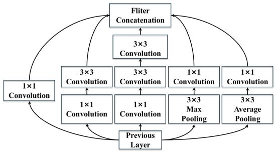
Figure 7. Improved Inception V2 module.

2.4. Training Optimization

2.4.1. Function of Activation

In order to improve the nonlinear expression ability of the neural network model, the neural network model can approach the nonlinear model, and the activation function is introduced to improve the expression ability of the network model. As shown in Figure 8, the most widely used activation function in neural network models is the Relu activation function shown in Equation (1). Although the calculation amount of the Relu activation function is small, it can effectively alleviate such problems as gradient loss, but when the value of the input activation function is negative, the neuron will be directly necrotic, causing the loss of this part of the feature information. The Swish activation function shown in Formula (2) has the characteristics of non-monotonicity, unsaturation, and smoothness compared with the Relu activation function, which can effectively solve the neuronecrosis caused by the Relu function.

$$f(x)=x\ast sigmoid(\beta x)$$

(4)

where β is a constant or a trainable parameter.

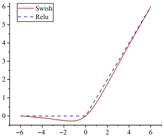
Figure 8. Swish and Relu activation function images.

2.4.2. Random Gradient Descent

Training of a neural network model is based on the gradient descent method, and calculating the gradient of each batch of data will cause slow training. The StoGradient Decline (SGD) optimizer selects one sample from each batch of samples to update the gradient, removes redundant calculation, supports online updates, makes the model have a faster training speed, effectively jumps out of the local optimal solution, and makes it easier to find the global optimal solution corresponding to the loss function.

3. Multi-Scale Convolution Feature Fusion Model Architecture

3.1. Model Structure

The EfficientNet V2 model achieves faster training speed, higher accuracy, fewer parameters, and reduced theoretical computational load in image classification tasks by combining MBConv and Fused-MBconv modules, demonstrating superior performance. However, two challenges arise in addressing rolling bearing fault diagnosis: first, the lack of sufficient rolling bearing vibration signal data to train the network for accurate fault diagnosis models; second, complex network structures not only increase computational load but also risk overfitting in data-limited scenarios, failing to meet expected performance. To address this, the Inception module was improved by integrating depthwise separable convolution to fuse multi-scale convolutional features, resulting in more compact and lightweight feature extraction modules—Inception1 and Inception2, as illustrated in Figure 9 and Figure 10.

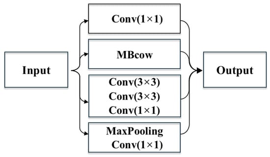
Figure 9. Inception1 architecture.

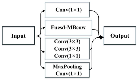
Figure 10. Inception2 architecture.

The multi-scale convolution model constructed in this study first performs feature extraction on the input through two sets of convolutional layers and then reduces the feature dimension through the Max pooling method to extract the main feature information. Then, through Inception1 and 2 modules, feature extraction and pooling at different scales are carried out. Subsequently, through the SE attention mechanism, the information of each channel is learned to obtain the weight coefficients between channels, thereby further extracting the main features. Then, by utilizing the Inception3 and 4 modules, mainly based on depthwise separable convolution, high-dimensional features are extracted while reducing the number of computational parameters. Finally, the high-dimensional features are compressed and aggregated through the global average pooling layer, converting the feature mapping into a fixed-dimensional vector representation. Subsequently, a fully connected layer is added to deeply integrate and perform nonlinear transformation on this vector feature, further enhancing the discrimination of key fault features and screening redundant information. Finally, the fault diagnosis type of the bearing is obtained through the SoftMax classifier. The detailed network architecture is illustrated in Figure 11.

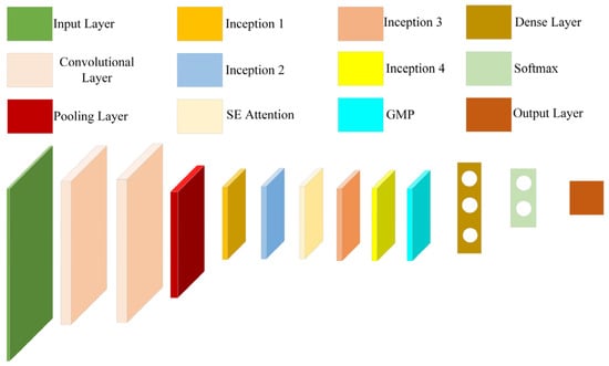
Figure 11. Network structure diagram.

3.2. Fault Diagnosis Process

The training flow of the network is shown in Figure 12. The training process of the network is as follows:

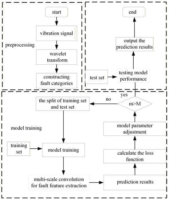
Figure 12. Fault diagnosis flow chart.

(1)

Generate a time–frequency diagram of an original vibration signal by means of a discrete wavelet transform;

(2)

Construct the corresponding fault category of the bearing time–frequency diagram through the unique heat code;

(3)

Divide the data into a training set and a test set;

(4)

Input the training set data into a multi-scale convolution network for training, and extract the fault characteristics of a rolling bearing;

(5)

Classify the fault category of the bearing using the soft max classifier;

(6)

Calculate the loss function using cross-entropy;

(7)

Update the parameters of the model by the loss function and the gradient descent method; complete the training of the model when the iteration number m of the network reaches N, otherwise repeat steps (4) to (6);

(8)

Test the performance of the trained model on the test set; output the calculation results and end the process.

4. Experiment

In order to verify the accuracy and generalization of the proposed rolling bearing failure diagnosis model, the Xi’an Jiaotong University bearing data set (XJTU-SY) and the University of Case Western Reserve Bearing data set (CWRU) were tested.

4.1. Case Western Reserve Bearing Data Set

4.1.1. Data Set Introduction and Processing

To verify the validity of the fault diagnosis model under single load and variable load, tests were conducted using the Case Western Reserve Bearing Data Set (CWRU), the test bearing model is SKF6205, and the parameters of the bearing are shown in Table 1.

Table 1. SKF6205 bearing parameters.

Test Bearing	Inner Ring Diameter (mm)	Outer Ring Diameter (mm)	Rolling Element Diameter (mm)	Number of Rollers (Per)	Pitch Diameter (mm)
SKF6205	25	52	7.94	9	39.04

This data set adopts electric spark machining technology, and single-point faults with diameters of 0.1778 mm, 0.3556 mm, and 0.5334 mm are generated by manual machining at three parts of the bearing outer ring, inner ring, and rolling elements, and tests are conducted under load conditions of 0, 1, 2, and 3 HP motors, respectively. The vibration acceleration signal of the faulty bearing is collected by the acceleration sensor. In this experiment, the fault data of the outer ring, inner ring, and rolling body under three load working conditions of 0, 1, and 2 horsepower are taken. The fault of the damage point of the outer ring at 6 o’clock is selected. The division of the experimental data set is shown in Table 2.

Table 2. Data set partitioning.

Data Tag	Damage Diameter (mm)	Location of Damage	Number of Training Set Samples	Number of Verification Set Samples	Number of Test Set Samples
1	0.1778	Bearing inner race	800	100	100
2		Bearing outer race	800	100	100
3		Rolling elements	800	100	100
4	0.3556	Bearing inner race	800	100	100
5		Bearing outer race	800	100	100
6		Rolling elements	800	100	100
7	0.5334	Bearing inner race	800	100	100
8		Bearing outer race	800	100	100
9		Rolling elements	800	100	100
10	Normal	Nothing	800	100	100

In this experiment, the bearing data at the driving end is adopted, and the sampling frequency is 48 kHz. According to different parts of the bearing and the varying degrees of single-point damage at each bearing part, a total of 10 types of states are set according to different parts of the bearing and different degrees of single-point damage at each bearing part. Each type of state is subject to continuous wavelet transformation. A total of 4000 training set samples, 500 verification set samples, and 500 test set samples are set according to the ratio of 8:1:1. At the same time, in order to avoid overfitting, the input images are randomly turned over, randomly cut, and mirror turned over. Time-domain images of a bearing with a damage diameter of 0.1778 mm at 0 horsepower are shown in Figure 13 and Figure 14.

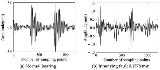
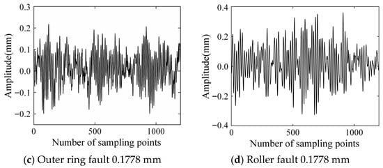
Figure 13. Time-domain diagram of partial bearing state.

Figure 14. Time–frequency diagram of partial bearing state.

4.1.2. Comparison and Analysis of Fault Diagnosis Results

The model is programmed in the Tennorflow2.4 in-depth learning framework under Window10 system. The initial learning rate of the SGD optimizer is set to 0.01, the momentum parameter to 0.9, and the batch training size to 32 by adjusting the image to 224 × 224 as input.

The experimental results of the model are shown in Figure 15. From the analysis in the figure, it can be seen that this method can effectively extract the bearing failure characteristics under a single load, achieving 100% accuracy.

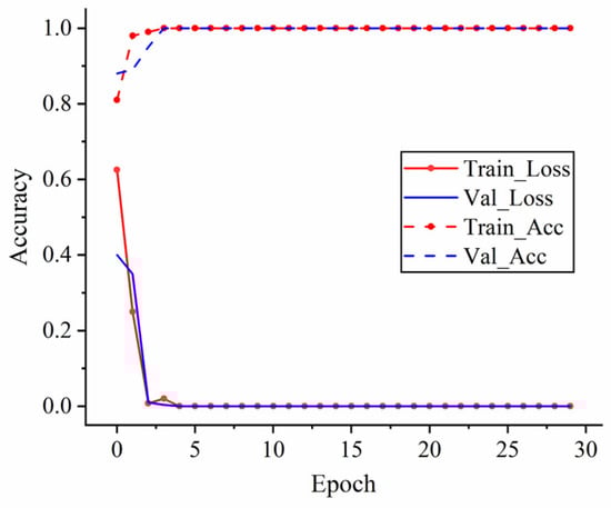
Figure 15. Zero load data set experimental results.

4.1.3. Variable Load Fault Diagnosis Result Analysis

In actual engineering practice, the running environment of rolling bearings is often complicated, and rolling bearings in operation will bear different loads. In order to further verify the accuracy and generalization of the fault diagnosis of the model under different load conditions, the bearing data with loads of 1, 2, and 3 horsepower in the University of Chase bearing data are selected to train the model, respectively, and then the trained model of each horsepower is tested with the data sets of the other two horsepower. At the same time, the artificial feature + SVM experiment results and the ECA-CNN experiment results reported in the literature [27], and the bearing fault diagnosis method of IDCNN in the literature [28], are introduced for the comparative experiment. The experiment results are shown in Table 3.

Table 3. Variable load-bearing data set test results.

Model Name	Horse-Power → 2 Horse-Power	Horse-Power → 3 Horse-Power	2 Horse-Power → Horse-Power	2 Horse-Power → 3 Horse-Power	3 Horse-Power → Horse-Power	3 Horse-Power → 2 Horse-Power	Average Value
Artificial feature + SVM	86.8	71.8	82.8	79.4	63.8	77.8	77.1
1DCNN	95.6	91.2	94.0	96.8	90.0	91.2	93.1
ECA-CNN	99.1	98.0	92.3	95.6	97.7	86.2	94.8
MAWPN	98.4	97.6	91.8	96.4	95.6	90.8	95.1
LSTM	98.6	97.8	92.1	95.8	96.4	91.2	95.3
Method in this study	99.1	99.1	99.6	99.1	96.8	86.6	96.7

It can be seen from Table 3 that the method of manual feature extraction and SVM classifier has poor generalization and weak adaptability under different load conditions; the fault diagnosis model based on a one-dimensional convolutional neural network (1DCNN) has a low recognition rate of fault diagnosis under different load conditions; the convolutional neural network introduced with attention mechanism of ECA can obtain the weight coefficient between different channels, and has good fault diagnosis identification rate under different load conditions. MAWPN and LSTM methods: Both types of methods exhibit strong feature extraction capabilities under variable load conditions, with excellent model adaptive performance, and can well adapt to the fluctuations in the diagnostic environment caused by load changes. However, both have common flaws—they fail to allocate differentiated weights for the importance of different features, which leads to room for improvement in the fault diagnosis rate and fails to fully unleash the performance potential of the model.

4.2. XJTU-SY Bearing Data Set

4.2.1. Data Set Introduction and Processing

The bearing data set [29] published by Xi’an Jiaotong University is used to verify the fault diagnosis results of different types of bearings. The test bearing model is the LDK UER204 rolling bearing. The test platform is shown in Figure 16, mainly composed of an AC motor, a digital force display, a rotating shaft, a support bearing, a test bearing, etc. The radial force can be adjusted by the hydraulic loading system, and the AC motor can adjust the speed to set different working conditions. There are three kinds of working conditions in the experiment, five bearings for each kind of working condition, and the vibration signal is collected by the dynamic signal collector. The sampling interval is 1 min, the sampling frequency is 25.6 kHz, and the single sampling time is 1.28 s.

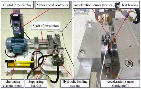
Figure 16. Experimental platform.

In this experiment, five types of bearing vibration signals are selected from the three types of working conditions as the test objects, including four types of fault characteristics, i.e., inner ring wear, outer ring wear, outer ring fracture and overall bearing failure, and normal bearing, as shown in Figure 17.

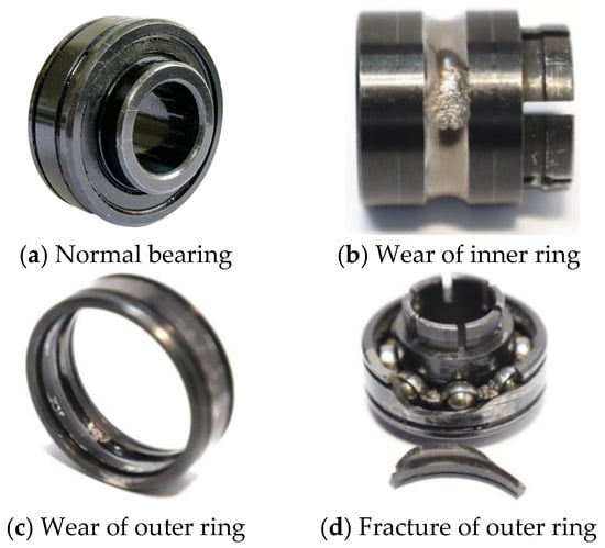
Figure 17. Failure position of normal bearing and failed bearing.

4.2.2. Analysis of Fault Diagnosis Results

The structure of this experimental model is the same as before, and the model parameters are adopted. The experimental results are shown in Figure 18.

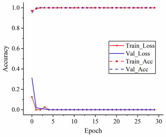
Figure 18. Test results of bearing data set of XJTU-SY.

In order to further verify the stability of the model, the model was repeated 10 times, and the experimental results are shown in Table 4. The results show that the proposed model can quickly converge, has good stability, and can accurately distinguish different bearing faults, so it is more suitable to be applied in engineering practice in cases with limited data.

Table 4. Repetition test results.

Experiment No	1	2	3	4	5	6	7	8	9	10
Accuracy rate (%)	100	100	100	100	100	100	100	100	100	100
Average training time (s)	168	169	167	161	165	165	165	164	165	166

5. Conclusions

This study presents an improved multi-scale convolutional feature fusion model for rolling bearing fault diagnosis based on the Inception module. The original vibration signal is generated into a time–frequency diagram through continuous wavelet transform, and a data set is constructed according to the scale as the input of the fault diagnosis model. The bearing data set of Xi’an Jiaotong University and the bearing data set of Case Western Reserve University are respectively used for verification.

(1)

The model can automatically extract different features from the time–frequency diagram, reduce the requirements of manual bearing fault diagnosis, and accurately classify different bearing faults.

(2)

The model has good universality in different bearing data sets and can maintain a high accuracy rate of fault identification under variable load conditions.

(3)

By reducing the training parameters, accelerating the model training speed, and ensuring the model has good performance at the same time, this has a good application prospect in practical engineering. Fault diagnosis through mobile terminals will be the focus of future research.

(4)

This study focused on the structures of MBConv, fused MBConv, SE attention mechanism, and Inception module, quantitatively evaluated their noise robustness under signal-to-noise ratio conditions, and conducted ablation experiments and noise recognition for different models as important research directions in the future.

References

- Gui, S.; Zou, N.; Li, N. Development Plans for Artificial Intelligence in Foreign Military Fields and the Application of Ship Intelligence Technologies. Ship Sci. Technol. 2020, 42, 174–177. [Google Scholar] [CrossRef]
- Yao, Y. Data-Driven and Neural Network-Based Fault Prediction for Ship Mechanical Bearings. Nav. Sci. Technol. 2023, 45, 119–122. [Google Scholar] [CrossRef]
- Hu, C. Intelligent Health Management Technology for Equipment. J. Intell. Syst. 2023, 18, 1142. [Google Scholar] [CrossRef]
- Althubaiti, A.; Elasha, F.; Teixeira, J. Fault diagnosis and health management of bearings in rotating equipment based on vibration analysis–a review. J. Vibroeng. 2022, 24, 46–74. [Google Scholar] [CrossRef]
- Yao, Q.; Bie, S.; Yu, J.; Chen, Q. A Bearing Fault Diagnosis Method Combining an Improved Inception V2 Module and CBAM. J. Vib. Eng. 2022, 35, 949–957. [Google Scholar] [CrossRef]
- Shi, J.; Pan, H.; Cheng, J.; Zheng, J.; Liu, X. A fault diagnosis approach for roller bearing based on boundary smooth support matrix machine. Meas. Sci. Technol. 2023, 35, 025138. [Google Scholar] [CrossRef]
- Huang, W.; Cheng, J.; Yang, Y.; Guo, G. An Improved Deep Convolutional Neural Network with Multi-scale Information for Bearing Fault Diagnosis. Neurocomputing 2019, 359, 77–92. [Google Scholar] [CrossRef]
- Zhao, B.; Zhang, X.; Zhan, Z.; Pang, S. Deep Multi-Scale Convolutional Transfer Learning Network: A Novel Method for Intelligent Fault Diagnosis of Rolling Bearings under Variable Working Conditions and Domains. Neurocomputing 2020, 407, 24–38. [Google Scholar] [CrossRef]
- Chen, X.; Zhang, B.; Gao, D. Bearing Fault Diagnosis Base on Multi-Scale CNN and LSTM Model. J. Intell. Manuf. 2021, 32, 971–987. [Google Scholar] [CrossRef]
- Jin, Y.; Qin, C.; Zhang, Z.; Tao, J.; Liu, C. A Multi-Scale Convolutional Neural Network for Bearing Compound Fault Diagnosis under Various Noise Conditions. Sci. China Technol. Sci. 2022, 65, 2551–2563. [Google Scholar] [CrossRef]
- Shang, Z.; Li, W.; Gao, M.; Liu, X.; Yu, Y. An Intelligent Fault Diagnosis Method of Multi-Scale Deep Feature Fusion Based on Information Entropy. Chin. J. Mech. Eng. 2021, 34, 58. [Google Scholar] [CrossRef]
- Wang, Y.; Liang, J.; Gu, X.; Ling, D.; Yu, H. Multi-scale Attention Mechanism Residual Neural Network for Fault Diagnosis of Rolling Bearings. Proc. Inst. Mech. Eng. Part C J. Mech. Eng. Sci. 2022, 236, 10615–10629. [Google Scholar] [CrossRef]
- Guan, P.; Zhang, T.; Zhou, L. RUL Prediction of Rolling Bearings Based on Multi-Information Fusion and Autoencoder Modeling. Processes 2024, 12, 1831. [Google Scholar] [CrossRef]
- Tang, X.; He, Q.; Gu, X.; Li, C.; Zhang, H.; Lu, J. A Novel Bearing Fault Diagnosis Method Based on GL-mRMR-SVM. Processes 2020, 8, 784. [Google Scholar] [CrossRef]
- Li, Q. New sparse regularization approach for extracting transient impulses from fault vibration signal of rotating machinery. Mech. Syst. Signal Process. 2024, 209, 111101. [Google Scholar] [CrossRef]
- Zhou, Z. Diagnostic Methods for Outer Ring Failures in Shipboard Electric Motor Bearings. Nav. Sci. Technol. 2023, 45, 128–131. [Google Scholar] [CrossRef]
- Yu, J.; Shao, J.; Peng, X.; Liu, T.; Yao, Q. Remaining Useful Life of the Rolling Bearings Prediction Method Based on Transfer Learning Integrated with CNN-GRU-MHA. Appl. Sci 2024, 14, 9039. [Google Scholar] [CrossRef]
- Yang, Y.; Zhang, N.; Cheng, J. Application of Fully Parametric Dynamic Learning Deep Belief Networks in Rolling Bearing Life Prediction. Vib. Shock. 2019, 38, 199–205+249. [Google Scholar] [CrossRef]
- Xue, Y.; Shen, N.; Dou, D. Diagnosis of Rolling Bearing Fault Severity Based on One-Dimensional Convolutional Neural Networks. Bearing 2021, 48–54. [Google Scholar] [CrossRef]
- Hu, X.; Jing, Y.; Song, Z.; Hou, Y. Research on Bearing Fault Identification Using Deep Convolutional Neural Networks Based on CNN-SVM. Vib. Shock. 2019, 38, 173–178. [Google Scholar] [CrossRef]
- Zhou, Q.; Chai, B.; Tang, C.; Guo, Y.; Wang, K.; Wu, W.; Cao, B.; Ye, Y. Enhancing multimodal fault diagnosis in mechanical systems via mixture of experts. Complex Intell. Syst. 2025, 11, 425. [Google Scholar] [CrossRef]
- Zhou, Q.; Chai, B.; Tang, C.; Guo, Y.; Wang, K.; Nie, X.; Ye, Y. Enhanced YOLOv8 with DWR-DRB and SPD-Conv for Mechanical Wear Fault Diagnosis in Aero-Engines. Sensors 2025, 25, 5294. [Google Scholar] [CrossRef] [PubMed]
- Zhou, Q.; Chai, B.; Guo, Y.; Li, T.; Zhou, S.; Wang, K.; Ye, Y. Multimodal mechanical wear fault diagnosis: Fusion of signal characterization and image information. Results Eng. 2025, 28, 107204. [Google Scholar] [CrossRef]
- Yuan, L.; Chen, Y.; Du, B.; Zhang, Z.; Liu, G. Research on Rolling Bearing Fault Diagnosis Based on AlexNet and Transfer Learning. Electromech. Eng. 2021, 38, 1016–1022. [Google Scholar] [CrossRef]
- Zhang, X.; Liu, S.; Yu, D.; Lei, J.; Li, L. Improved Deep Convolutional Neural Network and Its Application in Fault Diagnosis of Rolling Bearings Under Variable Operating Conditions. J. Xi’an Jiaotong Univ. 2021, 55, 1–8. [Google Scholar] [CrossRef]
- Tan, M.; Le, Q. EfficientNetV2: Smaller Models and Faster Training. arXiv 2021, arXiv:2104.00298. [Google Scholar]
- Xie, T.; Dong, S. Fault Diagnosis Method for Rolling Bearings Under Noise and Variable Load Conditions Based on an Improved CNN. Noise Vib. Control. 2021, 41, 111–117. [Google Scholar] [CrossRef]
- Feng, L.; Xu, J.; Tian, R.; Jiao, L.; Li, T. Research on Bearing Fault Diagnosis Method Based on One-Dimensional Convolutional Neural Network. Heavy Mach. 2021, 57–62. [Google Scholar] [CrossRef]
- Wang, B.; Lei, Y.; Li, N.; Li, N. A Hybrid Prognostics Approach for Estimating Remaining Useful Life of Rolling Element Bearings. IEEE Trans. Reliab. 2020, 69, 401–412. [Google Scholar] [CrossRef]
Disclaimer/Publisher’s Note: The statements, opinions and data contained in all publications are solely those of the individual author(s) and contributor(s) and not of MDPI and/or the editor(s). MDPI and/or the editor(s) disclaim responsibility for any injury to people or property resulting from any ideas, methods, instructions or products referred to in the content. |
© 2025 by the authors. Licensee MDPI, Basel, Switzerland. This article is an open access article distributed under the terms and conditions of the Creative Commons Attribution (CC BY) license (https://creativecommons.org/licenses/by/4.0/).