Abstract
Conglomerate reservoirs often exhibit chaotic internal structures and strong heterogeneity due to the influence of gravel, which seriously restricts the balanced initiation of multiple clusters and the balanced expansion of artificial fractures in the volume fracturing section of horizontal wells. Therefore, clarifying the distribution pattern of gravel in conglomerate reservoirs is of great significance for the design and parameter optimization of horizontal well segmentation and clustering. This work conducts research on the interpretation results of imaging logging, establishes a characterization model for the distribution characteristics of gravel around horizontal wells, develops gravel feature recognition and analysis software for conglomerate reservoirs using image processing technology, and effectively obtains the morphology of gravel in imaging logging. Based on this, a correlation model between conventional logging and imaging logging is constructed to predict the distribution of gravel in horizontal wells without imaging logging. Using the Kriging interpolation method, a “point line surface” gravel distribution prediction method is proposed. Through three methods of imaging logging, downhole eagle-eye camera, and on-site coring, the model accuracy is found to be greater than 80%, guiding segmented clustering to avoid high gravel areas. During the fracturing process, the wellhead pressure is lower than that of adjacent wells, enabling greater fluid savings per well. The production effect is better than that of adjacent wells in the same block, providing a reference for the study of gravel distribution characteristics in conglomerate oil reservoirs.
1. Introduction
As the global economy continues to develop, society’s demand for petroleum energy keeps rising, with the pressure on the supply–demand balance becoming increasingly apparent. Within global oil reserves, conventional reservoirs account for 30%, while unconventional reservoirs constitute 70%. It is generally acknowledged that most easily accessible reservoirs have begun exhibiting a decline in conventional oil production [1,2]. To meet the growing demand for petroleum, researchers will not only enhance oil recovery rates in existing fields but also develop new unconventional energy resources. Conglomerate reservoirs represent a typical type of coarse-grained sedimentary unconventional reservoir [3]. Following the initial discovery of multiple sandstone and conglomerate reservoirs in the Triassic Tupungato oil field and Jurassic–Cretaceous strata of Argentina’s Cuyo Basin [4], similar reservoirs have since been identified in countries including the United States, Canada, Brazil, and the United Kingdom [5,6]. Domestically, effective utilization of conglomerate reservoirs has been achieved in regions such as the Mahu Depression in Xinjiang, the western depression of the Liaohe Oilfield, and the Erlian Basin of the Shengli Oilfield. Among these, the Mahu tight conglomerate reservoir—China’s largest integrated conglomerate reservoir—has evolved over more than a decade of development into an annual production base yielding 3 million tons of unconventional oil. The development of gravel-packed reservoirs represents an iterative process of practice-based learning, progressing through stages including water injection development, horizontal well volume fracturing, intra-stage multi-cluster dense cutting, intra-stage multi-cluster temporary plug fracturing, three-dimensional well network fracturing, and pre-injection carbon dioxide fracturing for enhanced production. Both laboratory experiments and field practice indicate significant differences in mineral composition and rock mechanical properties between gravel and matrix within the reservoir [7]. This results in pronounced heterogeneity, where injected water during waterflooding tends to flow along the gravel–matrix–cementation interface, leading to premature waterflooding of oil wells. During horizontal well fracturing, artificial fractures exhibit two modes at gravel zones: penetration through gravel and bypassing gravel [8]. Post-fracturing downhole Eagle-Eye monitoring revealed low uniformity in fracture initiation across clusters within gravel sections, with some near-base perforation clusters receiving over 70% of the proppant load for that section [9]. Therefore, clarifying the gravel content and distribution patterns in gravel reservoirs is crucial for achieving uniform fracture initiation across multiple clusters within fractured sections and optimizing fracture parameters.
Predictions of gravel distribution characteristics currently rely primarily on sedimentary facies analysis, seismic attribute analysis, and well log curve feature inversion. These methods leverage differences in wave impedance and well log data between gravel and matrix to predict gravel content and size through differential characteristics. The fan delta foreland, fan delta plain, and pre-fan delta have been divided into nine distinct conglomerate facies based on sedimentary genesis, sedimentary structure, grain shape, arrangement patterns, support forms, cementation types, and other characteristics; based on sedimentary structures, grain shape, arrangement patterns, support forms, and cementation types, nine conglomerate facies have been further defined [10]. High-velocity conglomerates induce abnormally elevated overlay velocities below the conglomerate extinction point by investigating gravel’s impact on underlying stratigraphic overlay velocities, enabling gravel-rich zone identification through these anomalies [11]. Five distinct seismic facies patterns have been listed for sandstone–conglomerate complexes based on the principle that sedimentary types dictate differing seismic facies characteristics [12]. Resistivity cutoff values have been proposed through core calibration based on resistivity differences in rock components within gravel reservoir electrical imaging [13]. Researchers have developed calculation methods for gravel, sandy, and muddy content, along with a grain size analysis method using pseudo-grain size probability cumulative curves, and others identified the characteristics of gravel and sandstone formations in the Kuche area of Tarim as low sonic velocity, high density, high resistivity, and low neutron content [14,15]. This was achieved by utilizing the principle that resistivity logging anomalies in gravel and sandstone strata correspond to high-resistivity anomalies and that the curve morphology is related to factors such as water influx and outflow cycles during deposition, distance from the source area, supply rate, flow energy, and sedimentary background. Logging curves of gravel reservoirs in the Yanjia-22 block have been characterized as exhibiting high gamma, medium-to-high natural potential, medium-to-low density, medium-to-low borehole diameter, and medium-to-low sonic characteristics [16]. Based on logging research, a quantitative calculation method was developed for gravel grain size using micro-resistivity imaging logging (MIRL) images [17]. By integrating digital image processing techniques, this approach established a method for calculating gravel grain size. Watershed algorithms were also introduced to investigate gravel identification within imaging logging images [18]. They enhanced the algorithm by adding filters, gradient processing, and region of interest (ROI) marking, thereby resolving the excessive segmentation issues inherent in watershed algorithms based on topological theory and simulated topography. Recently, a method was proposed for automatic identification and parameter calculation of gravel in electrical imaging based on a Saliency Object Detection Network [19,20,21,22,23,24,25,26,27]. This approach accurately calculates quantitative evaluation parameters such as grain size, roundness, and quantity using the identified gravel results. Seismic attribute analysis primarily relies on variations in wave impedance to infer gravel distribution. However, the complexity and heterogeneity of conglomerate reservoirs often cause wave impedance variations to be influenced by multiple factors, such as depositional environments and tectonic movements. This leads to potential errors in seismic data during the inversion process, thereby affecting the accuracy of gravel distribution predictions. Resistivity logging technology infers rock composition by measuring formation resistivity, but its accuracy is affected by multiple factors, including rock porosity, saturation, and fluid type. In conglomerate reservoirs, resistivity variations may not directly reflect gravel content and size, leading to imprecise quantitative assessments of gravel distribution. Furthermore, resistivity logging typically provides only local information, making comprehensive regional-scale predictions challenging.
In summary, while sediment facies analysis and seismic attribute analysis can yield gravel information, most approaches rely on inversion for prediction and cannot achieve a precise quantitative assessment. Logging-on-the-hole (LOH) feature analysis can capture continuous profile variations in gravel content along the wellbore axis, but no quantitative interpretation model linking LOH features to gravel content and size has been established [28,29,30,31,32,33,34,35]. Imaging logging currently represents the primary method for quantitative characterization of content and size [36,37,38,39,40,41]. However, it heavily relies on imaging logs, and quantitative calibration remains unattainable without such logs. Furthermore, imaging logging can only establish distribution characteristics on a single-well profile, failing to predict regional gravel content and size distribution [42,43,44,45,46,47,48,49,50]. Previous studies often failed to adequately account for the complexity of geological settings, such as variations in sedimentary facies and the influence of tectonic movements. The impact of these factors on gravel distribution may have been overlooked, leading to biased research outcomes. Many investigations employed a single methodology for analyzing gravel distribution, lacking a comprehensive approach. Integrating multiple data sources and analytical techniques could more effectively reveal the distribution characteristics of gravel.
To this end, building on the aforementioned research, this paper fully utilizes imaging logging interpretation results to establish a model that characterizes gravel distribution features around horizontal wells. It identifies two key parameters to represent gravel characteristics and employs image processing techniques to develop a method for characterizing the axial gravel distribution features based on imaging logging. To overcome the challenge of predicting distribution characteristics without imaging logs, a multivariate regression method is used to construct a correlation model between conventional logging and imaging logging. This enables the prediction of gravel distribution in horizontal wells without the need for imaging logs. The results are validated through three approaches, demonstrating high consistency. Building on this, a regional gravel distribution prediction method was developed using single-well prediction results, providing a basis for segmented and clustered optimization of conglomerate reservoirs and differentiated design of fracturing parameters.
2. Establishment of the Model for Characterizing the Distribution Characteristics of Gravel Around Wells
For sedimentary reservoirs formed by rapid accumulation of multi-phase alluvial fans, conglomerate reservoirs often exhibit complex internal structures and strong heterogeneity. During drilling in conglomerate reservoirs, horizontal wells frequently encounter multiple zones with varying gravel sizes and concentrations. To precisely characterize gravel distribution along the wellbore axis, consider an infinitesimal segment dx along the wellbore axis, as illustrated in Figure 1. When this infinitesimal element is sectioned axially, it forms a rectangle. The gravel radius and gravel density are defined on this rectangular infinitesimal element:
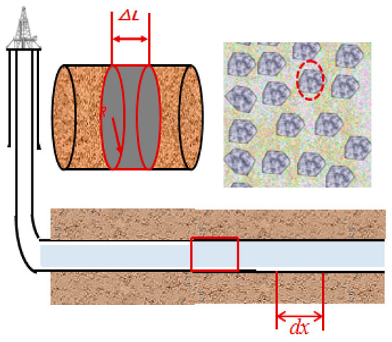
Figure 1.
Rectangular Microelement Representation of Gravel Linear Density and Radius.
Due to variations in the size and shape of gravel particles within the micro-element rectangle, a uniform numerical value cannot be used for characterization. To achieve quantitative representation of gravel size, the area of gravel particles with different shapes is calibrated via imaging logging. The gravel radius within the micro-element rectangle is then characterized using an equivalent circle approach, with the specific formula shown below:
In the formula, r denotes the radius of gravel on the infinitesimal rectangular body, mm, and A denotes the area of gravel calibrated on the infinitesimal rectangular body, mm2.
To quantitatively characterize the gravel content along the axial direction of a horizontal wellbore, the gravel linear density is defined as the gravel content per unit area along the wellbore axis. The specific formula is as follows:
In the formula, C represents the linear density of gravel along the borehole axis, units: pcs/m2; N denotes the gravel content within the rectangular element, units: pcs; R is the borehole radius, units: mm; and L is the length of the element, units: mm.
3. Method for Assessing Gravel Distribution Characteristics
3.1. Method for Characterizing Axial Gravel Distribution in Boreholes Based on Imaging Logging
FMI imaging logging employs an electrode array to perform array scanning or rotary scanning around the wellbore to measure electrical conductivity. The acquired conductivity data undergoes depth correction, velocity correction, and balancing to generate a two-dimensional resistivity image of the wellbore wall. In FMI imaging logging interpretations, subtle color variations represent changes in lithology and physical properties, with colors ranging from light to dark indicating decreasing conductivity values. Due to the poor conductivity of gravel in conglomerate reservoirs, it appears as blocky bright areas in electrical images, distinguishable from the background color of the imaging log. Therefore, gravel distribution characteristics can be extracted from the imaging log through image processing. Effective gravel information extraction is achieved through grayscale processing, blind zone filling, and image segmentation of the imaging log, as illustrated in Figure 2. The specific workflow comprises the following four steps:
① Grayscale processing is applied to the two-dimensional resistivity images from imaging logging. This conversion preserves overall and local chromatic brightness characteristics while transforming the image into grayscale, where brighter areas indicate potential gravel zones.
② Blind zone filling is applied to eliminate white band blind zones caused by electrode plate occlusion in imaging logging, neutralizing the influence of high conductivity at occlusion points.
③ Image segmentation techniques are applied to effectively extract bright regions from the filled image. Adaptive thresholding is used to isolate gravel from the image.
④ The convex hull algorithm is employed to sequentially extract the envelope areas of bright regions in the segmented imaging picture. This process statistically determines the radial and linear density distribution characteristics of gravel along the wellbore axis.

Figure 2.
Imaging Log Image Processing Workflow.
Figure 2.
Imaging Log Image Processing Workflow.

Based on the aforementioned principles, the “Conglomerate Reservoir Gravel Characteristic Identification and Analysis Software V1.0” was developed. This software enables automatic processing and interpretation of imaging logging data, exporting the processed and interpreted results in tabular format. The software interface is shown in Figure 3, and the computational results are presented in Figure 4.
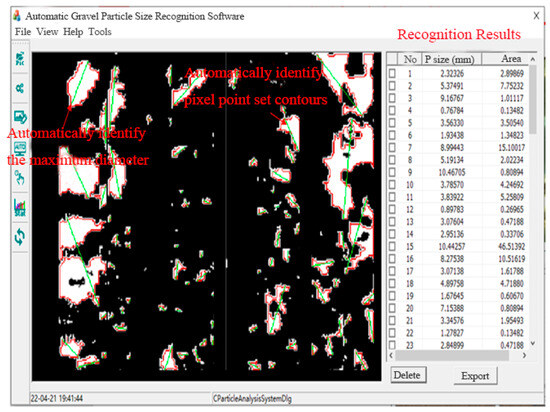
Figure 3.
Interface of the Gravel Characteristic Identification Analysis Software for Conglomerate Reservoirs.
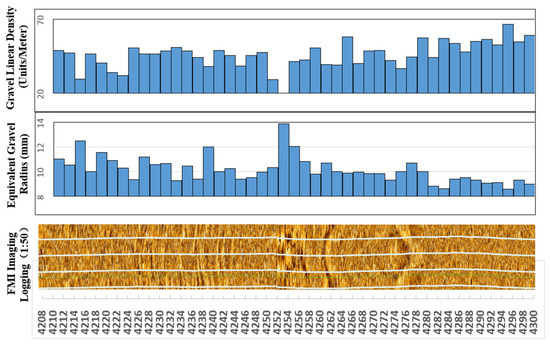
Figure 4.
JLX Well FMI Gravel Identification Results (4208–4300 m).
3.2. Method for Characterizing Axial Gravel Distribution in Boreholes Based on Logging Data
Considering the field operation cycle and costs, FMI imaging logging is not performed on every well. Therefore, it is necessary to establish correlations between conventional logging data and gravel distribution characteristics based on imaging logging interpretation results, thereby characterizing the gravel distribution around horizontal wells under conditions where imaging logging is unavailable. The p-value from statistics is introduced to characterize the association between different types of logging data and gravel linear density and content. The p-value is the probability of observing a test statistic at least as extreme as the current result under the assumption that the null hypothesis is true. In hypothesis testing, the p-value is compared to the significance level α: if p-value < α, the null hypothesis is rejected; otherwise, it is not rejected. Assume the null hypothesis is “There is no relationship between logging curve data and gravel equivalent radius or gravel linear density.” Set the significance level α = 0.1. If p-value < 0.1, reject the null hypothesis at the 0.1 significance level, indicating a statistically significant relationship exists between the logging curve and either the gravel equivalent radius or the gravel linear density. p-value analysis for the three indicators AC, CNL, and GR all yielded values less than 0.1. This indicates statistically significant relationships between these logging curves and gravel characteristics, as illustrated in Figure 5 and Figure 6.
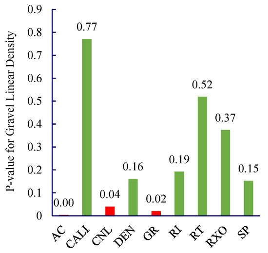
Figure 5.
Logging Curve and p-value of Gravel Line Density (4208–4264 m).
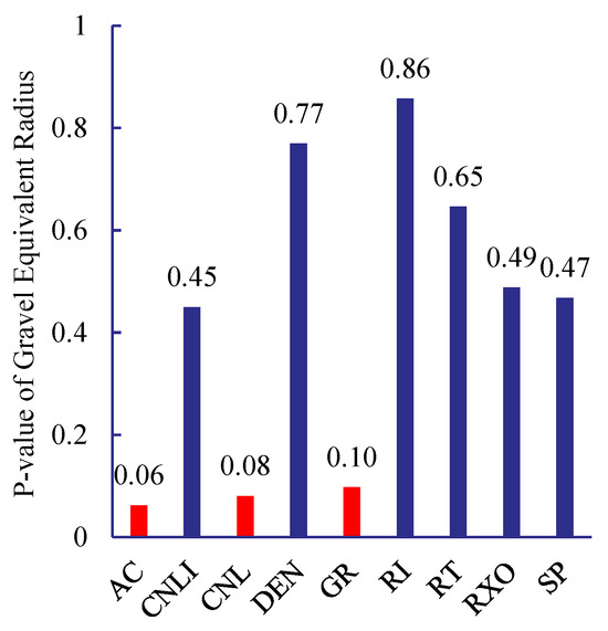
Figure 6.
Log Curves and p-Values for Gravel Equivalent Radius (4208–4264 m).
Using multiple regression analysis, predictive models were established for conventional logging curves in the fan area of the JL1 wellbore, relating to gravel equivalent radius and gravel line density, as shown in Equations (3) and (4). Linear regression was performed between the predicted and observed results, verifying a fitting accuracy exceeding 80%, as illustrated in Figure 7.
Equivalent Gravel Radius: r = −0.884AC − 1.44CNL + 0.694GR + 72.03
Gravel Linear Density: C = 0.152AC + 0.247CNL − 0.119GR + 5.64
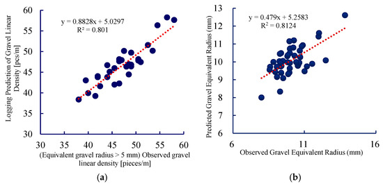
Figure 7.
Fitting Curve:(a) Gravel Linear Density; (b) Gravel Equivalent Radius.
3.3. Data Standardization and Regression Diagnostics
(1) Data Standardization
The purpose of data standardization is to eliminate the influence of different units and dimensions on regression coefficients, enabling variables to be compared on a uniform scale. This study employs zero-mean unit variance standardization (Z-score standardization):
Here, X represents the raw data, μ denotes the mean, and σ indicates the standard deviation.
(2) Regression Diagnosis
① R2 (determination coefficient):
R2 reflects the proportion of variance in the independent variable explained by the model, measuring the model’s ability to fit the data. Its value ranges from 0 to 1; a higher value indicates that the model better explains the variability in the data. The closer R2 is to 1, the more effectively the regression model predicts the dependent variable.
Among these, is the actual value, is the predicted value, and is the mean of the target variable.
② RMSE (Root Mean Square Error):
RMSE is a standard measure of regression model error, representing the average deviation between predicted and actual values. A smaller RMSE indicates higher prediction accuracy of the model.
Here, represents the actual value, and represents the predicted value.
③ Significance of the coefficient:
Significance tests for coefficients are used to assess whether independent variables have a significant effect on the dependent variable. A commonly used significance test is the t-test, whose test statistic is:
Here, represents the estimated regression coefficient, and the standard error indicates the uncertainty in the coefficient estimate. If the absolute value of the t-statistic is large and the corresponding p-value is less than the pre-set significance level of 0.1, then the independent variable is considered to have a significant effect on the dependent variable.
3.4. Regional Gravel Characteristic Distribution Characterization
To further characterize regional gravel distribution patterns, based on the axial gravel distribution in horizontal wells, Kriging interpolation was employed. Kriging interpolation is a spatial interpolation method grounded in geostatistics. It leverages the spatial autocorrelation of data by establishing a variogram model to quantify and describe the spatial structure of data, thereby providing an optimal, unbiased estimate for unknown points. Its core advantage lies not only in providing predicted values but also in offering the prediction error or uncertainty for each predicted point. This makes it a more scientific and accurate method than simple interpolation for reflecting the true spatial variation of geographic phenomena.
Kriging interpolation characterizes regional gravel line density and equivalent gravel radius size, providing a basis for depicting fracture propagation patterns in horizontal wells within conglomerate reservoirs. forming a “point-line-surface” gravel distribution prediction method, as shown in Figure 8a,b. The vertical axis represents horizontal section length, while the horizontal axis denotes lateral displacement. By determining the color of coordinate points based on the specified horizontal section length and lateral displacement, gravel line density and equivalent gravel radius can be predicted.
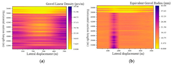
Figure 8.
Distribution Map:(a) Regional Gravel Line Density; (b) Regional Equivalent Gravel Radius.
4. Model Validation
To comprehensively evaluate the model’s generalization capability and predictive accuracy, this study employed three independent validation methods: imaging logging results, Eagle Eye test outcomes, and core sampling data. These approaches validated the model from distinct perspectives, ensuring its reliability in practical applications.
4.1. Imaging Logging Verification
The model accuracy was validated using gravel identification results from FMI imaging logging of the remaining sections of Well J1, as shown in Table 1.

Table 1.
Comparison of Gravel Equivalent Radius and Gravel Linear Density Identification Results.
Table 1 shows that for Well J1, the FMI observation indicates a gravel equivalent radius of 8–14 mm, while the logging model predicts a gravel equivalent radius of 9–12 mm, with an error range of 10–13% and an average error of 5.8%. The FMI-observed gravel linear density ranges from 20 to 60 grains per meter, while the logging model predicts a linear density of 20 to 60 grains per meter. The error ranges from 5% to 25%, with an average error of 12.8%. The standard errors for both predictions are relatively low, indicating that the coefficient estimates are more precise. The model-predicted parameter error is <15%, meeting engineering accuracy requirements.
4.2. Eagle-Eye Monitoring Results Comparison and Verification
The Downhole Eagle Eye is a high-precision downhole imaging technology. During model validation, it can serve as an independent verification data source, providing robust support for the accuracy and reliability of the model. Wells J2 and J1 are located within the same block. Through this model, the gravel equivalent radius and gravel linear density for Well J2 were obtained. Combined with Eagle Eye test results, single-stage gravel information (model prediction results) and annular erosion conditions (Eagle Eye test results) were derived, as shown in Table 2.
Table 2.
Single-Stage Gravel Information and Pore Erosion Conditions.
The heterogeneity of conglomerate reservoirs is characterized by the product of single-stage gravel line density variance and gravel equivalent radius variance. The reservoir heterogeneity is fitted with the average eroded aperture area from the Eagle Eye test, with the fitting results shown in Figure 9.
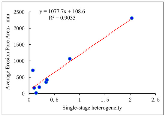
Figure 9.
Heterogeneity of Single-Segment Gravel and Pore Erosion Area.
As shown in Figure 9, the correlation between pore-eye erosion area and single-segment heterogeneity exceeds 90%, demonstrating that this model can accurately reflect the reservoir characteristics of conglomerate reservoirs.
4.3. Verification of Underground Core CT Scan Results
Core data represent the most direct method for model validation, providing authentic gravel parameters. Based on the conventional logging method for characterizing gravelly sandstone reservoirs developed in this study and utilizing gravel information from the CT images of Well M1 cores, As shown in Figure 10. A multiple linear regression analysis was conducted to clarify the relationship between gravel parameters and logging data: The equivalent gravel radius showed significant correlation with AC, GR, and RT in the logging curves, as shown in Figure 11 The linear density of gravel shows a strong correlation with CNL, DEN, and RT in the logging curves, as illustrated in Figure 12.
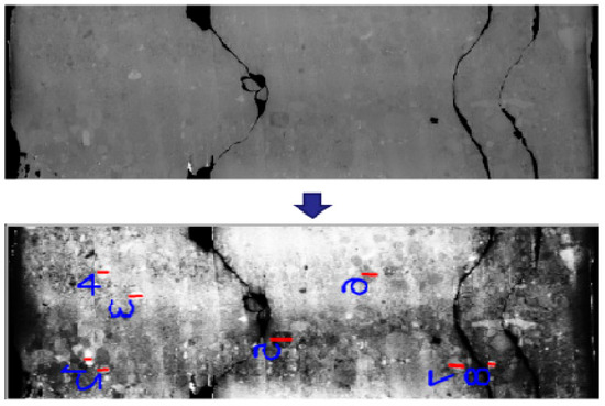
Figure 10.
Gravel Parameter Extraction from CT Images of Well M1.
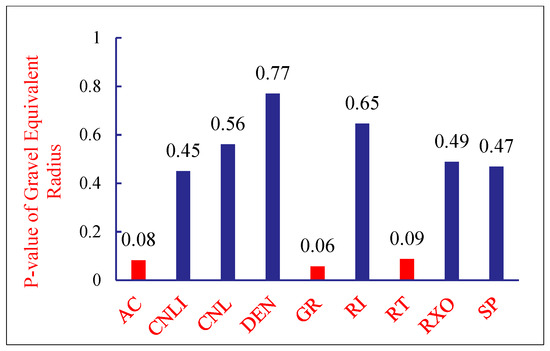
Figure 11.
Logging Curves and p-value of Gravel Equivalent Radius.
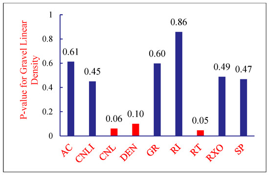
Figure 12.
Logging Curves and Gravel Line Density p-value.
The M1 curve and the equivalent radius and line density of gravel are modeled as shown in Formulas (5) and (6).
r = 0.173 × GR − 0.00497 × RT − 0.102 × AC + 1.33
C = 67.78 × DEN + 0.0742 × RT + 0.1298 × CNL − 161.414
Verification was conducted using CT scan results from core samples taken from Well M1, as shown in Figure 13.
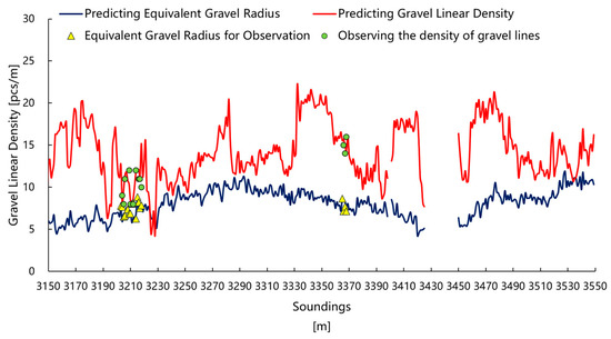
Figure 13.
Comparison of FMI Imaging Logging and Predicted Gravel Parameters.
The linear density model achieved an R2 value of 0.8135, while the equivalent conglomerate radius model attained an R2 of 0.7044, indicating both models effectively fit the data. The linear density model yielded an RMSE of 0.26, and the equivalent conglomerate radius model produced an RMSE of 0.21, signifying increasingly precise model predictions.
As shown in Figure 13, the gravel parameters predicted by this method exhibit minimal deviation (<10%) from the results obtained from core CT scans at Well M1. Possible causes for discrepancies between predicted and actual values include insufficient resolution of imaging logging images and physical changes in cored rock layers, demonstrating the method’s generalizability.
5. Field Application
During fracturing operations in conglomerate reservoirs, the presence of gravel fragments results in shorter perforation penetration depths compared to conventional sandstone formations, making fracturing more challenging. This often leads to difficulties in initiating fractures and To address this, the J2 well in a conglomerate reservoir employed the aforementioned method to precisely map gravel distribution along the wellbore axis. Fracturing design was segmented and clustered to avoid areas with high gravel density and large gravel radii, as illustrated in Figure 14.
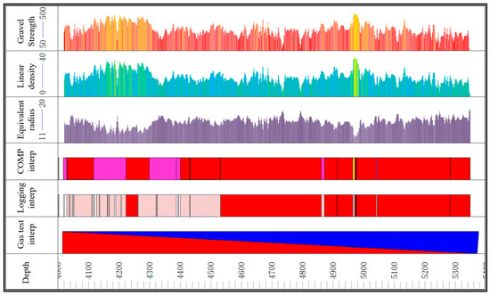
Figure 14.
Gravel Content and Segmented Clustering Results for the Horizontal Section of JL2 Well.
Well J2 employed horizontal well volume fracturing with a pumping rate of 12–14 m3/min. By avoiding areas with high gravel distribution, the operation difficulty was correspondingly lower. Sand injection was completed as designed, achieving a 10% fluid volume saving, as shown in Figure 15. The wellhead pressure was 3–5 MPa lower than that of adjacent wells, and the production performance exceeded that of neighboring wells in the block, as illustrated in Figure 16.
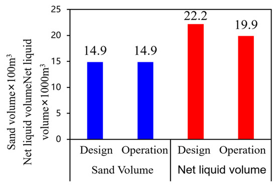
Figure 15.
Statistical Data on Fluid and Sand Volumes for JL2 Well.
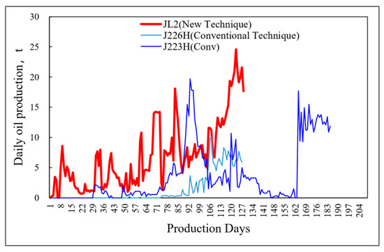
Figure 16.
Production comparison between Wells.
6. Conclusions
This study uniquely combines multiple methodologies to establish a gravel distribution characteristic model, develops image-processing-based identification software for precise recognition, and effectively predicts gravel distribution without imaging logging—all with high model accuracy. Emphasizing practical engineering applications, it reduces construction pressure, conserves fluid volume, and enhances production efficiency. Specific conclusions are as follows:
(1) A model for characterizing gravel distribution around horizontal wells was established to quantitatively describe the axial distribution of gravel content and size within wellbores. By systematically analyzing imaging log interpretation results and applying image processing techniques, gravel feature recognition software was developed, enabling effective extraction of gravel distribution characteristics from imaging logs and providing a robust basis for characterizing gravel in conglomerate reservoirs.
(2) The relationship between conventional logging curves and gravel content/size was clarified, leading to the establishment of a gravel distribution characterization method based on conventional logging data. Using Kriging interpolation, a “point-line-surface” approach for predicting gravel distribution was developed. Validation with imaging logging, downhole Eagle Eye data, and field coring confirmed model accuracy exceeding 80%.
(3) Detailed characterization of gravel distribution in horizontal wells guided staged and clustered fracturing operations, allowing bypass of high-gravel-content zones. This strategy effectively reduced fracturing complexity and lowered fracturing pressure by 3–5 MPa compared to neighboring wells. Single-well fluid consumption decreased by up to 10%, while production performance exceeded that of adjacent wells within the block. These findings provide a scientific basis for optimizing staged and clustered operations in gravel-rich reservoirs.
Based on existing research findings, future work can advance in multiple directions: the model accuracy requires improvement, so deep learning algorithms can be integrated to enhance gravel distribution prediction precision to over 90% [51,52,53]; beyond conglomerate reservoirs, the model can be extended to complex reservoir types, such as carbonates, to enhance applicability; real-time monitoring systems can be developed to optimize dynamic fracturing parameters; and green fracturing technologies can be explored to further reduce fluid consumption and environmental impact. These advancements will collectively drive the intelligent and sustainable development of oil and gas extraction.
Author Contributions
Investigation, Z.L., J.X., T.L., P.L., X.C., H.C. and Y.Z.; Data curation, J.X.; Writing—original draft, Z.L. and J.X.; Writing—review & editing, T.L.; Supervision, T.L. All authors have read and agreed to the published version of the manuscript.
Funding
This research was funded by the General Program Grant from the National Natural Science Foundation of China (No. 52274051) and Xinjiang Uygur Autonomous Region “Tianshan Elite” Cultivation Program (No. 2024TSYCJC0010).
Data Availability Statement
The original contributions presented in this study are included in the article. Further inquiries can be directed to the corresponding author.
Conflicts of Interest
Authors Zhenhu Lv, Ping Li, Xiaolu Chen, Hao Cheng and Yupeng Zhang were employed by the PetroChina Xinjiang Oilfield Development Company. The remaining authors declare that the research was conducted in the absence of any commercial or financial relationships that could be construed as a potential conflict of interest.
References
- Lu, T.; Li, Z.; Zhou, Y.; Zhang, C. Enhanced oil recovery of low-permeability cores by SiO2 nanofluid. Energy Fuels 2017, 31, 5612–5621. [Google Scholar] [CrossRef]
- Dai, C.; Wang, X.; Li, Y.; Lv, W.; Zou, C.; Gao, M.; Zhao, M. Spontaneous imbibition investigation of self-dispersing silica nanofluids for enhanced oil recovery in low-permeability cores. Energy Fuels 2017, 31, 2663–2668. [Google Scholar] [CrossRef]
- Wentworth, C.K. A scale of grade and class terms for clastic sediments. J. Geol. 1922, 30, 377–392. [Google Scholar] [CrossRef]
- Urien, C.M.; Zambrano, J.J. Petroleum Systems in the Neuquén Basin, Argentina. In The Petroleum System—From Source to Trap; Magoon, L.B., Dow, W.G., Eds.; American Association of Petroleum Geologists: Tulsa, OK, USA, 1994; Volume 60, ISBN 978-1-62981-092-8. [Google Scholar]
- Xiao, M.; Wu, S.; Yuan, X.; Xie, Z. Conglomerate Reservoir Pore Evolution Characteristics and Favorable Area Prediction: A Case Study of the Lower Triassic Baikouquan Formation in the Northwest Margin of the Junggar Basin, China. J. Earth Sci. 2021, 32, 998–1010. [Google Scholar] [CrossRef]
- Mello, M.R.; Koutsoukos, E.A.M.; Mohriak, W.U.; Bacoccoli, G. Selected Petroleum Systems in Brazil. In The Petroleum System—From Source to Trap; Magoon, L.B., Dow, W.G., Eds.; American Association of Petroleum Geologists: Tulsa, OK, USA, 1994; Volume 60, ISBN 978-1-62981-092-8. [Google Scholar]
- Zou, Y.; Shi, S.; Zhang, S.; Yu, T.; Tian, G.; Ma, X.; Zhang, Z. Experimental Modeling of Sanding Fracturing and Conductivity of Propped Fractures in Conglomerate: A Case Study of Tight Conglomerate of Mahu Sag in Junggar Basin, NW China. Pet. Explor. Dev. 2021, 48, 1383–1392. [Google Scholar] [CrossRef]
- Yi, Y.; Wang, L.; Li, J.; Chen, S.; Tian, H.; Tian, G. Optimization of Re-Fracturing Method and Fracture Parameters for Horizontal Well in Mahu Conglomerate Oil Reservoir. Front. Energy Res. 2022, 10, 856524. [Google Scholar] [CrossRef]
- Zhang, Z.; Du, J.; Mavko, G.M. Reservoir Characterization Using Perforation Shots: Anisotropy, Attenuation and Uncertainty Analysis. Geophys. J. Int. 2019, 216, 470–485. [Google Scholar] [CrossRef]
- Wu, J.; Yang, S.; Gan, B.; Cao, Y.; Zhou, W.; Kou, G.; Wang, Z.; Li, Q.; Dong, W.; Zhao, B. Pore Structure and Movable Fluid Characteristics of Typical Sedimentary Lithofacies in a Tight Conglomerate Reservoir, Mahu Depression, Northwest China. ACS Omega 2021, 6, 23243–23261. [Google Scholar] [CrossRef] [PubMed]
- Han, B.; Wang, B.; Luo, F.; Zhang, Y.; Han, B.; Xia, Y.; Ding, W. Analysis and Application of Seismic Velocity Characteristics in Areas with near Surface Conglomerate Development: A Case Study in YKB Area in Kuqa Piedmont Zone. China Pet. Explor. 2023, 28, 117–125. [Google Scholar] [CrossRef]
- Fu, Y.; Cheng, R.; Gao, Y.; Zhou, Y.; Xu, Z. Early Cretaceous Sedimentary Records of the Early-Stage Continental Rifting in the Songliao Basin, NE China. J. Asian Earth Sci. 2024, 259, 105913. [Google Scholar] [CrossRef]
- Yuan, R.; Yang, B.; Huang, L.; Hu, W. Utilizing Borehole Electrical Images to Evaluate Sorting of Conglomeratic Formation: Example from Lower Triassic Baikouquan Formation in Well M152, Mahu Depression, Junggar Basin, China. Arab. J. Geosci 2020, 13, 408. [Google Scholar] [CrossRef]
- Lai, J.; Wang, G.; Chai, Y.; Xin, Y.; Wu, Q.; Zhang, X.; Sun, Y. Deep Burial Diagenesis and Reservoir Quality Evolution of High-Temperature, High-Pressure Sandstones: Examples from Lower Cretaceous Bashijiqike Formation in Keshen Area, Kuqa Depression, Tarim Basin of China. AAPG Bull. 2017, 101, 829–862. [Google Scholar] [CrossRef]
- Zhou, Z.; Hilterman, F.J. A Comparison between Methods That Discriminate Fluid Content in Unconsolidated Sandstone Reservoirs. Geophysics 2010, 75, B47–B58. [Google Scholar] [CrossRef]
- Yuan, R.; Zhang, L.; Xu, Q.; Feng, Y.; An, Z.; Wu, J.; Zhao, K.; Liu, S.; Huang, P. Utilizing Borehole Electrical Image and Conventional Logs to Characterize Petrology of Mixed Volcanic and Sedimentary Rocks in Jiamuhe Formation at JL2 Wellfield, Zhongguai Uplift, Junggar Basin, NW China. Arab. J. Geosci. 2020, 13, 1209. [Google Scholar] [CrossRef]
- Kumara, G.H.A.J.J.; Hayano, K.; Ogiwara, K. Image Analysis Techniques on Evaluation of Particle Size Distribution of Gravel. GEOMATE J. 2012, 3, 290–297. [Google Scholar] [CrossRef]
- Yu, S.Y.; Li, S.H.; Li, J.; Song, D.W.; Shi, J.H. An Algorithm for Particle Size Analysis of Gravel Image by Using Gray-Value Vibration Frequency. Appl. Mech. Mater. 2013, 318, 253–256. [Google Scholar] [CrossRef]
- Wang, L.; Lu, J.; Luo, Y.; Ren, B.; Li, A.; Zhao, N. An Automated Quantitative Methodology for Computing Gravel Parameters in Imaging Logging Leveraging Deep Learning: A Case Analysis of the Baikouquan Formation within the Mahu Sag. Processes 2024, 12, 1337. [Google Scholar] [CrossRef]
- Xie, F.; Xiao, C.; Liu, R.; Zhang, L. Multi-threshold de-noising of electrical imaging logging data based on the wavelet packet transform. J. Geophys. Eng. 2017, 14, 900–908. [Google Scholar] [CrossRef]
- Guimaraes, C.; Piazza, R. Optimizing Image Logging Acquisition with Deep Learning. In Proceedings of the SPE Annual Technical Conference and Exhibition, New Orleans, LA, USA, 23–25 September 2024. [Google Scholar] [CrossRef]
- de Jesus, C.M.; Compan, A.L.M.; Surmas, R. Permeability Estimation Using Ultrasonic Borehole Image Logs in Dual-Porosity Carbonate Reservoirs. Petrophysics 2016, 57, 620–637. Available online: https://onepetro.org/petrophysics/article/57/06/620/171448/Permeability-Estimation-Using-Ultrasonic-Borehole (accessed on 9 November 2025).
- Aghli, G.; Moussavi-Harami, R.; Mohammadian, R. Reservoir Heterogeneity and Fracture Parameter Determination Using Electrical Image Logs and Petrophysical Data (a Case Study, Carbonate Asmari Formation, Zagros Basin, SW Iran). Pet. Sci. 2020, 17, 51–69. [Google Scholar] [CrossRef]
- Xie, F.; Zhang, C.; Liu, R.; Xiao, C. Production Prediction for Fracture-Vug Carbonate Reservoirs Using Electric Imaging Logging Data. Pet. Explor. Dev. 2018, 45, 369–376. [Google Scholar] [CrossRef]
- Zohreh, M.; Junin, R.; Jeffreys, P. Evaluate the Borehole Condition to Reduce Drilling Risk and Avoid Potential Well Bore Damages by Using Image Logs. J. Pet. Sci. Eng. 2014, 122, 318–330. [Google Scholar] [CrossRef]
- Wood, D.A. Expanding Role of Borehole Image Logs in Reservoir Fracture and Heterogeneity Characterization: A Review. Adv. Geo-Energy Res. 2024, 12, 194–204. [Google Scholar] [CrossRef]
- Dias, L.O.; Bom, C.R.; Faria, E.L.; Valentín, M.B.; Correia, M.D.; de Albuquerque, M.P.; de Albuquerque, M.P.; Coelho, J.M. Automatic Detection of Fractures and Breakouts Patterns in Acoustic Borehole Image Logs Using Fast-Region Convolutional Neural Networks. J. Pet. Sci. Eng. 2020, 191, 107099. [Google Scholar] [CrossRef]
- Lai, J.; Wang, G.; Wang, S.; Cao, J.; Li, M.; Pang, X.; Han, C.; Fan, X.; Yang, L.; He, Z.; et al. A Review on the Applications of Image Logs in Structural Analysis and Sedimentary Characterization. Mar. Pet. Geol. 2018, 95, 139–166. [Google Scholar] [CrossRef]
- Li, N.; Liu, P.; Wu, H.; Li, Y.; Zhang, W.; Wang, K.; Feng, Z.; Wang, H. Development and Prospect of Acoustic Reflection Imaging Logging Processing and Interpretation Method. Pet. Explor. Dev. 2024, 51, 839–851. [Google Scholar] [CrossRef]
- Du, L.; Lu, X.; Li, H. Automatic Fracture Detection from the Images of Electrical Image Logs Using Mask R-CNN. Fuel 2023, 351, 128992. [Google Scholar] [CrossRef]
- Fernández-Ibáñez, F.; DeGraff, J.M.; Ibrayev, F. Integrating Borehole Image Logs with Core: A Method to Enhance Subsurface Fracture Characterization. AAPG Bull. 2018, 102, 1067–1090. [Google Scholar] [CrossRef]
- Xiao, L.; Li, J.; Mao, Z.; Yu, H. A Method to Evaluate Pore Structures of Fractured Tight Sandstone Reservoirs Using Borehole Electrical Image Logging. AAPG Bull. 2020, 104, 205–226. [Google Scholar] [CrossRef]
- Huang, J.; Peng, S.; Wang, X.; Xiao, K. Applications of Imaging Logging Data in the Research of Fracture and Ground Stress. Acta Pet. Sin. 2006, 27, 65–69. [Google Scholar] [CrossRef]
- Roussel, N.P.; Sharma, M.M. Optimizing Fracture Spacing and Sequencing in Horizontal-Well Fracturing. SPE Prod. Oper. 2011, 26, 173–184. [Google Scholar] [CrossRef]
- Waters, G.; Dean, B.; Downie, R.; Kerrihard, K.; Austbo, L.; McPherson, B. Simultaneous Hydraulic Fracturing of Adjacent Horizontal Wells in the Woodford Shale. In Proceedings of the SPE Hydraulic Fracturing Technology Conference, The Woodlands, TX, USA, 19–21 January 2009. [Google Scholar] [CrossRef]
- Xu, Z.; Zhao, H.; Liu, X.; Liu, X.; Luo, P.; Liang, L. Numerical Analysis of the Hydraulic Fracture Propagation Behavior Encountering Gravel in Conglomerate Reservoirs. Sci. Rep. 2025, 15, 1869. [Google Scholar] [CrossRef]
- Tian, F.; Liu, Z.; Zhou, J.; Shao, J. Rock Cracking Simulation in Tension and Compression by Peridynamics Using a Novel Contact-Friction Model with a Twin Mesh and Potential Functions. J. Rock Mech. Geotech. Eng. 2025, 17, 3395–3419. [Google Scholar] [CrossRef]
- Zheng, Y.; Baudet, B.A. Evolution of Nano-Pores in Illite-Dominant Clay during Consolidation. Acta Geotech. 2024, 19, 71–83. [Google Scholar] [CrossRef]
- Al-Kobaisi, M.; Ozkan, E.; Kazemi, H. A Hybrid Numerical/Analytical Model of a Finite-Conductivity Vertical Fracture Intercepted by a Horizontal Well. SPE Reserv. Eval. Eng. 2006, 9, 345–355. [Google Scholar] [CrossRef]
- Raghavan, R.S.; Chen, C.-C.; Agarwal, B. An Analysis of Horizontal Wells Intercepted by Multiple Fractures. SPE J. 1997, 2, 235–245. [Google Scholar] [CrossRef]
- Daneshy, A. Analysis of Horizontal Well Fracture Interactions, and Completion Steps for Reducing the Resulting Production Interference. In Proceedings of the SPE Annual Technical Conference and Exhibition, Dallas, TX, USA, 24–26 September 2018. [Google Scholar] [CrossRef]
- Chen, J. The Influence of Tensile Strength Difference with Variable Gravel Sizes on the Hydraulic Fracture Propagation in the Conglomerate Reservoir. Geofluids 2022, 2022, 5290189. [Google Scholar] [CrossRef]
- Ozkan, E.; Brown, M.; Raghavan, R.; Kazemi, H. Comparison of Fractured Horizontal-Well Performance in Conventional and Unconventional Reservoirs. In Proceedings of the SPE Western Regional Meeting, San Jose, CA, USA, 24–26 March 2009. [Google Scholar] [CrossRef]
- Ozkan, E.; Brown, M.; Raghavan, R.; Kazemi, H. Comparison of Fractured-Horizontal-Well Performance in Tight Sand and Shale Reservoirs. SPE Reserv. Eval. Eng. 2011, 14, 248–259. [Google Scholar] [CrossRef]
- Daneshy, A.; King, G. Horizontal Well Frac-Driven Interactions: Types, Consequences, and Damage Mitigation. J. Pet. Technol. 2019, 71, 45–47. [Google Scholar] [CrossRef]
- Kumar, D.; Ghassemi, A. A Three-Dimensional Analysis of Simultaneous and Sequential Fracturing of Horizontal Wells. J. Pet. Sci. Eng. 2016, 146, 1006–1025. [Google Scholar] [CrossRef]
- Lei, Q.; Xu, Y.; Cai, B.; Guan, B.; Wang, X.; Bi, G.; Li, H.; Li, S.; Ding, B.; Fu, H.; et al. Progress and Prospects of Horizontal Well Fracturing Technology for Shale Oil and Gas Reservoirs. Pet. Explor. Dev. 2022, 49, 191–199. [Google Scholar] [CrossRef]
- Li, Y.; Hubuqin; Wu, J.; Zhang, J.; Yang, H.; Zeng, B.; Xiao, Y.; Liu, J. Optimization Method of Oriented Perforation Parameters Improving Uneven Fractures Initiation for Horizontal Well Fracturing. Fuel 2023, 349, 128754. [Google Scholar] [CrossRef]
- Liu, N.; Zhang, Z.; Zou, Y.; Ma, X.; Zhang, Y. Propagation Law of Hydraulic Fractures during Multi-Staged Horizontal Well Fracturing in a Tight Reservoir. Pet. Explor. Dev. 2018, 45, 1129–1138. [Google Scholar] [CrossRef]
- Liu, X.; Zhang, A.; Tang, Y.; Wang, X.; Xiong, J. Investigation on the Influences of Gravel Characteristics on the Hydraulic Fracture Propagation in the Conglomerate Reservoirs. Nat. Gas Ind. B 2022, 9, 232–239. [Google Scholar] [CrossRef]
- Liu, Z.; Yu, J.; Ren, C.; Elbaz, K.; Zhu, D.; Cai, Y. Fatigue Behaviour Characteristics and Life Prediction of Rock under Low-Cycle Loading. Int. J. Min. Sci. Technol. 2025, 35, 737–752. [Google Scholar] [CrossRef]
- Fan, X.; Wang, G.; Dai, Q.; Li, Y.; Zhang, F.; He, Z.; Li, Q. Using Image Logs to Identify Fluid Types in Tight Carbonate Reservoirs via Apparent Formation Water Resistivity Spectrum. J. Pet. Sci. Eng. 2019, 178, 937–947. [Google Scholar] [CrossRef]
- Lai, J.; Pang, X.; Xiao, Q.; Shi, Y.; Zhang, H.; Zhao, T.; Chen, J.; Wang, G.; Qin, Z. Prediction of Reservoir Quality in Carbonates via Porosity Spectrum from Image Logs. J. Pet. Sci. Eng. 2019, 173, 197–208. [Google Scholar] [CrossRef]


Disclaimer/Publisher’s Note: The statements, opinions and data contained in all publications are solely those of the individual author(s) and contributor(s) and not of MDPI and/or the editor(s). MDPI and/or the editor(s) disclaim responsibility for any injury to people or property resulting from any ideas, methods, instructions or products referred to in the content. |
© 2025 by the authors. Licensee MDPI, Basel, Switzerland. This article is an open access article distributed under the terms and conditions of the Creative Commons Attribution (CC BY) license (https://creativecommons.org/licenses/by/4.0/).