Numerical Investigation of Sediment Settling and Deposition Characteristics in Layered Backfilling Using a Trailing Suction Hopper Dredger

Abstract

Trailing suction hopper dredgers (TSHDs) are widely used in port subgrade reinforcement and land reclamation layered backfilling, with construction quality relying on sediment settling paths and deposition characteristics. To tackle the lack of guidance on key parameters like bottom door opening, sailing speed, and related problems, a multiphase settling model based on coupled CFD–DEM is developed. This model analyzes sediment particle settling trajectories, distribution patterns, and uniformity responses under different conditions. Through orthogonal simulations of bottom door openings (22%, 50%, 100%) and sailing speeds (0.02, 0.045, 0.07 kn), the coupling relationships among particle settling velocity, main deposition layer thickness, and spatial extension are revealed, clarifying how parameter variations affect deposition uniformity and coverage. The results indicate that, relative to a small opening (22%), a moderate bottom door opening (50%) simultaneously increases layer thickness and markedly improves deposition uniformity (minimum uniformity index), whereas a very large opening (100%) further increases thickness at the expense of a modest loss of uniformity relative to the moderate case; higher sailing speeds cause long-range migration and local deposition irregularities. Engineering validation using field data from the Junyang 1 TSHD in the Manila Pasay project shows that a moderate bottom door opening of about 15% (selected based on the 22–50% simulation trend), combined with a medium sailing speed of about 0.4 kn, achieves a good balance between thickness control and uniformity. A coupled multi-physics analysis framework and a parameter–response map are established, systematically revealing the influence of operational parameters on sediment settling and deposition uniformity and providing quantitative support for TSHD backfilling operations.

1. Introduction

Port channel remediation, marine restoration, and land reclamation impose new requirements on dredging, such as being high-throughput, causing low disturbance, and achieving verifiable outcomes [1]. Compared with traditional methods that rely on temporary works, a trailing suction hopper dredger (TSHD) executes side-casting and layered backfilling under self-propulsion, achieving the rapid formation of thick soft soil strata with lower organizational cost and higher maneuverability. The operation starts with bottom door-controlled discharge; upon water entry, the sediment forms a high-concentration near-field plume driven by combined momentum and density contrast, then it undergoes stratification and settling, followed by far-field redistribution under tide–wave forcing. This process-driven construction paradigm effectively includes formation quality, ecological constraints, and energy metrics in parameterized control and process monitoring, thereby necessitating a systematic mechanistic framework and a process-optimization scheme as foundational support.

However, side-casting exhibits pronounced multiscale, strongly coupled behavior. Within typical ranges of vessel speed and gate opening, the near-field plume initiated by jet–fall mixing at water entry is co-modulated by tidal shear, wave forcing, and particle gradation. Parameter mismatch readily induces quality risks such as an overly thick basal layer, insufficient interlayer overlap, and local weak zones, while enlarging the far-field turbidity footprint and biases arising from delayed settling. Field practice consistently reports strong coupling and lagged feedback among bottom door opening and cadence, sailing speed and casting track, and target layer thickness and tidal-window selection. Yet readily applicable parameter bounds, rapid checking indices, and operational organization strategies remain scarce, increasing both the probability of rework and the uncertainty of energy consumption [2]. These pain points motivate an urgent need for mechanistic synthesis and process optimization focused on plume structure, near-field settling, and layered formation.

Concurrently, green and precision construction requirements are reshaping dredging performance evaluation [3]. On the project side, stricter acceptance thresholds are imposed on layer thickness, planarity, and areal coverage. On the regulatory side, process control is emphasized for suspended-sediment concentration limits, disturbance footprint, and habitat recovery period. End-of-pipe mitigation alone cannot curb impacts at the source; process parameters, plume dynamics, formation quality, and ecological response must be linked into a quantifiable, verifiable, closed-loop chain, so that quality targets are met while minimizing disturbance and driving down specific energy consumption per unit volume.

Wit et al. [4] systematically reviewed near–far-field coupling strategies for overflow plumes and argued that near-field jet/entry conditions and mixing efficiency set the scale of the far-field source term—the first-order control knob for impact prediction. Shao et al. [5] linked visualization-based monitoring, empirical parameters, and hydro-sediment numerical modeling, thereby providing references for calibrating subsequent near-field analytical–numerical models. Su et al. [6], through experiments and theory, delineated momentum- and buoyancy-dominated zones in the overflow near field, proposed a jet–plume partition to define the mixing length, and highlighted the amplifying effects of vessel motion on plume pitch and incident shear; their work offers quantitative guidance on grid resolution and turbulence model parameters at near-field scales. For DNS/LES, Chen et al. [7] coupled VOF with LES to resolve mixing, entrainment, and interface tracking of overflow in the presence of a free surface and ambient shear, detailing implementations for interphase momentum exchange, interface transport, and subgrid tensors, and providing benchmarks for near-field concentration, velocity, and vortex structure resolution requirements.

At the engineering-scale near–far-field transition, Wit et al. [8] proposed a workflow that back-infers the far-field source term (FFST) from the near-field solution, quantifying the distribution of source-term intensity after a given travel distance under different combinations of ambient current speed and overflow density. This provides an operational bridge from near-field evidence to far-field inputs for impact assessment and permitting. Mills [9] further organized, within a unified framework, the key scales, observation strategies, and modeling interfaces governing the evolution of overflow plumes from discharge to environmental dispersion, emphasizing uncertainty propagation and the fusion of multiple lines of evidence.

Addressing the three-dimensional unsteadiness induced by a moving ship source, Willemsen [10] used a series of numerical experiments to characterize the cross-sectional evolution of the suspended-sediment concentration (SSC) and the bottom layer flux fraction in the near field under vessel-following and graded fine flux conditions. The study shows that, at approximately hundred-meter scales, stratification and shear jointly shape the plume, and they introduce diagnostics capable of resolving the lowermost 10% of the water column. Complementarily, Rijn [11] combined observations and simulations to define parameter windows for both worst-case and representative operating conditions at near-field scales, facilitating engineering-level option screening.

For in-hopper settling mechanisms, Miedema [12] developed an analytical approach that integrates weir characteristics, stratified water depth, and hindered settling within a unified framework. Using a Camp-type three-stage description—entry, settling, and overflow—the method establishes criteria for settling efficiency in terms of particle-size thresholds and hopper loading parameters, and it identifies the late-stage scouring that triggers a sharp rise in overflow losses. Hao et al. [13] extended the analytical method to engineering calculations, validating the model under an integrated loading–overflow–measurement scheme. Their results demonstrated the coupled dependence of overflow loss on time and concentration, from which they proposed monitoring and scheduling recommendations for the loading phase.

At the multiphase-CFD level, Talmon et al. [14] developed a multiphase RANS/VOF model that explicitly treats interphase momentum exchange, turbulent stresses, and particle forces, yielding quantitative relations among inflow/overflow rates, mixing-layer thickness, and density time series, and providing a reproducible example for sensitivity analyses from operating parameters to overflow characteristics. Smith et al. [15] offered a concise derivation of two-phase near-field solutions from the perspectives of model closure, interface tracking, and turbulence simulation, underscoring the critical roles of LES/RANS selection and the interface transport equation in engineering-scale near-field computations. Addressing construction constraints and settling in coupled pipeline–hopper systems, Su et al. [16] examined the TSHD draghead pipeline using a Euler–Euler two-fluid model combined with predictive control, quantified the effects of particle size and velocity fields on concentration distribution and blockage risk, and proposed maintaining an operating window “above the critical velocity” via pump-speed regulation to reduce abnormal overflow and near-field settling fluctuations at the source.

To achieve near–far-field consistency, Decrop’s LES/experimental study and review jointly recommended constructing the far-field source term from resolvable near-field variables and balancing it across a representative set of operating conditions [17]. Building on this, Symonds standardized an FFST-centric workflow and, using project-level statistical weighting, provided recommended FFST value ranges for different travel distances [18].

Fonias et al. [19] emphasized that the predictability of plume characteristics depends on near-field source-term specification, monitoring data quality, and seamless multiscale model coupling; they recommended a unified indicator framework to link observations with simulations and proposed an industry paradigm for methodological intercomparison and mutual acceptance. Wolf et al. [20] further curated near-field parameter windows, representative observational transects, and far-field inputs, thereby reinforcing the evidentiary chain from laboratory studies to field operations.

In parallel with these plume- and overflow-focused efforts, the broader field of digital analogs for granular–fluid technological processes has advanced rapidly. High-fidelity DEM and CFD–DEM frameworks are increasingly used to construct virtual prototypes of unit operations such as hopper discharge, slurry transport, and sedimentation tanks, resolving particle–particle contacts, facilitating fluid–solid coupling, and evolving bed morphology. Saffari and Kianoush [21] established an integrated digital petrophysical workflow in which wireline logs, core measurements, and SCAL data were assimilated into probabilistic lithology and saturation models, thereby providing a transferable digital analog of complex multiphase reservoirs and highlighting how uncertainty-aware parameter estimation can support process optimization in heterogeneous granular–fluid systems. Pellegrini et al. [22] developed a high-resolution, multi-proxy reconstruction of fine-grained clinothems on the Adriatic shelf, combining sedimentological, paleontological, geochemical, and oceanographic datasets to build a process-based analog of mud-dominated prodelta systems and to expose the sensitivity of bulk fine-grained sediment behavior to subtle changes in sediment supply and hydrodynamic forcing. However, when dense granular suspensions interact with free-surface flows and moving boundaries, as in TSHD side-casting, several problematic aspects remain, including the high computational cost of fully resolved CFD–DEM, which restricts the range of accessible spatial and temporal scales; uncertainties in rheological and drag models for concentrated sand–water mixtures, which can propagate into errors in plume structure and mound-shape prediction; and the still weak linkage between virtual simulations and real-time operational decision making.

In summary, studies on sediment plumes and near-field settling have been consolidated in comprehensive reviews and engineering workflows and translated into operational monitoring–modeling frameworks that support plume identification, scaling, and environmental assessment across dredging types. However, for the specific case of side-casting from trailing suction hopper dredgers, critical gaps persist that directly hinder process optimization and closed-loop control of vessel parameters. The coupling along the continuous chain of side-casting–near-bed settling–resuspension–mound geometry remains insufficiently resolved, making it difficult to provide field-ready threshold values and sensitivity maps for on-site parameter tuning.

Accordingly, this study adopts target layer thickness, overlap ratio, and the spatial coefficient of variation as control metrics, constructs a response surface jointly driven by vessel speed and bottom door opening, and delivers operating windows and sensitivity maps under varying tidal windows and angles between ambient current and sailing direction. Using short-window on-site assimilation, rolling corrections to entrainment and settling parameters are performed, enabling the in situ suppression of locally over-thick or weak zones and secondary coverage correction. In parallel, mechanistic synthesis and parameter recommendations for representative operating conditions define robust combinations for staged, multi-angle, layered construction. The result is a closed-loop pathway from monitoring to modeling, from source term to parameters, and from assessment to decision. A consistent source-term specification and coupling convention reduces discrepancies among modeling, monitoring, and operations, while reusable thresholds and rules support tidal-window selection and cadence tracking co-scheduling, meeting dual quality and ecological constraints and reducing rework, plume escape, and specific energy consumption per unit volume.

2. Research Object and Methodology

2.1. Principle of Layered Side-Casting Backfilling with a Trailing Suction Hopper Dredger

The self-propelled TSHD side-casting process is governed by coupled sediment hydrodynamics and operational parameters. The overall workflow comprises borrow-area excavation and loading, overflow-mediated fines reduction, transport and positioning, and targeted backfilling (Figure 1). When water depth permits, the drag head excavates sediment in the borrow area; an overflow column is adjusted during loading to reduce fine-sediment entrainment and improve the grain-size gradation and cleanliness of the hopper load. After reaching the prescribed hopper-fill criterion, the vessel proceeds to the designated backfilling zone. GPS and dynamic positioning are used to rectify the track and heading, ensuring the coverage of the prescribed construction grid during side-casting.

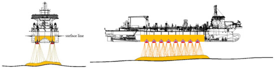
Figure 1. A schematic of the TSHD direct side-casting workflow.

During placement, the TSHD sails at a constant speed along grid lines. The precise control of the bottom door opening, coordinated with the pressure and discharge of the flushing/jetting system, promotes the orderly settling of the sand under gravity and ambient flow. Acceptable sand forms a jet-like fall as it passes through the doors; particle settling velocity in the water column is set by particle size and density, together with the surrounding flow field. The appropriate coordination of door opening and sailing speed regulates the areal spread and mound thickness, reducing the formation of local over-thick or weak zones. Throughout backfilling, the momentum coupling between the sand jet and the water column drives the preferential deposition of coarser fractions and densification of the basal layer, while finer particles disperse and settle with the flow. The resulting stratified accumulation enhances the overall quality of the backfill.

To ensure that the backfill thickness and surface planarity meet technical specifications, the workflow emphasizes end-to-end metrological feedback and closed-loop parameter control. Prior to placement, high-precision bathymetric surveys are conducted in the backfilling area and, in conjunction with the TSHD draft and local seafloor morphology, are used to design the casting grid and sailing routes, with rational spacing and coverage for each grid line. During operations, real-time measurements and equipment telemetry inform the dynamic adjustments of vessel speed, bottom door opening, and flushing discharge to finely control the thickness of each deposited layer. Upon completion of a pass, a timely bathymetric resurvey is performed to compare target thickness with as-built outcomes; spatial deviations are analyzed to optimize parameters for the next casting cycle, progressively achieving uniformity and continuity across the entire area. Grounded in the dual mechanisms of sediment dynamics and engineering control, the method stresses the coupled tuning between operational parameters and the hydrodynamic environment, ensuring uniform stratified accumulation and a dense basal structure, thereby reducing subgrade disturbance and subsequent settlement risk and forming a scientific, systematic, and dynamically optimized closed-loop regime for backfilling construction.

In backfilling operations, the main aim of layered control is to partition the total design thickness into a set of single layers and to impose strict control on the thickness of each layer. This approach reduces interlayer mixing and structural disturbance, improves subgrade uniformity and overall stability, and facilitates staged quality inspection. Specifically, the layer thickness should be optimized with respect to the properties of the basal mud layer, construction efficiency, and the technical specifications for backfilling. For example, when the design requires a total backfill thickness of 2 m, the operation can be executed in two layers, with each layer controlled within 0.5–1.0 m, and with the maximum single-layer thickness not exceeding 1 m, thereby balancing process efficiency and placement quality. Layered side-casting enables the sand to undergo uniform settlement and densification during progressive accumulation, markedly reducing the risk of subsequent differential settlement and subgrade instability.

To improve spatial coverage efficiency and thickness uniformity during the TSHD backfilling, the construction area is partitioned into parallel strips. Using the principal longitudinal axis of the site as a reference, strips are aligned parallel to this axis (Figure 2). The width of each strip depends on the effective sand coverage width of the TSHD (w_s) and the required overlap width between adjacent strips (w_c) to avoid edge underfill and weak zones. The actual strip spacing is as follows:

$$w_a=w_s-{\displaystyle \frac{w_c}{2}}$$

(1)

where w_a denotes the executed strip width (m); w_s denotes the effective side-casting coverage width (m); w_c denotes the overlap width between adjacent strips (m).

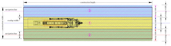
Figure 2. The grid layout for TSHD side-casting tracks (numbers 1–3 denote three parallel construction strips into which the working area is divided in space).

The overlap width is set by the edge-zone underfill: the mean lateral extent of the edge region whose thickness is below the pass-average thickness is considered and used as w_c.

The planned grid area is determined from the reported hopper volume and the target single-layer thickness. It is calculated using the following formula:

$$S_a={\displaystyle \frac{V_a}{h_a}}$$

(2)

where S_a denotes the planned spreading area derived from backfill volume (m²); V_a denotes the hopper volume reported by the TSHD (m³); h_a denotes the required single-layer backfill thickness (m).

This relation enables the back-calculation of the spatial extent required for each backfilling cycle and, together with the pre-established survey grid, guides the practical execution of side-casting tracks. After each pass, high-precision bathymetric surveys are conducted to verify and supplement the as-built spreading area and to compare it with the planned area, ensuring consistency between actual quantities and the schedule and enabling traceable, controllable project management.

2.2. CFD–DEM Modeling Framework for Layered Side-Casting Backfilling

In layered side-casting backfilling, the sand–water mixture discharged through the TSHD bottom doors enters the water column and undergoes complex dispersion, settling, and accumulation under the combined effects of gravity, hydrodynamic drag, and initial momentum. A coupled CFD–DEM framework unifies fluid and granular mechanics to simulate the complete particle kinematics in water.

During placement, sediment particles are released at the doors; the interaction between the carrier flow and the particulate phase jointly governs dispersion, settling, and mound formation. The coupled model resolves particle behavior under varying operating conditions—such as sailing speed and door opening—and quantifies their influence on plume spread. Specifically, the CFD component supplies the velocity and pressure fields, which drive DEM updates of particle positions and velocities; in turn, DEM-reported particle motion feeds back to the flow, altering local velocity and pressure distributions. This two-way coupling more accurately reproduces in situ dispersion–deposition processes of sediment particles, thereby providing a theoretical basis for predicting layer thickness and uniformity and for optimizing operational parameters during construction.

Assuming homogeneous, spherical sediment particles and a quiescent or uniform ambient flow, while neglecting turbulence and inter-particle collisions, the single-particle with particle-cloud approximation applies. For fine particles with d_p < 1 mm, the settling velocity is approximated using Stokes’ law:

$$v_{settle}={\displaystyle \frac{g({\rho }_p-{\rho }_w)d_p^2}{18{\mu }_w}}$$

(3)

where g represents the gravitational acceleration, ${\rho }_{\mathrm{p}}$ represents the particle density, ${\rho }_w$ represents the water density, d_p represents the particle diameter, and ${\mu }_w$ represents the dynamic viscosity of water.

For the representative TSHD sediment, consider $d_p=0.2$ mm, ${\rho }_p=2.65$ g/cm, and ambient-temperature water with $\mu =1.0\times {10}^{-3}$ Pa·s.

$$v_{settle}\approx 0.034\mathrm{m}/\mathrm{s}$$

(4)

If the water depth is 7.5 m (within the practical operating range), the following is established:

$$t_{settle}={\displaystyle \frac{h_w}{v_{settle}}}={\displaystyle \frac{7.5}{0.034}}\approx 220\mathrm{s}\approx 3.7\mathrm{m}\mathrm{i}\mathrm{n}$$

(5)

Sediment is discharged through the hull bottom doors with a finite initial horizontal velocity, governed by the door opening and flushing jets; the horizontal dispersion distance can be expressed as follows:

$$L=v_{0x}\cdot t_{settle}+0.5a_x{t}_{settle}^2$$

(6)

where $v_{0x}$ denotes the initial horizontal particle velocity (approximately the ship speed or the horizontal component at the door exit), $a_x$ denotes the horizontal acceleration under ambient flow, and $t_{settle}={\displaystyle \frac{h_w}{v_{settle}}}$ denotes the time required for particles to reach the bed.

Assuming dense-cloud settling, the backfill thickness per unit width is calculated as follows:

$$h_{fill}(x)={\displaystyle \frac{Q_s}{L\cdot v_s\cdot \Delta t\cdot {\rho }_{bulk}}}$$

(7)

where $Q_s$ represents the sand discharge rate (per unit time), $L$ represents the effective dispersion width, $v_s$ represents the vessel casting speed, $\Delta t$ represents the duration of a single pass, and ${\rho }_{bulk}$ represents the bulk density of the deposited sediment.

From the standpoint of physical media, the carrier phase is seawater, which is treated as an incompressible Newtonian fluid with density, ${\rho }_w\approx 1025 {\mathrm{kg}/\mathrm{m}}^3$, and dynamic viscosity, ${\mu }_w\approx 1.0\times {10}^{-3} \mathrm{Pa}·\mathrm{s}$. Over the relatively short simulation and construction times considered in this study, temperature and salinity are assumed constant, and large-scale thermohaline stratification is neglected; the water column is therefore represented by a single, homogeneous liquid phase whose motion is governed by the Navier–Stokes equations with gravity and, where relevant, free-surface effects.

The granular phase consists of non-cohesive, quartz-like sand representatives of TSHD backfilling projects. For the purposes of both the analytical estimates in this section and the subsequent CFD–DEM simulations, particles are modeled as homogeneous, rigid spheres with a single characteristic diameter, $d_p=2 \mathrm{mm}$, and density, ${\rho }_s\approx 2650 {\mathrm{kg}/\mathrm{m}}^3$. Cohesive fines, flocculation, and grain-size segregation are not explicitly resolved; instead, the focus is on the dominant behavior of the medium-to-coarse fraction that controls layer thickness and mound geometry. In the DEM submodel, each particle obeys Newton’s second law, with translational and rotational motion driven by the sum of contact forces and hydrodynamic forces. Normal and tangential contact forces are described by a soft-sphere spring–dashpot law combined with a Coulomb friction criterion. The fluid–particle interaction is represented by drag and buoyancy forces acting on each particle, with drag computed from standard correlations for spherical particles in water and projected along the relative slip velocity between the local fluid and the particle. Additional forces such as lift and virtual mass, as well as micro-scale lubrication forces, are neglected, which is acceptable given the relatively large particle size and the drag-dominated settling regime identified in the scaling analysis.

Within this simplified coupled description, the liquid phase captures the bulk hydrodynamic environment in which the granular phase moves and settles, while the granular phase provides a resolved representation of particle trajectories, collisions, and accumulation. Processes that are not included—such as the cohesive behavior of clay-rich suspensions, detailed rheology of highly concentrated mud layers, or long-term morphodynamic feedback between the evolving bed and the flow—may influence fine-scale structures in specific settings, but they do not alter the primary mechanisms or parameter sensitivities (bottom door opening, sailing speed) that this study aims to quantify on the engineering scale.

3. Numerical Simulation Study

3.1. Geometry Modeling and Scale Similarity Criteria

In this numerical simulation, the geometry model is primarily used to simulate the spatial environment of the trailing suction hopper dredger (TSHD) and its surrounding water domain. Using accurate geometric modeling, the interactions between the hull, bottom door, and flow can be reproduced, allowing for the prediction of sediment particle diffusion, settling, and accumulation behavior. The design of the geometry model considers not only the dimensions and shape of the vessel but also factors such as water depth, the topography of the construction area, and the vessel’s sailing path.

Given that both Computational Fluid Dynamics (CFD) and Discrete Element Method (DEM) models require extensive calculations and data processing, and considering the complexity of the actual TSHD and construction environment—such as turbulent water flow characteristics, vessel dynamic stability, and the heterogeneous distribution of sediment particles—the use of a numerically downscaled geometry is necessary to keep the computational load within a feasible range. In this study, the hull, hopper, and water depth are downscaled by a factor of 100 (a prototype water depth of 15 m represented by 0.15 m in the computational model; see Table 1), while the fluid and sediment material properties are kept equal to their prototype values. To maintain the correct balance between inertia and gravity for the free-surface jet and plume, the vessel speed is scaled by a factor of 10, such that the Froude number, $Fr=U/\sqrt{gL}$, is preserved between prototype and model. Taking the ship length as the characteristic length ($L_{\mathrm{p}}=72$ m) and a representative prototype speed ($U_{\mathrm{p}}=0.45 \mathrm{kn}$), the corresponding model values are $L_{\mathrm{m}}=0.72\hspace{0.25em}\mathrm{m}$ and $U_{\mathrm{m}}=0.045 \mathrm{kn}$, and the Froude numbers are equal ($F{r}_{\mathrm{p}}=F{r}_{\mathrm{m}}\approx 8.7\times {10}^{-3}$). Under these conditions, the Reynolds numbers are $R{e}_{\mathrm{p}}\approx 1.7\times {10}^7$ for the prototype and $R{e}_{\mathrm{m}}\approx 1.7\times {10}^4$ for the model (using $\nu =1.0\times {10}^{-6}{\mathrm{m}}^2/\mathrm{s}$), indicating fully turbulent flow in both cases; the remaining Reynolds number discrepancy mainly affects small-scale dissipation rather than the large-scale plume and deposition patterns.

Table 1. Geometry model parameters.

Parameter Name	Description	Unit	Actual Parameter Range	Scaled Parameter Range
Ship Length	Total length of the TSHD	m	72	0.72
Ship Width	Maximum width of the TSHD	m	26	0.26
Bottom Door Opening	Range of bottom door opening	/	[22%, 50%, 100%]	/
Ship Speed	Sailing speed of the vessel	kn	[0.2, 0.45, 0.70]	[0.02, 0.045, 0.07]
Water Depth	Water depth in the construction area	m	15	0.15
Grid Width	Width of construction grid	m	60	0.6
Grid Length	Length of construction grid	m	140	1.4
Particle Diameter	Sediment particle diameter	mm	2	2
Backfill Thickness	Maximum backfill thickness per layer	m	1	0.01
Ocean Current Speed	Ocean current speed	m/s	[0.1, 0.2, 0.3]	/

Because the sediment diameter is kept at the prototype value while the geometry is downscaled, the relative roughness ratios $d_p/H$ and $d_p/h_{\mathrm{layer}}$ are exaggerated in the numerical model compared to the field. This implies a larger apparent grain-scale roughness at the bed, which could in principle enhance local form drag within the thin interfacial zone where particles first come to rest. However, the final deposits in the simulations are typically tens of particle diameters thick, and the lateral spreading of the mound is governed primarily by the bulk momentum of the underflow and gravity-driven adjustment of the overall slope rather than by skin friction at the scale of individual grains. Any artificial increase in bed roughness introduced by the numerically downscaled prototype has, at most, a second-order influence on the lateral spreading under the present conditions. Nevertheless, this effect should be kept in mind when extrapolating the results to much finer sediments or exceptionally smooth seabeds.

For the particulate phase, the DEM uses prototype sediment properties (quartz-like sand with diameter, $d_{\mathrm{p}}=2 \mathrm{mm}$, and density, ${\rho }_{\mathrm{s}}\approx 2650 {\mathrm{kg}/\mathrm{m}}^3$), which are kept identical in the downscaled model. This choice intentionally departs from strict geometric similarity at the grain scale and follows the common “numerically downscaled prototype” approach, in which the real particle size is retained while the macroscopic geometry is reduced. The Stokes number, defined as $St={\tau }_{\mathrm{p}}U/L$ with ${\tau }_{\mathrm{p}}={\rho }_{\mathrm{s}}{d}_{\mathrm{p}}^2/\left(18\mu \right),$ which is the particle relaxation time, provides a measure of the relative importance of particle inertia and fluid time scales. Using a representative backfilling length scale ($L_{\mathrm{p}}=60 \mathrm{m}$) and prototype speed ($U_{\mathrm{p}}=0.4 \mathrm{kn}$), we obtain $S{t}_{\mathrm{p}}\approx 2\times {10}^{-3}$ for the prototype, whereas the downscaled model with $L_{\mathrm{m}}=0.6 \mathrm{m}$ and $U_{\mathrm{m}}=0.04 \mathrm{kn}$ yields $S{t}_{\mathrm{m}}\approx 2\times {10}^{-2}$. Although $S{t}_{\mathrm{m}}$ is about an order of magnitude larger than $S{t}_{\mathrm{p}}$, both values remain well below unity, indicating drag-dominated particle–fluid coupling and negligible ballistic lag in both cases. In other words, even with the geometry downscaled by 100:1 and the particle diameter unscaled, the settling and plume–bed interaction remain in the same dynamic regime (fully turbulent carrier flow with low-Stokes-number particles), and the dominant competition between advection, turbulent dispersion, and gravity is preserved.

Considering factors such as water depth and seafloor topography, the boundary conditions of the water region influence the flow distribution and the spread of sediment. The construction grid area is shown in Figure 3.

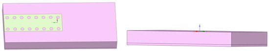
Figure 3. A schematic of the construction area model.

The model, which retains essential components such as the bottom door and reflects the vessel’s shape and dimensions, is shown in Figure 4.

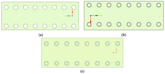
Figure 4. A schematic of the simplified vessel model. (a) 100% Opening; (b) 50% Opening; (c) 22% Opening.

It should be emphasized that the adopted 100:1 geometric downscaling is not a classical, fully similitude-complete physical model: the ratio of particle size to global water depth (e.g., $d_{\mathrm{p}}/H$) is indeed larger in the numerical model than in the prototype, and small-scale roughness effects associated with individual grains are exaggerated relative to the macroscopic geometry. Furthermore, the Stokes number in the downscaled model, although still well below unity, is higher than that in the prototype. As a result, the model is best interpreted as a numerically downscaled prototype that preserves the key dynamic regimes (Froude-scaled free-surface flow, fully turbulent Reynolds numbers, low-Stokes-number particle settling) rather than as an exact geometric replica at all scales. This implies that the quantitative thresholds reported in this study should be applied within the tested parameter ranges and interpreted together with the field validation, which demonstrates that the downscaled simulations reproduce the measured backfill thickness and footprint with acceptable accuracy for engineering design.

3.2. Numerical Boundary Conditions and Computational Setup

In the numerical model, water is treated as an incompressible Newtonian fluid with constant density, ${\rho }_w$, and dynamic viscosity, ${\mu }_w$, while the dispersed sediment is represented as a Newtonian granular phase with density ${\rho }_s$ and effective viscosity ${\mu }_s$. An Eulerian multiphase formulation is adopted, in which the volume fractions, ${\mathit{\alpha }}_q$, of the $q$-th phase (air, water, sediment) satisfy $\sum _q{\mathit{\alpha }}_q=1$. For each continuous phase, mass and momentum conservation are expressed as follows:

$${\displaystyle \frac{\partial }{\partial t}}\left({\mathit{\alpha }}_q{\rho }_q\right)+\nabla ·\left({\mathit{\alpha }}_q{\rho }_q{u}_q\right)=S_q^m$$

(8)

$${\displaystyle \frac{\partial }{\partial t}}\left({\mathit{\alpha }}_q{\rho }_q{u}_q\right)+\nabla ·\left({\mathit{\alpha }}_q{\rho }_q{u}_q\otimes u_q\right)=-{\mathit{\alpha }}_q\nabla p+\nabla ·\left({\mathit{\alpha }}_q{\tau }_q\right)+{\mathit{\alpha }}_q{\rho }_{q}g+M_q$$

(9)

where ${\alpha }_q$ is the volume fraction of phase $q$, ${\rho }_q$ is its density, $u_q$ is the phase velocity, $p$ is the common pressure field, ${\tau }_q$ is the viscous (including turbulent) stress tensor of phase $q$, $S_q^m$ is the inter-phase mass source term, and $M_q$ is the inter-phase momentum exchange term dominated by drag.

The latter is dominated by drag forces and is computed using a standard drag closure for dispersed solid particles in water. The air–water free surface is resolved using the Volume of Fluid (VOF) method, and the SST $\mathrm{k}$–$\omega$ turbulence model provides an eddy-viscosity closure for the water phase, as described earlier. At $\mathrm{t}=0$, the water column is at rest with a hydrostatic pressure distribution, and no sediment is present in the water column (${\alpha }_{\mathrm{s}}=0$) except within the bottom door region, where a prescribed mixture flux with given sediment volume fraction and velocity is imposed once the door opens. At the inflow boundaries, a specified velocity profile is applied, representing either quiescent ambient water or a uniform background current, while the corresponding sediment volume fraction is set to zero. The bottom and hull surfaces are treated as no-slip walls with a specified roughness height; the top outlet is modeled as an open-channel pressure boundary that allows free outflow of water and suspended sediment; and symmetry or far-field conditions are used at the lateral boundaries to minimize artificial reflection. This set of initial and boundary conditions defines the computational scheme for the transient Eulerian multiphase-VOF simulation of the side-casting jet, plume evolution, and near-field deposition.

The fluid and solid regions in the model are discretized using a nonuniform hexahedral mesh with local refinement in the bottom door jet region, the near-bed deposition zone, and along the free surface, while a gradually coarsened grid is adopted farther away from these dynamically active areas to reduce the overall cell count. This mesh layout ensures the adequate resolution of the jet, plume, and deposition processes within an acceptable computational cost. The resulting mesh distribution and locally refined regions are shown in Figure 5.

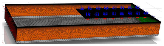
Figure 5. A schematic of mesh division.

Since the sediment plume dispersion process involves the interaction and collision of three phases, the model uses the Volume of Fluid (VOF) method, with the Eulerian phases representing air and water. Open-channel flow and implicit body forces are enabled, along with a surface tension model. The surface tension coefficient between the two phases is set to 0.0073 N/m, and the turbulence model used is SST k-omega.

Since the sediment plume dispersion process involves the interaction of multiphase flow and free-surface deformation, the Volume of Fluid (VOF) method is adopted to capture the air–water interface, and the Eulerian multiphase model is used to describe the water and sediment phases. The surface tension between air and water is set to 0.0073 N/m, and the turbulence model used is SST k-omega. The SST k-omega model is a two-equation eddy-viscosity closure that blends the advantages of the standard k-ε and k-ω formulations, improving predictions in the near-wall region and in free shear layers. However, as a Reynolds-averaged eddy-viscosity model based on the Boussinesq hypothesis, it does not explicitly resolve large coherent vortices, turbulence anisotropy, or small-scale shear-layer instabilities. In highly transient, particle-laden jets with stratification, such as the present bottom door discharge, this may lead to some over-smoothing of velocity and concentration gradients, particularly in zones of strong shear and density contrast. Consequently, local entrainment rates and peak concentrations in these regions are subject to additional uncertainty. Nevertheless, the SST k-omega-based RANS model reproduces the integral plume characteristics with acceptable accuracy for the engineering-scale analysis carried out in this study.

The inlet boundary is set to a constant flow rate or one that varies according to the tidal cycle, with specific parameters derived from on-site measured flow data. The pressure inlet is configured for open-channel flow, with secondary phase flow rates of 0.1, 0.2, and 0.3 m/s, and the inlet flow direction is set to both forward and lateral.

The outlet boundary is configured as an open-channel flow, based on the geometry model, to ensure the smooth discharge of sediment and water from the computational domain.

The bottom door of the TSHD, serving as the primary outlet for both sediment particles and flushing fluid, is set as a joint outflow boundary for particles and water. Parameters such as the bottom door opening (22%, 50%, 100%), discharge rate, and sediment mass flow rate (0.0233715 kg/s) are configured according to the actual construction process.

For particle–wall interactions (such as with the bed, hull, etc.), to reflect actual physical behaviors like deposition, rebounding, and friction, the elastic modulus, friction coefficient, and other dimensionless parameters are set as shown in Table 2.

Table 2. Dimensionless parameter settings.

Collision Interface	Collision Interface	Collision Interface
Static Friction	0.3	0.4
Dynamic Friction	0.3	0.35
Tangential Stiffness Ratio	1	1
Contact Stiffness Multiplier	1	1
Restitution Coefficient	0.3	0.3

In the DEM submodel, the sand backfill is represented by an assembly of non-cohesive, quartz-like spherical particles with a characteristic diameter, $d_p=2\hspace{0.25em}\mathrm{mm}$, and density, ${\rho }_s\approx 2650\hspace{0.25em}{\mathrm{kg}/\mathrm{m}}^3$. Each particle obeys Newton’s equations of translational and rotational motion:

$$m_p{\displaystyle \frac{d{u}_p}{dt}}=\sum F_{\mathrm{c}}+F_{\mathrm{d}}+F_{\mathrm{b}}+m_{p}g,I_p{\displaystyle \frac{d{\omega }_p}{dt}}=\sum T_{\mathrm{c}}$$

(10)

where $m_p$ and $I_p$ are the mass and moment of inertia of a particle, $u_p$ and ${\omega }_p$ are the translational and angular velocities, $F_{\mathrm{c}}$ and $T_{\mathrm{c}}$ are the resultant contact force and torque, $F_{\mathrm{d}}$ is the hydrodynamic drag force, $F_{\mathrm{b}}$ is the buoyancy force.

Particle–particle and particle–wall contacts are described by a soft-sphere linear spring–dashpot model in the normal and tangential directions. The normal contact force is given by the following equation:

$$F_n=k_n\hspace{0.17em}{\delta }_n+c_n\hspace{0.17em}{\dot{\delta }}_n$$

(11)

where $k_n$ represents the normal stiffness, $c_n$ represents the normal damping coefficient, and ${\delta }_n$ and ${\dot{\delta }}_n$ represent the normal overlap and its rate. The tangential contact force is expressed as follows:

$$F_t=-min\left({\mu }_f\hspace{0.17em}\left|F_n\right|,\hspace{0.33em}{k}_t\hspace{0.17em}{\delta }_t+c_t\hspace{0.17em}{\dot{\delta }}_t\right)$$

(12)

where $k_t$ and $c_t$ denote the tangential stiffness and damping, ${\delta }_t$ and ${\dot{\delta }}_t$ denote the tangential displacement and its rate, and ${\mu }_f$ denote the particle–particle (or particle–wall) friction coefficient. The corresponding contact torques are obtained from the moment of the tangential forces about the particle center. The stiffness, damping, restitution, and friction parameters used in the simulations are summarized in Table 2.

The sediment is introduced into the domain through the bottom door opening as a particle flux consistent with the prescribed mixture discharge rate. At each DEM time step, particles are generated within a source region just upstream of the door, with an initial velocity equal to the local carrier-fluid velocity plus a small random perturbation to avoid artificial ordering. The particle injection rate is adjusted so that the time-averaged solid mass flow matches the target volumetric concentration of the discharged mixture. The total number of tracked particles in each simulation is of the order of ${10}^5$, which provides sufficient resolution of the settling paths and deposited layer morphology while keeping the computational cost manageable.

The DEM integration time step $\Delta t_{\mathrm{DEM}}$ is chosen as a small fraction (typically 10–20%) of the Rayleigh time step associated with the stiffest contacts, ensuring the stable resolution of the contact dynamics. The CFD and DEM solvers are coupled in a staggered manner: several DEM sub-steps are performed within one CFD time step, $\Delta t_{\mathrm{CFD}}$, during which the fluid fields (pressure, velocity, and volume fraction) are held constant. At the end of each CFD time step, the local particle volume fraction and momentum exchange terms are re-assembled and fed back into the Eulerian multiphase equations through the drag source terms. In this way, the two-way coupling between the liquid and granular phases is captured at the time scales relevant to plume evolution and near-field deposition. Cohesive forces, particle breakage, and grain-shape irregularities are not included; the model thus focuses on the dominant dynamics of medium-to-coarse, non-cohesive sand that controls the engineering-scale backfill thickness and uniformity.

It should be noted that several simplifying assumptions are made in this formulation. The water is assumed to be isothermal, with constant density and viscosity; salinity, temperature stratification, and density variations induced by fine suspended sediment are neglected. The sediment is modeled as non-cohesive, spherical particles with a single representative diameter, so cohesive effects, flocculation, and grain-size segregation are not explicitly resolved. The seabed is represented as a fixed boundary during each simulation run, and long-term morphological feedback on the flow is not considered. Wave action, ship motion, and large-scale background turbulence are omitted, and the turbulence closure is based on a Reynolds-averaged eddy-viscosity model (SST $k$–$\omega$), which cannot resolve coherent vortices or small-scale intermittency in strongly sheared, stratified regions. These simplifications may lead to local errors in peak concentrations and fine-scale plume structure; however, the model reliably reproduces the integral behavior of the water–sediment system—namely, the settling paths, average backfill thickness, and spatial uniformity—which are the primary quantities of interest for the engineering-scale analysis in this study.

3.3. Mesh Independence Validation

Using nonuniform hexahedral meshes with local refinement around the bottom door jet region, the near-bed deposition zone, and the free surface, and gradually relaxed spacing in the far field, three structured grids were tested. For a representative case with an ambient current of 0.3 m/s, a vessel speed of 0.045 kn, and a 50% door opening, Figure 6 presents the temporal evolution of the domain-averaged backfill thickness for the three grids. All curves exhibit a consistent key response pattern, namely, a rapid rise to an early peak followed by decay towards a quasi-steady layer thickness, and the thickness remains strictly non-negative throughout. The auxiliary axis in Figure 6 shows the instantaneous absolute differences in average thickness between successive grids, indicating that the deviations of the coarser grids are modest: refinement from Grid1 to Grid2 already reduces the relative error to below 3%, while further refinement to Grid3 (5.3 × 10⁴) decreases the discrepancies to below 2%. Additional refinement yields only marginal improvement at the cost of a marked increase in computational time. Balancing accuracy and efficiency, Grid2 is therefore adopted as the engineering-optimal mesh for all subsequent simulations.

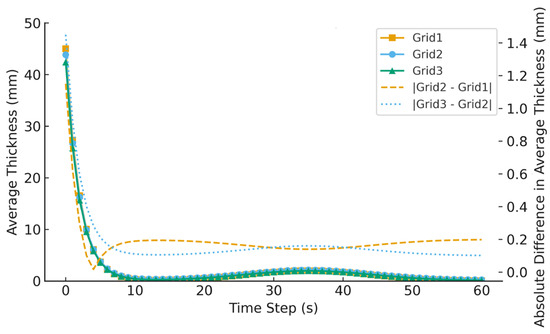
Figure 6. The average thickness for different grids.

3.4. Sediment Settling Path Analysis

Based on the orthogonal design, a systematic comparative analysis is conducted to evaluate the impact of bottom door opening (22%, 50%, 100%) and vessel speed (0.02, 0.045, 0.07 kn) on the diffusion and settling trajectories of sediment particles. For each set of conditions, scatter plots are used to illustrate the relationship between particle velocity and vertical settling depth. The primary focus is on comparing the distribution of the main settling cluster, velocity ranges, outlier distributions, and the uniformity of the deposited layers.

Under the 22% opening condition, the majority of particles settle near z = −0.14 m, with the horizontal velocity primarily distributed below 0.10 m/s and a relatively narrow main settling band. However, the low discharge flux and limited dispersion cause a strong contrast between the dense core and the very thin surrounding areas; at the footprint scale, this translates into pronounced thickness differences and a large uniformity index, i.e., poor areal uniformity despite the apparently compact settling band. As the vessel speed increases, some particles experience a slight increase in velocity, but the position of the main settling layer remains unchanged, and only a small number of outliers appear, as shown in Figure 7.

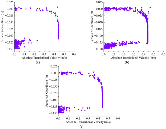
Figure 7. The sediment plume dispersion path at 22% opening. (a) 0.02 kn; (b) 0.045 kn; (c) 0.07 kn.

Under the 50% opening condition, the main settling band remains centered around z = −0.14 m, but the velocity distribution range expands to 0–0.25 m/s, and the width of the main settling group increases. The enhanced lateral dispersion allows the sediment to fill more of the effective footprint, reducing the contrast between the core and the margins; correspondingly, the final uniformity index drops to about 1.1, indicating a substantially more uniform thickness distribution than in the 22% opening case, even though the band edges exhibit slightly higher local shear, as shown in Figure 8.

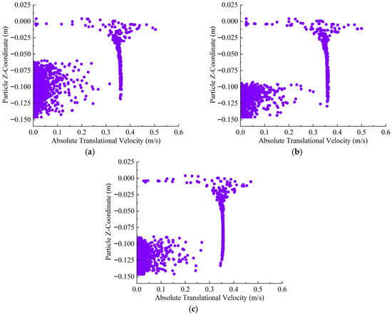
Figure 8. The sediment plume dispersion path at 50% opening. (a) 0.02 kn; (b) 0.045 kn; (c) 0.07 kn.

Under the 100% opening condition, the initial particle velocity increases significantly, with the velocity of the main settling group reaching up to 0.5 m/s and the settling band becoming much wider and more vertically dispersed. Some particles remain in the upper water layers and fail to settle promptly, and the particle density in the boundary regions decreases, leading to local deposition gaps. In terms of the uniformity index, this configuration yields a value of about 2.2—still far better than the 22% opening case but worse than the 50% opening—reflecting a trade-off between increased thickness and a partial loss of uniformity relative to the moderate opening, as shown in Figure 9.

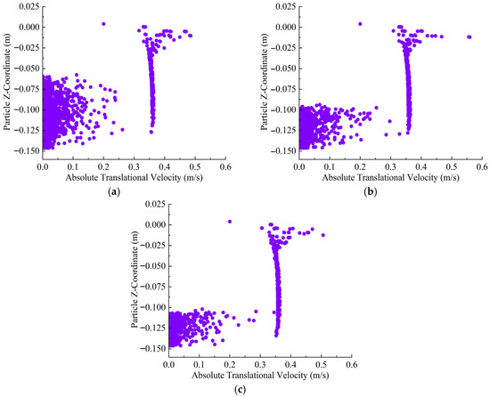
Figure 9. The sediment plume dispersion path at 100% opening. (a) 0.02 kn; (b) 0.045 kn; (c) 0.07 kn.

In summary, increasing the bottom door opening from 22% to 50% boosts the initial kinetic energy and dispersion in a way that both increases the final layer thickness and markedly improves areal uniformity (a lower uniformity index), whereas a further increase to 100% continues to thicken the layer but introduces more outliers and localized gaps, degrading uniformity relative to the moderate 50% opening while still remaining more uniform than the 22% opening case.

3.5. Sediment Deposition Morphology and Thickness Distribution Characteristics

To systematically analyze the effects of bottom door opening and vessel speed on backfill performance, three bottom door openings (22%, 50%, and 100%) and three vessel speeds (0.02, 0.045, and 0.07 kn in the model) were selected, with all other parameters kept constant. According to the adopted Froude-similar velocity scale (1:10), these model speeds correspond to prototype sailing speeds of approximately 0.2–0.7 kn. This range was determined from construction logs and typical practice for layered side-casting backfilling with TSHDs, where the vessel commonly operates at 0.3–0.6 kn to maintain a target layer thickness of about 0.4–1.0 m while avoiding excessive plume escape and edge irregularities. Prototype speeds lower than about 0.2 kn are seldom used in routine projects because they lead to very low construction efficiency, whereas speeds above 0.7–0.8 kn tend to produce underfilled, highly nonuniform layers. The three discrete levels (0.2, 0.45, and 0.7 kn on the prototype scale) were therefore chosen to span the practical operational window and to include slightly conservative lower and upper bounds for sensitivity analysis.

As shown in Figure 10, after the sediment is discharged from the bottom door, the particles primarily move along the longitudinal direction of the vessel, with the deposition band forming a “narrow elongated shape” and producing limited lateral diffusion. The thickness distribution exhibits a “bell-shaped” curve, with the maximum thickness at the center and a smooth transition at the edges, demonstrating high uniformity, which is suitable for precise thickness control. As vessel speed increases, the deposition band continues to extend longitudinally, and the particle diffusion distance at the leading edge increases, making the main deposition band longer, but with a reduction in thickness. Especially at high vessel speeds, some particles “escape” from the main band at the front edge, resulting in a sparse front edge of the deposition band. This indicates that high-speed flow combined with longitudinal flow is detrimental to uniform edge thickness control.

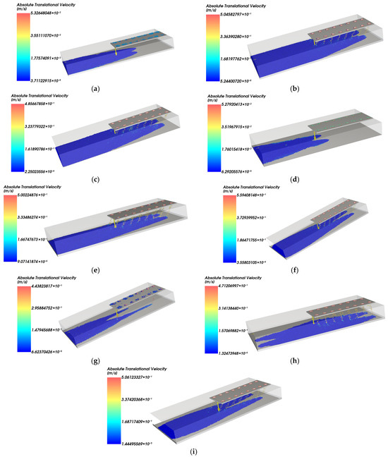
Figure 10. Near-field settling behavior under different sailing speeds and bottom-door openings (rows represent increasing sailing speed and columns represent increasing bottom-door opening). (a) 0.02 kn; 22% opening; (b) 0.02 kn; 50% opening; (c) 0.02 kn; 100% opening; (d) 0.045 kn; 22% opening; (e) 0.045 kn; 50% opening; (f) 0.045 kn; 100% opening; (g) 0.07 kn; 22% opening; (h) 0.07 kn; 50% opening; (i) 0.07 kn; 100% opening.

As the bottom door opening increases from 22% to 50% and 100%, the particle release rate rises, causing the longitudinal banded deposition area to widen in both the sailing and lateral directions, while diffusion still occurs predominantly along the vessel track. The stronger jet momentum and lateral dispersion at large openings spread the deposit out more: the local peak thickness along the plume axis for the 100% opening case becomes similar to, or slightly lower than, that at 50% opening because part of the flux is redistributed sideways. However, the much broader footprint and higher discharge flux lead to a clear increase in the footprint-averaged thickness. Coverage width, therefore, grows perceptibly with the opening, especially when increasing from 50% to 100%, and the thickness contrast between the core and the margins is partially reduced but accompanied by more pronounced local gaps at the band edges. Under maximum opening and high vessel speed, local deposition interruptions occur, with increased fluctuations in thickness at both the front and rear edges, leading to a decline in overall uniformity compared with the moderate opening case.

The small clusters of particles that remain beneath the vessel bottom and near the exhaust region in some panels of Figure 10 reflect grains that are trapped in a quasi-stagnant recirculation pocket formed between the downward jet and the hull. When the bottom door opening is small or moderate, and the vessel speed is relatively low, the jet tends to attach to the hull, generating a localized eddy with reduced shear and weak outward advection. In this case, a portion of the discharged particles loses momentum and accumulates in this sheltered zone, which appears as a cloud of low-velocity (cool-colored) grains beneath the door. As the door opening and/or vessel speed increase, the jet momentum and longitudinal advection become stronger, the recirculation pocket either shrinks or is swept downstream, and most particles are rapidly flushed into the main plume without long-term trapping.

In summary, the sediment deposition area generally takes on an elongated shape with a limited coverage width but relatively good thickness control. Increasing vessel speed widens the deposition band and tends to exacerbate edge fluctuations, reducing uniformity. For the door opening, moving from a small opening (22%) to a moderate opening (50%) not only slightly widens the band but also yields a marked increase in footprint-averaged thickness and the minimum uniformity index across the footprint, whereas further increasing the opening to a very large opening (100%) significantly widens the coverage and produces the thickest average layer, but reintroduces local gaps and edge irregularities. Consequently, a moderate bottom door opening combined with a moderate sailing speed emerges as the most robust configuration for balanced thickness control and uniformity.

4. Main Effect Analysis of Parameters

To quantitatively evaluate the spatial variation in the deposited thickness, a dimensionless uniformity index $I_u$ is introduced. In this study, $I_u$ is defined as the coefficient of variation in the backfill thickness field [22]:

$$I_u={\displaystyle \frac{{\sigma }_h}{\bar{h}}}$$

(13)

where $I_u$ denotes the uniformity index, ${\sigma }_h$ is the standard deviation of the backfill thickness within the analysis window, and $\bar{h}$ is the corresponding footprint-averaged thickness.

Then, a systematic analysis of the main effects of bottom door opening and vessel speed is performed, using two typical representative parameters: average thickness and uniformity. All data are derived from simulations conducted under the 0.02 kn operating condition. The x-axis represents the sedimentation time, while the y-axis corresponds to the average thickness and the uniformity index.

4.1. Impact of Bottom Door Opening on Average Thickness Evolution

The average thickness of the sediment layer is a key indicator for characterizing sediment settling and dispersion effects. Its variation not only reflects the rate and spatial distribution of sediment deposition during the initial discharge but also directly affects the uniformity and stability of the final backfill layer. Typical operating conditions with bottom door openings of 22%, 50%, and 100% and a vessel speed of 0.02 kn are selected to compare the evolution of average thickness under different parameters, as shown in Figure 11.

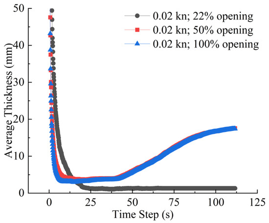
Figure 11. Time evolution of footprint-averaged backfill thickness under different bottom-door openings (22%, 50% and 100%) for the representative operating condition.

As shown in Figure 11, the average thickness follows a “high–low–slow increase” three-stage pattern across all bottom door openings. During the 0–10 s period, a large amount of sediment is released, causing the average thickness to rapidly reach its maximum value. For example, under 100% opening, the initial thickness can reach approximately 0.17 m, with 50% side opening at about 0.13 m and 22% opening at around 0.16 m. This indicates that the larger the opening, the stronger the instantaneous deposition capability and the higher the initial thickness.

During the 10–30-s period, the sediment is subjected to the spreading effects of water flow, and the average thickness rapidly decreases. For instance, with a 22% opening in the forward condition, the thickness drops from 0.16 m to approximately 0.01 m, a reduction of over 93%. In this phase, the sediment undergoes widespread diffusion and uniform distribution. After 30 s, the thickness gradually stabilizes. Data show significant differences in the final thickness under different conditions: approximately 0.004 m for the 22% opening, 0.021 m for the 100% opening, and 0.02 m for the 50% side opening.

The bottom door opening is the primary factor affecting the average thickness, as shown in Table 3. The time evolution of the footprint-averaged backfill thickness exhibits a two-stage behavior for the 50% and 100% opening cases. In the first stage (approximately 0–30 s), the average thickness rises rapidly as the dense underflow impinges on the bed and the bulk of the near-field discharge settles. In the second stage (after about 30 s), the growth rate slows down but remains positive: this slow increase is caused by particles that remain suspended in the recirculation region beneath the hull and in the dilute upper plume, which gradually lose momentum and settle back into the deposition footprint. The fraction of such slowly settling particles is larger at 50% and especially 100% opening because the jet is more energetic, penetrates higher into the water column, and spreads farther laterally, so that a non-negligible portion of the discharge is temporarily stored in the water column before returning to the bed. In contrast, at the 22% opening, the jet momentum and vertical reach are much smaller, the plume remains relatively compact, and most of the sediment settles within the first 20–30 s; consequently, the average thickness curve quickly approaches a plateau and shows almost no late-time increase.

Table 3. Initial and final average backfill thickness for different bottom-door openings.

Condition	Initial Thickness (m)	Final Thickness (m)
22% Opening	0.16	0.004
50% Opening	0.13	0.02
100% Opening	0.17	0.021

The higher initial peak of the 22% opening case (about 0.16 m) relative to the 50% opening case (about 0.13 m) is also consistent with this picture. With a small opening, the discharge flux is focused into a narrow band with limited lateral spread, and only a small fraction of the particles is carried into the upper water column; the early-stage deposit is therefore concentrated within a relatively small area and exhibits a pronounced local peak. For the 50% opening, the total solid flux is larger, but a greater portion of the discharge is advected and dispersed before settling, and the deposition footprint is already broader at early times. When averaged over the fixed evaluation window used to compute the footprint-averaged thickness, this broader but more weakly peaked deposit yields a lower initial average thickness, which is subsequently overtaken as the slowly settling particles return to the bed in the second stage.

At the 22% opening, the final footprint-averaged thickness is the lowest, and the deposit is both thin and highly sensitive to local variability, resulting in the highest uniformity index (poorest areal uniformity). At the 100% opening, the final footprint-averaged thickness increases from about 0.004 m (22%) to about 0.021 m, but localized mounds and edge fluctuations appear as the energetic jet spreads the deposit over a much broader area. The 50% opening provides an intermediate average thickness while achieving the lowest uniformity index, representing the best compromise between thickness control and lateral regularity. Noteworthily, the slight flattening of the local peak thickness along the plume axis for the 100% opening, described in Section 3.5, is a local effect caused by strong lateral redistribution and does not contradict the monotonic increase in footprint-averaged thickness reported by this study. Therefore, for large-scale, uniform thin-layer backfilling, a moderate opening is preferred, whereas very small openings should be used with caution, and very large openings are more suitable when maximizing local thickness and coverage is prioritized over strict uniformity.

4.2. Impact of Bottom Door Opening and Vessel Speed on Deposition Uniformity

In sediment backfilling operations, the uniformity of the deposition layer is a core indicator that directly reflects the construction quality and structural performance. A smaller uniformity index value indicates more consistent thickness across regions and a smoother overall distribution. A larger uniformity value, on the other hand, increases the likelihood of “deposition highlands” and “settling low points” within the construction area. Based on the conditions of 22%, 50%, and 100% bottom door openings and a vessel speed of 0.02 kn, a comprehensive analysis of the main effects on uniformity is conducted, as shown in Figure 12.

Figure 12. Uniformity evolution with dredging time.

Under the 22% opening condition, the sediment discharge rate is relatively low, with sediment concentrating near the outlet and rapidly settling. Initially, the uniformity increases briefly but then remains consistently above 20. The larger uniformity value indicates that the thickness distribution is highly uneven, with local thick deposits and thinner edges. Physically, at smaller openings, the sediment dynamics are insufficient for full dispersion, leading to significant thickness variations within the deposition range and imbalanced spatial distribution. It should be emphasized that this extremely large coefficient of variation does not reflect numerical instability, but is mainly a consequence of the very low footprint-averaged thickness. The deposit occupies only a narrow strip, such that most grid cells have thickness values close to zero, and even modest absolute deviations produce a very large ratio ${\sigma }_h/\bar{h}$.

Under the 50% opening and lateral current conditions, the uniformity shows a clear decrease, with its final value stabilizing around 1.1. This value is significantly lower than that for the 22% opening condition, indicating that under moderate opening conditions, the sediment can more fully diffuse over a greater distance and deposit across a wider area.

As shown in Table 4, for large openings, the final uniformity value is approximately 2.2, which is significantly better than that for the 22% opening condition, but slightly worse than that for the 50% lateral current condition. The high discharge rate at larger openings provides more kinetic energy to the sediment at the moment of discharge. Although the overall thickness increases, some particles can diffuse over long distances with the fluid, while others remain concentrated and settle locally. Therefore, the spatial distribution uniformity improves, but it does not reach the optimal level.

Table 4. Uniformity comparison.

Condition	Final Uniformity
22% Forward	20.7
50% Side	1.1
100% Forward	2.2

As shown in Figure 12 and Table 4, the backfill thickness and uniformity index do not vary as perfectly smooth functions of distance and time, but exhibit superimposed short-wave fluctuations. These oscillations are primarily physical in origin and arise from the inherently unsteady nature of the bottom door jet and sediment plume. The intermittent shedding of vortices and recirculation cells beneath the hull causes the episodic focusing or spreading of the particle-laden flow, so that local deposition alternates between slight overshoot and undershoot around the mean trend, especially near the plume axis and at the edges of the effective footprint. In addition, the granular phase is represented by a finite number of discrete DEM particles; when thickness statistics are computed over fixed spatial bins and finite time windows, the stochastic arrival and clustering of particles generate small-amplitude statistical noise that appears as short-scale ripples about the smooth envelope.

Importantly, these fluctuations remain bounded and do not grow in time, and their characteristic amplitude is small compared with the systematic differences between parameter combinations (bottom door opening and vessel speed). Mesh-independence checks and moderate changes in the temporal averaging interval lead to nearly identical envelopes of the thickness and uniformity curves, confirming that the main conclusions of this study are governed by the mean response and not by numerical instability. Therefore, the oscillations observed in Figure 12 should be interpreted as signatures of unsteady plume–bed interaction and particle discreteness superimposed on the underlying parameter-controlled trends, rather than as artifacts of the computational scheme.

In summary, relative to the small-opening case (22%), both moderate (50%) and large (100%) openings reduce the uniformity index and thereby improve areal thickness uniformity; however, the minimum uniformity index is achieved at the moderate opening, while the very large opening slightly sacrifices uniformity in exchange for additional thickness. Therefore, for optimal spatial thickness uniformity, a moderate opening of around 50% should be selected, and larger openings should be reserved for situations where additional thickness is required, and a modest loss of uniformity is acceptable.

5. Engineering Application Validation

Section 3 and Section 4 employ an orthogonal design with bottom door openings of 22%, 50%, and 100% and three vessel speeds to construct a parameter–response map over a broadened operating window around typical project conditions. This experimental design is intended to reveal systematic trends and identify robust operating ranges on the engineering scale. By contrast, the engineering validation in Section 5 relies on a second set of simulations configured with the actual construction parameters recorded for the Manila Pasay project, namely, bottom door openings of 10%, 15%, 20%, and 30% and vessel speeds of 0.3–0.5 kn (Table 5). These “field-case” simulations use the same CFD–DEM framework, mesh, and physical models as the orthogonal design, but their boundary and operating conditions are matched one-to-one to the site records and are used exclusively for comparison with the measured backfill thickness.

Table 5. Vessel speed and bottom door opening combination.

Serial No.	Vessel Speed (kn)	Bottom Door Opening (%)
1	0.3/0.4/0.5	10%/15%/20%/30%

5.1. Construction Conditions and Parameter Combination Design

To test the numerical simulation of layered side-casting backfilling by the trailing suction hopper dredger (TSHD) and validate the analytical results, the efficiency of the side-casting backfilling operation is verified. The simulation results are checked by conducting side-casting backfilling in the Pasay reclamation development project in Manila, Philippines. The construction equipment used is listed in Table 6.

Table 6. Construction equipment.

Serial No.	Equipment Type	Equipment Name	Technical Specifications	Quantity	Purpose
1	Trailing Suction Hopper Dredger	Junyang 1	Hopper capacity: 21,028 m3; cone-shaped bottom door radius: 2 m	1 vessel	Side-casting layered backfilling
2	Measurement Equipment	Survey Vessel	Equipped with multi-beam measurement devices	1 vessel	Pre- and post-side-casting measurements

In the TSHD layered side-casting backfilling process, the vessel speed and bottom door opening are key parameters that directly affect the effectiveness of the layered backfilling operation. Therefore, different combinations of vessel speed and bottom door opening are designed for comparison during construction, as shown in Table 5.

For each of the four representative parameter combinations adopted in the Pasay soft-foundation backfilling (door openings of 10%, 15%, 20%, and 30% combined with vessel speeds of 0.3–0.5 kn, see Table 5), a corresponding numerical “field-case” simulation is carried out using the same 1:100-scale CFD–DEM model described in Section 3.1, Section 3.2 and Section 3.3. The prototype vessel speeds and door openings extracted from the construction logs are converted to model-scale inflow velocities and opening widths according to the Froude-similar scaling used throughout this study, while the sediment properties, water depth, and ambient current are set to match the site conditions during the monitored runs. The mesh configuration, turbulence model, and fluid–particle interaction parameters are identical to those used in the orthogonal simulations, ensuring that any differences between the two simulation sets arise solely from the operating conditions rather than from changes in the numerical formulation.

5.2. Validation of the Correctness of the Numerical Model

Figure 13 shows the track chart of the side-casting backfilling tests. Using an RTK-GNSS high-precision positioning system, the TSHD side-casting numerical model was validated on the engineering scale; the deviations between the actual sailing tracks and the designed grid tracks are given in Table 7. Vessel position, heading, casting cadence, and the door open/close sequence were mapped to a moving source trajectory and time-dependent boundary conditions. The model inputs were synchronized with field settings—vessel speeds of 0.3/0.4/0.5 kn, door openings of 10/15/20/30%, wind speed, current speed, and high-pressure flushing—so that the external forcing and source strength matched the field conditions.

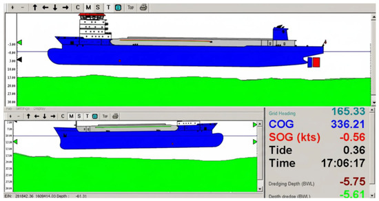
Figure 13. The track chart of TSHD side-casting backfilling tests.

Table 7. Side-casting backfilling construction efficiency.

Construction Voyage	Average Vessel Speed (kn)	Bottom Door Opening	Hopper Load (m3)	Wind Speed (m/s)	Flow Speed (m/s)	High-Pressure Flushing Pressure (bar)	Average Backfill Thickness (m)	Measured Backfill Volume (m3)	Sand Coverage Width (m)	Strip Construction Width (m)
1	0.3	10%	15,959	4	0.2	4.6	0.9	14,602	54	60
2		15%	15,849	4	0.2	4.6	1.0	14,422	55
3		20%	15,713	5	0.3	4.5	1.1	14,345	57
4		30%	15,516	4	0.2	4.6	1.2	13,964	58
5	0.4	10%	15,538	3	0.2	4.7	0.7	14,295	58
6		15%	15,927	4	0.2	4.6	0.9	14,732	59
7		20%	15,676	4	0.2	4.7	1.1	14,343	69
8		30%	15,685	5	0.3	4.7	1.1	14,273	60
9	0.5	10%	15,778	4	0.2	4.8	0.5	14,200	57
10		15%	15,673	4	0.2	4.7	0.6	14,105	58
11		20%	15,785	5	0.3	4.7	0.7	14,049	59
12		30%	16,048	6	0.3	4.6	0.8	14,266	63

Figure 14 compares the measured backfill thickness profiles along the survey transects with the corresponding “field-case” CFD–DEM simulations in which the bottom door opening and vessel speed are set to the same values as in the recorded construction runs. For all four parameter combinations, the discrepancy between the simulated and measured average backfill thickness along the track is minimal, with an absolute relative error not exceeding 4% and a mean absolute percentage error of about 2.3%. The coverage width and strip construction width match the field both in magnitude and trend: small openings with low-to-moderate speeds yield narrower coverage but better thickness control and smoother edges; as opening and speed increase, coverage widens slightly while edge fluctuations intensify and local dispersion increases.

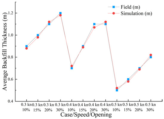
Figure 14. A comparison of average backfill thicknesses.

Discrepancies are concentrated at the leading edge and tail of strips for the large-opening plus high-speed cases. In conjunction with the wind–current data in Table 7, these zones are more sensitive to local resuspension, end-turn recirculation, and transient advection, producing minor deviations in the thin–thick transition bands. These are physically interpretable differences rather than systematic mismatches.

Examination of the temporal evolution of thickness shows three stages consistent with the field: rapid build-up with the discharge peak, subsequent decline and spreading under lateral entrainment and advective diffusion, and gradual stabilization. The model also reproduces systematic thickness drop-offs and enhanced local dispersion at track bends and strip ends, indicating that the numerical discretization of turbulent diffusion, interphase momentum exchange, and 3-D advection, as well as the time integration accuracy, satisfy engineering criteria and reasonably capture the deposition dynamics under side-casting operations. Overall, the spatiotemporal patterns and statistical levels of key responses are consistent with field trends; experimental (in situ) results and simulations agree well, demonstrating that the established CFD–DEM coupled method is rational and suitable for engineering applications.

5.3. Comparison of Backfilling Effects and Uniformity Evaluation

As shown in Table 7, the field backfilling tests on soft soil foundations mainly adopt vessel speeds of 0.3–0.5 kn with bottom door openings of 20–30%, which lie within the 0.2–0.7 kn operational window defined for the numerical parameter matrix. This consistency indicates that the simulated parameter space is representative of actual TSHD backfilling practice and directly supports the engineering relevance of the recommended parameter ranges. The on-site construction results indicate that, under different vessel speeds and bottom door openings, the average effective backfill volume percentage is 92%, showing good results. The average backfill thickness ranges from 0.5 m to 1.2 m, and multiple combinations meet the construction requirements. Specifically, when the vessel speed is 0.3 kn, bottom door openings of 10% and 15%; when the vessel speed is 0.4 kn, bottom door openings of 10% and 15%; and when the vessel speed is 0.5 kn, bottom door openings of 20% and 30% can effectively meet the construction requirements.

The vessel speed and bottom door opening combinations that result in an average backfill thickness between 0.8 m and 1.0 m are as follows: a vessel speed of 0.3 kn with bottom door openings of 10% and 15%, a vessel speed of 0.4 kn with a 15% bottom door opening, and a vessel speed of 0.5 kn with a 30% bottom door opening.

Since multiple combinations of vessel speed and bottom door opening yield good construction results, it is difficult to determine the optimal construction parameters based solely on the average backfill thickness. A further analysis of the construction effects is required. Therefore, the construction results for the above four combinations are further surveyed, with 30 additional measurement points added to cover the construction area. Based on the average backfill thickness (u), the standard deviation (v) is calculated and compared. The standard deviation reflects the degree of data dispersion and, to some extent, indicates the uniformity of backfilling and variations in thickness.

The comparison of construction effects for different combinations is shown in Figure 15. Figure 15a displays the backfill thickness at 30 survey points along the construction strip for each parameter combination, whereas Figure 15b summarizes, for the same four combinations, the corresponding average backfill thickness and standard deviation. In terms of average backfill thickness, Combination 2 performs the best, with an average thickness of 1 m. However, its standard deviation is 0.2, indicating a high level of data dispersion, meaning the backfill uniformity is relatively poor, with many measurement points exceeding 1 m in thickness. The reason for this is that the vessel speed is not very high, and as the bottom door opening increases, the backfill thickness tends to exceed 1 m.

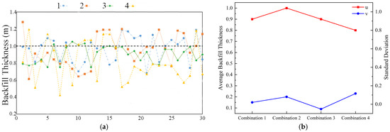
Figure 15. Comparison of construction effects for different combinations of vessel speed and bottom-door opening. (a) Backfill thickness at 30 survey points along the construction strip for the four parameter combinations. (b) Corresponding average backfill thickness and standard deviation for each combination.

As indicated by Figure 15b, Combinations 1 and 3 both have an average backfill thickness of 0.9 m. The standard deviations for these combinations are 0.09 and 0.15, respectively, with Combination 3 performing better due to its smaller data dispersion and fewer points with a backfill thickness greater than 1 m.

Combination 4 performs relatively poorly, with both a lower average backfill thickness and a higher data standard deviation compared to the other combinations. The reason for this is that the vessel speed is faster, and the bottom door opening is larger, leading to greater environmental influence, which causes uneven backfilling and poorer results compared to the other combinations.

Taken together, Figure 15a shows that Combination 3 maintains backfill thickness values clustered around the 1 m design line across most survey points, while Figure 15b confirms that it combines a near-target average thickness with one of the smallest standard deviations. Overall, Combination 3 delivers the best results, with an average backfill thickness close to the design target, a relatively small dispersion of measurement data, and better uniformity compared with the other combinations. Noteworthily, these comparative trends are obtained from an RANS simulation based on the SST k-omega turbulence model; in strongly sheared and stratified zones, small-scale intermittency and local peak concentrations may be smoothed; thus, the recommended parameter windows should be interpreted as engineering guidance rather than strict limits.

5.4. Discussion

The numerical and field results presented in Section 4 and Section 5 reveal a clear process-based structure in the response of the backfill system to changes in bottom door opening and vessel speed. Increasing the door opening primarily raises the initial discharge flux and jet momentum, which leads to a thicker deposited layer and a broader footprint, but also intensifies local shear and enhances small-scale variability in the plume–bed interaction. This explains why the average thickness increases almost monotonically with opening, whereas the uniformity index exhibits a non-monotonic response, with the strongest loss of uniformity occurring once the opening enters the high-momentum range. In contrast, sailing speed controls the balance between residence time and advective stretching of the dense underflow: low speeds favor locally concentrated deposition and thicker mounds, moderate speeds expand the lateral coverage without a severe penalty in uniformity, and excessively high speeds reduce residence time to the point where gaps and irregular edges emerge. The “medium–medium” combinations identified in Section 5.3 can therefore be interpreted as operating points where discharge momentum, residence time, and lateral spreading are co-tuned to maximize layer thickness within a given footprint while keeping the spatial variability of thickness at an acceptable level.

When compared with the existing studies on TSHD overflow plumes and near-field deposition, the study results are broadly consistent with previously reported trends but extend them in several important ways. Earlier laboratory flume experiments and depth-averaged plume models have shown that higher discharge momentum and vessel speed tend to enhance initial dilution and footprint width while reducing near-source thickness and promoting irregularity at the plume margins. Field monitoring campaigns around working TSHDs have similarly indicated that gentle sailing speeds and moderate discharge fluxes are conducive to more compact mounds and reduced far-field turbidity. The parameter windows identified in this study for layered side-casting backfilling (medium door opening, medium sailing speed) fall within the operational ranges reported in previous studies, but this study’s CFD–DEM framework resolves the three-dimensional settling of individual sand grains and quantifies the resulting layer thickness and uniformity index in a way that has not been reported previously. In this sense, the model acts as a process-based digital analog of the backfilling operation, translating controllable parameters into directly interpretable quality metrics (average thickness, coverage width, and uniformity index) that can be used for design and optimization.

At the same time, several limitations must be kept in mind when interpreting the findings. The sediment is represented as a monodisperse, non-cohesive granular phase, so cohesive fines, flocculation, and grain-size segregation are not explicitly modeled, and their contribution to long-range turbidity is only indirectly reflected in the results. The turbulence closure is based on a Reynolds-averaged eddy-viscosity model, which cannot resolve all coherent structures and intermittency in strongly sheared, stratified zones, and the bed response is treated quasi-statically within each simulation run without long-term morphodynamic feedback. In particular, the CFD–DEM framework focuses on the medium-to-coarse sand fraction that controls mound build-up and layer thickness, whereas non-settling wash load and fine suspended sediment, which are mainly responsible for far-field turbidity plumes in real dredging operations, are not resolved as a separate phase; as a result, the model reproduces the main mound geometry and near-field thickness patterns well but is likely to underestimate far-field suspended sediment concentrations and turbidity footprint, and should therefore not be used on its own for regulatory assessment of turbidity or ecological thresholds. These simplifications imply that the quantitative thresholds for “optimal” parameter ranges may shift in settings with markedly different sediment compositions, hydrodynamic forcing, or regulatory constraints. Nonetheless, the good agreement between the simulations and field measurements in Section 5.2 suggests that the dominant mechanisms and relative trends are robust, and the proposed parameter windows should be viewed as physically grounded guidance that can be further refined and localized using project-specific monitoring and calibration. Taken together, the orthogonal numerical results for 22–100% openings and the site-specific validation cases for 10–30% openings both point to an optimal regime at moderate bottom-door openings, so that a practical recommendation of approximately 15–50% can be regarded as robust: even though the parameter ranges in the two datasets do not perfectly overlap, the underlying physical trends in the trade-off between layer thickness and lateral spreading are fully consistent.

6. Conclusions

Based on the aforementioned systematic numerical simulations and experimental validations, this study comprehensively reveals the dominant role of two key process parameters—bottom door opening and vessel speed—on key quality indicators such as backfill thickness and uniformity. Combining parameter sensitivity results with practical engineering feasibility, this study proposes the recommended parameter ranges for layered side-casting backfilling and systematically demonstrates their significance in engineering applications.

(1)

Increasing the opening percentage from very small to moderate values (e.g., 22% to 50%) significantly enhances the initial kinetic energy and release flux of sediment particles, leading to thicker deposited layers, a broader spatial footprint, and a marked reduction in the uniformity index (i.e., improved areal uniformity). Further increasing the opening to very large values (100%) continues to increase thickness but causes a moderate rise in the uniformity index relative to the moderate case, indicating a trade-off between additional thickness and partially degraded uniformity. The approximately linear relationship observed between door opening and average thickness highlights its dominant role in vertical profile shaping, while the non-monotonic uniformity response underscores the existence of an optimum at moderate openings.

(2)

Low vessel speeds favor vertically concentrated deposition with a greater local thickness due to gravity-dominated settling and minimal lateral displacement. In contrast, moderate increases in sailing speed induce drag-induced sediment migration, effectively expanding the lateral coverage of the backfill layer. However, excessive speeds risk producing uneven thickness profiles and deposition gaps, particularly when combined with wide door openings.

(3)

The interaction between door opening and sailing speed reveals that uniformity cannot be optimized by tuning a single parameter. For instance, large openings require a compensatory reduction in speed to mitigate long-range particle migration and avoid nonuniform accumulation. Conversely, smaller openings permit higher speeds without significantly compromising uniformity. This interdependence underscores the necessity of joint parameter optimization in layered backfilling scenarios.

(4)

Field validation using the Junyang 1 TSHD in the Manila Pasay project confirms that a field-tested moderate bottom door opening of about 15%, selected in light of the simulated optimum occurring between 22% and 50% opening, paired with a moderate sailing speed of about 0.4 kn, provides an optimal trade-off between thickness control and uniformity, thereby verifying the applicability of the simulation-derived parameter windows under realistic construction constraints.

(5)

Field validation using the Junyang 1 TSHD in the Manila Pasay project confirms that a moderate bottom door opening (≈15%) paired with a moderate sailing speed (≈0.4 kn) provides an optimal trade-off between deposition thickness and spatial uniformity. This combination delivers stable, repeatable layer formation with minimal rework risk, offering practical guidance for quality control and operational planning in TSHD-based reclamation and subgrade backfilling projects.

(6)

From an environmental perspective, the recommended parameter window also contributes to reducing the far-field turbidity footprint. A moderate bottom door opening combined with a relatively low-to-medium vessel speed limits the initial momentum of the discharged jet and promotes earlier settling of coarse and medium-sized particles within the target footprint. As a result, the volume of fine sediment that can be advected into the far field is reduced, and the associated peak suspended sediment concentrations and plume extent are expected to decrease. Although a full far-field turbidity assessment is beyond the scope of this study, the identified parameter ranges are consistent with the concept of “green construction”, in which deposition quality and construction efficiency are improved while unnecessary dispersion of fines and ecological disturbance are restrained.

References

- Zhou, B.; Yu, M.; Guo, J. Hybrid optimization algorithm for estimating soil parameters of spoil hopper deposition model for trailing suction hopper dredgers. J. Intell. Fuzzy Syst. 2024, 46, 1813–1831. [Google Scholar] [CrossRef]
- Chen, L.; Zhang, X.; Pang, J.; Hong, G.; Chen, Z. Hydrodynamic Analysis of Trailing Suction Hopper Dredger with Opened Bottom Door. In Proceedings of the ISOPE International Ocean and Polar Engineering Conference, Rhodes, Greece, 16–21 June 2024; ISOPE: Geneva, Switzerland, 2024; p. ISOPE-I-24-570. [Google Scholar]
- Xia, Z.; Hong, Z.; Tang, R.; Song, S.; Li, C.; Ye, S. Research on Power Load Prediction and Dynamic Power Management of Trailing Suction Hopper Dredger. Symmetry 2025, 17, 1446. [Google Scholar] [CrossRef]
- de Wit, L.; van Rhee, C.; Talmon, A. Influence of important near field processes on the source term of suspended sediments from a dredging plume caused by a trailing suction hopper dredger: The effect of dredging speed, propeller, overflow location and pulsing. Environ. Fluid Mech. 2015, 15, 41–66. [Google Scholar] [CrossRef]
- Shao, M.; Wang, J.; Ding, X. Research on overflow diffusion characteristics of dredger. J. Phys. Conf. Ser. 2020, 1600, 012003. [Google Scholar] [CrossRef]
- Su, Z.; Zhang, X.; Yao, Y.; Zhu, D.; Fu, J. Mathematic modeling and CFD simulation of the sedimentation process in a TSHD. Mar. Georesour. Geotechnol. 2023, 41, 461–475. [Google Scholar] [CrossRef]
- Chen, Q.-Y.; He, Y.-P.; Xiong, T.; Li, M.-Z.; Liu, W.-H. Study on the dynamic characteristics of the overflow advection and diffusion of trailing suction hopper dredgers based on CFD. Ocean Eng. 2022, 252, 252111263. [Google Scholar] [CrossRef]
- de Wit, L.; Mosca, C.A.; Buschman, F.A.; Jaksic, L.; van der Deijl, E.; van der Biezen, T. Accurate Determination of Far-Field Source Terms of Barge Overflow Dredge Plumes Based on Near-Field Monitoring and Modeling. J. Waterw. Port Coast. Ocean Eng. 2025, 151, 04024026. [Google Scholar] [CrossRef]
- Mills, D. Predicting and measuring the characteristics of sediments generated by dredging. In Synthesis Report of Theme; Western Australian Marine Science Institution: Perth, Australia, 2019. [Google Scholar]
- Willemsen, M.P.J. An Analysis of Trailing Suction Hopper Dredger Dredge Plume Development and the Use of Suspended Sediment Source Terms; TU Delft: Delft, The Netherlands, 2022. [Google Scholar]
- van Rijn, L.C. One-Dimensional Plume Dispersion Modeling in Marine Conditions (SEDPLUME1D-Model). J. Mar. Sci. Eng. 2025, 13, 1186. [Google Scholar] [CrossRef]
- Miedema, S.A. An analytical approach to the sedimentation process in trailing suction hopper dredgers. Terra Aqua 2008, 112, 15–25. [Google Scholar]
- Hao, Y.; Tao, R.; Han, Z.; Yuan, C.; Zhang, L. Simulation and Prototype Measurements Analysis of Loading and Overflow Process of TSHD Hopper. In Proceedings of the GeoShanghai International Conference, Shanghai, China, 27–30 May 2018; Springer: Singapore, 2018; pp. 774–782. [Google Scholar] [CrossRef]
- de Wit, L.; Talmon, A.; van Rhee, C. 3D CFD simulations of trailing suction hopper dredger plume mixing: Comparison with field measurements. Mar. Pollut. Bull. 2014, 88, 34–46. [Google Scholar] [CrossRef] [PubMed]
- Smith, S.J.; Friedrichs, C.T. Size and settling velocities of cohesive flocs and suspended sediment aggregates in a trailing suction hopper dredge plume. Cont. Shelf Res. 2011, 31, S50–S63. [Google Scholar] [CrossRef]
- Su, Z.; Zhang, X.; Luan, R. CFD simulation and model predictive control of the pipeline transportation system in a trailing suction hopper dredger. J. Hydroinform. 2022, 24, 730–748. [Google Scholar] [CrossRef]
- Decrop, B.; Sas, M.; De Mulder, T.; Toorman, E. Large-eddy simulations of a sediment plume released by a dredger using overflow. J. Appl. Water Eng. Res. 2018, 6, 62–69. [Google Scholar] [CrossRef]
- Symonds, A.M.; Erftemeijer, P.L.; White, R.E.; Pastorelli, F. The influence of flocculation in turbid plumes from mechanical and hydraulic dredging. Cont. Shelf Res. 2024, 277, 105263. [Google Scholar] [CrossRef]
- Fonias, E.N.; van Eekelen, E.; Bosch, B.v.D. Fine Sediment Dispersion in the Addu-City Dredging and Reclamation Project. J. Mar. Sci. Eng. 2025, 13, 489. [Google Scholar] [CrossRef]
- Wolf, T.; Breugem, W.A.; Verheyen, B.; Decrop, B. Two-way-coupling near-field and far-field models for the simulation of plumes. In Proceedings of the XXIX TELEMAC Users Conference, Karlsruhe, Germany, 12–13 October 2023. [Google Scholar]
- Saffari, M.; Kianoush, P. Integrated petrophysical evaluation of Sarvak, Gadvan, and Fahliyan formations in the Zagros Area: Insights into reservoir characterization and hydrocarbon potential. J. Pet. Explor. Prod. Technol. 2025, 15, 54. [Google Scholar] [CrossRef]
- Pellegrini, C.; Sammartino, I.; Schieber, J.; Tesi, T.; de Mendoza, F.P.; Rossi, V.; Chiggiato, J.; Schroeder, K.; Gallerani, A.; Langone, L.; et al. On depositional processes governing along-strike facies variations of fine-grained deposits: Unlocking the Little Ice Age subaqueous clinothems on the Adriatic shelf. Sedimentology 2024, 71, 941–973. [Google Scholar] [CrossRef]
Disclaimer/Publisher’s Note: The statements, opinions and data contained in all publications are solely those of the individual author(s) and contributor(s) and not of MDPI and/or the editor(s). MDPI and/or the editor(s) disclaim responsibility for any injury to people or property resulting from any ideas, methods, instructions or products referred to in the content. |
© 2025 by the authors. Licensee MDPI, Basel, Switzerland. This article is an open access article distributed under the terms and conditions of the Creative Commons Attribution (CC BY) license (https://creativecommons.org/licenses/by/4.0/).