


Abstract
The Ordovician No. 6 fault zone reservoir in the Shunbei Oilfield exhibits ultra-deep-burial, high-pressure, and high-temperature conditions. Its pronounced tectonic control and significant heterogeneity render traditional in situ stress prediction methods—based on linear elasticity and anisotropy assumptions—inadequate for accurately characterizing the evolution and uncertainty of carbonate reservoir stiffness. Therefore, quantitatively predicting the development patterns and distribution characteristics of the Shunbei No. 6 structural fault zone is crucial for the exploration and development of Ordovician carbonate reservoirs in the Shunbei region. This study integrates wave impedance inversion with high-confining-pressure PFC particle flow biaxial test results to establish a constitutive calibration system consistent with seismic and experimental data. It introduces a nonlinear weakening function incorporating higher-order derivative constraints to fuse structural fracture and effective stress weakening effects, enabling dynamic correction of elastic parameters. This approach establishes a novel in situ stress prediction model. Simulation results indicate a predicted range for maximum horizontal principal stress between 201 and 261 MPa, with minimum horizontal principal stress ranging from 124 to 173 MPa. Predicted stress values for three key wells exhibit measurement errors within 6.92% compared to actual logging data, displaying a zoned spatial distribution consistent with regional tectonic stress evolution patterns. Simultaneously, sensitivity analysis reveals that the Young’s modulus fitting accuracy improved from 0.89 to 0.95, with a 43% reduction in mean square error, with the proportion of outliers reduced to below 1%. This significantly enhances response continuity and numerical stability in high-gradient disturbance zones and stiffness drop regions. The new model explicitly incorporates the nonlinear coupling between fracture geometry and pore pressure disturbance into the parameter field, eliminating systematic bias along fracture zones. Higher-order derivative constraints suppress numerical oscillations in high-gradient areas, stabilizing variance and preventing anomaly propagation. Residual distributions exhibit enhanced symmetry and reduced spatial autocorrelation, effectively suppressing numerical oscillations and divergence in complex fracture zones while significantly improving stress prediction accuracy for the study area. Overall, this research provides novel methodologies for predicting in situ stresses in ultra-deep carbonate reservoirs, offering engineering guidance and parameterization references for scheme deployment in complex fractured karst systems.
1. Introduction
In recent years, the deep and ultra-deep Ordovician carbonate reservoirs in the Shunbei area of the Tarim Basin have become key target zones for increasing oil and gas reserves and production. The reservoirs in this region are distinguished by their substantial burial depth, elevated temperature and pressure, compact rock properties, and well-developed fractures and karst cavities [1]. In such conditions, the precise characterization of subsurface stress variations is paramount for structural interpretation, evaluating wellbore stability, and designing fracturing programs. It also exerts a direct influence on reservoir enhancement efficiency and development deployment outcomes [2,3,4]. Within strike-slip fault zones, a variety of factors have been identified as contributing to variations in the magnitude and direction of the modern in situ stress field. These include differing tectonic segments (extensional, compressible, and translational), varying fracture strengths, distinct lithology, differing fracture orientations, and varying scale [5]. It is noteworthy that localized stress field anomalies have become a critical factor affecting oil and gas exploration and development. Consequently, traditional stress prediction methods are unable to satisfy the requirements of precision and stability. In the context of deep, complex structural reservoirs characterized by ultra-deep strike-slip faults, the spatial distribution of the stress field is notably intricate, exhibiting a high degree of heterogeneity [6]. Local stress anomalies have emerged as significant constraints on drilling safety and efficient development [7].
Byerlee proposed that sectional slip is governed by a critical friction criterion [8]. Morris and Olson further introduced a coupled normal stress-shear stress model to assess fracture slip potential [9]. Hickman’s work, integrating experimental data [9,10], demonstrated that faults in a critical slip state exhibit enhanced permeability [11]. However, due to high coring costs, experimental challenges, and technical barriers, in situ stress testing on ultra-deep cores remains difficult to implement. This phenomenon results in an absence of high-precision measured data that could provide a more detailed understanding of the stress distribution characteristics within fractures [12]. Consequently, this restricts the ability to describe local stress fields in greater detail. This approach also fails to consider the regulatory effect of fracture slip on permeability under high-stress conditions, thus failing to meet practical demands for identifying geological sweet spots and optimizing well locations in deep strike-slip faults controlling hydrocarbon reservoirs. It has been demonstrated that this situation serves to compound the already considerable paucity of research on the subject of local stress disturbance characteristics in strike-slip faults under ultra-deep, high-temperature, high-pressure, and highly heterogeneous conditions [13,14,15].
Zoback revealed that faults with an angle of approximately 30° between strike and maximum horizontal principal stress are more prone to shear slip [16]. As demonstrated by Agosta, Hennings and Becker, a significant coupling relationship has been confirmed between fracture volume fraction and pore fluid pressure through outcrop analysis [17,18,19], well productivity evaluation, and 3D modeling. However, numerical simulations of in situ stress fields primarily rely on finite element analysis [20]. In the construction of precise numerical models, initial and boundary conditions exert a substantial influence on the ensuing computational results. The failure to incorporate real fracture morphology, rock mass heterogeneity, and multi-phase tectonic superposition effects has limited in-depth exploration of in situ stress perturbation mechanisms [21]. Furthermore, the absence of accurate predictive models for quantitatively characterizing local stress anomalies in ultra-deep strike-slip fault zones prevents the early identification of high stress concentration zones and potential instability zones in engineering applications. This has the potential to engender considerable uncertainty with regard to drilling design and wellbore stability control [22].
In the field of fracture zone property evaluation, conventional methodologies predominantly concentrate on shallow fracture structures and filling characteristics, thereby proving ineffective in addressing the disturbance mechanisms and engineering response processes of localized in situ stress fields in ultra-deep strike-slip fracture zones [23]. The prevailing mainstream in situ stress modeling methods are predominantly founded on classical elastic mechanics frameworks. These include Kirsch’s analytical solution for elastic circular holes, the fracture pressure inversion model established by Hubert and Willis, and Zoback’s extended method for estimating in situ stress based on well logging and seismic coupling [24,25]. These methods typically assume the medium is isotropic, linearly elastic, and homogeneous, offering model simplicity and computational efficiency. Consequently, these technologies are extensively employed in shallow oil and gas blocks and regions characterized by uncomplicated tectonics. However, the Shunbei area is distinguished by the presence of a substantial strike-slip fault system comprising a variety of tectonic types. Reservoirs are buried at depths in excess of 7000 m, and drilling measurements indicate maximum horizontal principal stresses reaching 250 MPa in target layers, with minimum horizontal principal stresses still exceeding 140 MPa [26]. Under such high-stress conditions, distinct tectonic segments exhibit significant variations in fracture activity, pore pressure, and reservoir properties. The nonlinear coupling between the fracture system and pore fluids is markedly enhanced [27,28,29,30], leading to systematic biases in boundary responses and mechanical parameter assignments within traditional models. The spatial distribution of in situ stress often exhibits pronounced heterogeneity and local perturbations, with dramatic variations in the stiffness field. Conventional models have been found to be deficient in their capacity to adequately capture phenomena such as shear softening, local stress relief, and effective stress jump processes that are triggered by fracture activity [31,32,33,34,35,36].
The present paper achieves cross-scale unification from seismic properties to particle-level constitutive behavior by coupling macroscopic elastic parameters derived from three-dimensional wave impedance inversion with microscopic mechanical parameters extracted from high-confining-pressure PFC numerical experiments. Secondly, the paper develops a differentiable and physically constrained nonlinear weakening function using fracture volume fraction and pore pressure as core control variables to dynamically correct the elastic modulus field. This characterization accurately encapsulates the evolution of stiffness driven by coupled effects such as fracture slip, stress release, and fluid disturbance. Building upon this foundation, a higher-order derivative control mechanism is employed to constrain the model’s response surface boundaries, thereby suppressing nonphysical oscillations and numerical instability caused by abrupt stiffness changes. This enhancement is pivotal in ensuring the model’s stability and convergence, particularly in regions characterized by high stress gradients. The efficacy of the method is substantiated by a comprehensive verification process against measured data from key wells in the Shunbei area. This verification process attests to the model’s capacity to accurately delineate the spatial heterogeneity of the in situ stress field. The prediction results demonstrate a high degree of consistency with field measurements, thus outperforming existing traditional elastic mechanics models. This research provides a multi-scale coupling between microscopic rock mechanical behavior and macroscopic stress fields, and the proposed approach significantly improves the accuracy of in situ stress prediction in ultra-deep carbonate reservoirs. This integrated method provides a new pathway for quantifying stress heterogeneity and guiding wellbore stability design in structurally complex fault zones.
2. Geological and Structural Setting
The Shunbei Block is situated in the northern part of the Shuntu Gor Depression (Figure 1). This study area exhibits a distinctive hydrocarbon accumulation pattern, with tectonic features conducive to hydrocarbon trapping. Vertically fed source rocks, combined with faulting and karstification, have formed a unique hydrocarbon trap system. Abundant oil source rocks have facilitated long-term hydrocarbon migration and accumulation, ultimately forming a distinctive fracture-karst reservoir. Situated at the tilted terminus of the South Asian uplift, the area hosts a northeast-northwest trending strike-slip fault system. Strike-slip faulting represents the dominant tectonic deformation mechanism. As faults traverse multiple stratigraphic units, carbonate rocks within the fault zone undergo stress-induced metamorphism and fracturing, generating natural fractures that constitute fracture reservoirs. Concurrently, dissolution processes have formed cavernous reservoirs dominated by karst caves. Moreover, near these cavities, fracture-cavity reservoirs with well-developed natural fractures have been identified. Consequently, reservoir types can be broadly categorized into three: cavity reservoirs, fracture reservoirs, and fracture-cavity reservoirs.
Figure 1.
Regional Location Map of the Shunbei Study Area.
Extensive early research unequivocally established the indisputable correlation between observed hydrocarbon accumulations in the Shunbei area and the region’s extensive strike-slip fault activity. The primary strike-slip fault zones exhibit distinctive characteristics, including longitudinal bedding, planar segmentation, and multi-phase vertical superposition. Collectively, these features introduce significant uncertainties in hydrocarbon production and development. Figure 2 presents the Shunbei 6 Fault is situated within the saddle-shaped structural zone between the Awati and Mangger basins, extending over 120 km. Its principal strike is northeast, with horizontal offsets reaching 300–800 m and vertical displacements of 50 to 200 m. The primary manifestation of the studied phenomena is shear displacement, distributed between Faults 4 and 8, forming a complex geological structure interwoven with faults and folds [37,38,39]. The main study interval is the Ordovician Jianfang and Yingshan Formation carbonate reservoirs (T78 to T80) at burial depths of 7500 to 8500 m. This fault system vertically traverses Cambrian to Ordovician strata, exhibiting horizontal segmentation: the western segment features steeply dipping faults, the central segment forms thrust fault steps, while the eastern segment displays a broom-like branching structure. The interweaving of faults and folds results in pronounced lithological variations and strong spatial heterogeneity [40]. The stress field region of Fault Zone 6, the primary focus of this study, is situated in the central–western portion of the entire fault zone. Due to the scarcity of key well data, the accuracy of in situ stress field prediction is somewhat compromised, rendering its prediction significantly more challenging than for the adjacent Fault Zones 4, 5 and 8.
Figure 2.
Schematic diagram of the study area for Geo stress prediction in Fracture Zone No. 6.
3. Methodology
3.1. Seismic Faces-Controlled Elasticity Parameter Inversion and Reservoir Characterization in Ultra-Deep Carbonate Reservoirs
P-wave impedance characteristics serve as a key sensitive parameter for distinguishing between reservoir and non-reservoir formations. Their precise acquisition is crucial for characterizing fracture-cavity features within reservoir bodies [41]. This study employs deterministic inversion techniques under phase-constrained conditions to precisely obtain P-wave impedance values and further reveal fracture-cavity characteristics within the reservoir. Figure 3 presents the two-dimensional section of wave impedance inversion derived from the SHZ41X-SHB6-3H-SHB601X seismic profile, covering depths between 7200 and 9600 m. This reveals the spatial distribution characteristics of stratigraphic wave impedance within the study area. The upper-middle section exhibits green to yellow-green low-impedance zones, whilst the orange-red regions in the middle-lower section represent high-impedance zones, corresponding to dense sandstone or carbonate reservoirs. Four primary stratigraphic interfaces are identified within the profile, exhibiting an overall gentle southeastward (rightward) dip controlled by the regional tectonic stress field. Localized undulations and faulting within the strata indicate significant tectonic reworking of the stratigraphic structure. Within the ultra-deep interval between 7600 and 8200 m, lateral variations in wave impedance are markedly pronounced, with distinct inter-layer contrast. Overall trends show progressively increasing burial depth, accompanied by a stepwise increase in wave impedance values with depth.
Figure 3.
Cross-sectional view of the well-linked phased-inversion P-wave impedance data volume for Fault Zone 6 (four stratigraphic layers: T74 (dark blue at 7500 m), T76 (light green at 8200 m), T78 (red at 8600 m), and T80 (light blue at 9200 m)).
3.2. Analysis of Elasticity Parameter Profiles and Reservoir Brittleness–Ductility Discrimination
Rock elastic parameters are closely related to in situ stresses in geological formations and are essential elements for constructing in situ stress calculation models. Therefore, when conducting stress prediction, the influence of rock elastic mechanics parameters must be fully considered. Based on phase-controlled wave impedance inversion results and other logging and seismic data, this study obtained elastic parameters such as density, Poisson’s ratio, and Young’s modulus for the T74–T80 stratigraphic section. The inversion results of these parameters show significant differences in elastic properties between vertical and horizontal directions within the T74–T80 formation. Notably, the Poisson’s ratio exhibits a nonlinear growth trend with depth (Figure 4a). The T74 layer shows the most prominent Poisson’s ratio anomaly, presenting a band-like distribution of high values, indicating that tectonic fractures significantly weaken rock elastic properties. The T76 layer demonstrates relatively low Poisson’s ratios (0.23–0.25) with significantly reduced and uniformly distributed anomalies, reflecting weakened fracture activity. The T78 layer shows enhanced Poisson’s ratio anomalies, forming inclined band-like distributions from the middle to the left side of the profile, indicating intensified fracture activity. The T80 layer reaches maximum heterogeneity in Poisson’s ratio, with high-value zones appearing as block-like or patchy distributions (0.28–0.29), suggesting further complexification of fracture-pore structures. Overall, as burial depth increases, the controlling effect of fracture development on elastic parameters gradually intensifies, leading to increased interbed heterogeneity in reservoirs.
Figure 4.
Cross-sections of elastic parameters along Fault Zone 6 (T74–T80). (a) Poisson’s ratio profile illustrating brittle–ductile heterogeneity and fracture-controlled anomalies. (b) Young’s modulus profile quantifying stratigraphic stiffness differentiation and its relationship to fracture–cavity clusters and burial depth (four stratigraphic layers: T74 (dark blue at 7500 m), T76 (light green at 8200 m), T78 (red at 8600 m), and T80 (light blue at 9200 m)).
The Yang’s modulus profile further reveals the sequential variation characteristics of rock stiffness in the T74–T80 stratigraphic section (Figure 4b). The continuous low-value zones in the profile closely align with the fracture-erosion cavity development areas, indicating that fracture clusters significantly reduce rock mass stiffness, which gradually diminishes with burial depth. The deep high-value zones reflect the hardening effect of limestone caused by high confining pressure and late-stage cementation, intensifying with stratigraphic burial. Scattered low-value zones appear in the shallow western part of the profile, suggesting that early erosion fracture zones were not fully reinforced by subsequent cementation. Overall, Yang’s modulus increases gradually with burial depth, yet low-stiffness zones persist.
Based on the post-stack seismic data of the Shunbei Fault Zone 6, a deterministic seismic impedance inversion constrained by phase control was conducted along the SHZ41X–SHB6-3H–SHB601X profile. By integrating interpreted stratigraphic interfaces of the T74–T80 sequences with well-log data, a well-to-seismic calibration was performed to ensure consistency in both time–depth correlation and wavelet phase. Continuous P-wave impedance profiles of the target intervals were then extracted, and a rock-physics-based dynamic–static conversion was applied to derive the corresponding elastic parameter volumes, including density, Poisson’s ratio, Young’s modulus, and shear modulus. Subsequently, at the key stratigraphic boundaries (T74, T76, T78, and T80), the inverted seismic elastic parameters were calibrated against well-log measurements, followed by interval-based statistical analysis and weighted averaging to obtain the representative parameter ranges for each formation (Table 1). These elastic parameters quantitatively characterize the spatial heterogeneity and stiffness anisotropy of the macroscale fractured–karst system. They provide essential input for the development of a nonlinear stiffness-weakening model driven by fracture volume fraction and pore pressure, and also constitute a critical foundation for subsequent elastic tensor field construction, microscale mechanical response calibration, and dynamic optimization of the coupled modeling framework.
Table 1.
Phased wave impedance inversion elasticity parameterization.
3.3. PFC Particle Flow Experiments and Calibration of Mechanical Micro-Parameters
To effectively replicate the depositional environment of ultra-deep carbonate reservoirs and the in situ mechanical characteristics of reservoir rocks, whilst elucidating the control mechanisms of confining pressure on rock mechanical behavior, sensitivity testing under simulated real confining pressure conditions was conducted on cores from the T74 to T80 intervals (Lianglitai Formation to Yingshan Formation) using the PFC3D biaxial compression system [42]. Figure 5 demonstrates significant variations in rock failure mechanisms and crack evolution patterns under different confining pressure conditions. At low confining pressures, the stress–strain curve shows rapid post-peak decline, exhibiting typical tensile failure with numerous randomly distributed cracks. When confining pressure reaches 40–60 MPa, peak stress increases markedly, with primary cracks gradually transitioning to shear-dominated failure. Although crack quantity decreases, their connectivity improves. Under high confining pressure conditions, peak stress growth slows significantly, and crack formation lags behind peak stress occurrence, resulting in “delayed instability” characterized by single dominant cracks penetrating through the rock while maintaining high residual strength. Higher confining pressures lead to fewer but more concentrated cracks with directional energy release. This indicates that while high confining pressure suppresses early instability failure, it facilitates the formation of oriented crack channels.
Figure 5.
Schematic of Stress Extrusion Mechanism in Particle Flow.
During initial loading, all five confining pressure cases show a rapid overall increase in axial stress as strain accumulates, although the curvature and tangent stiffness of the very initial segment differ slightly among the 91–129 MPa confining pressure levels (Figure 6). Subsequently, as longitudinal load increased, peak strength progressively heightened, with the stress required to reach peak values correspondingly escalating. Upon stress peak attainment, specimens progressively entered the yield stage, exhibiting a stress decline trend. However, when confining pressure approached the rock yield/fracture threshold, microcracks rapidly initiated and propagated, causing a abrupt drop in elastic modulus. This resulted in nonlinear softening and localized instability phenomena within the stress–strain curve. Due to variations in mineral composition, uneven bond strength of pre-existing fractures, and anisotropic microstructural effects induced by bedding structures and tectonic stresses [43,44,45,46]. Fracture initiation and pore connectivity exhibit high heterogeneity and directional dependence. This consequently leads to differentiated responses to confining pressure. Integrating core test data (Table 2), results under simulated equivalent confining pressures reveal a nonlinear increase in rock fracture strength with rising confining pressure. Young’s modulus rose from 47.68 GPa to 82.49 GPa, while Poisson’s ratio decreased from 0.241 to 0.218. Notably, fracture density peaks at 91 MPa confining pressure, indicating that brittle tensile fracture dominates the rock failure mechanism during the low-to-medium confining pressure phase. Conversely, at ultra-high confining pressures, hydrostatic pressure significantly inhibits fracture propagation, driving the rock towards plastic deformation. This mechanical response is highly consistent with field observations of Ordovician ultra-deep reservoirs, indicating that this phenomenon is closely related to the high-stress environment at the actual burial depth of the fracture zone (exceeding 7500 m).
Figure 6.
Cracking states of simulated rock specimens under different confining pressure conditions: (a–e) simulate settings with confining pressures of 91–129 MPa. (a) Stress–Strain Response and Fracture Evolution under PFC2D Numerical Simulation 91 (MPa); (b) Stress–Strain Response and Fracture Evolution under PFC2D Numerical Simulation at 98 (MPa); (c) Stress–Strain Response and Fracture Evolution under PFC2D Numerical Simulation 105 (MPa); (d) Stress–Strain Response and Fracture Evolution under PFC2D Numerical Simulation 118 (MPa); (e) Stress–Strain Response and Crack Evolution under PFC2D Numerical Simulation at 129 (MPa). Solid red lines indicate stress (or load) distribution profiles along the scanning axis, reflecting mechanical responses at different sample locations; dashed blue lines and short horizontal lines correspond to porosity (or pore opening) variations in horizontal and vertical directions, with ranges of internal pseudo-color rectangular ROIs marked. The colored rectangular regions display pseudo-color distributions derived from phase separation of micro/nano CT (or SEM) images in that area based on grayscale thresholds. Each color represents distinct structures: matrix, mineral particles, connected pores, and microcracks. As confining pressure increases, the number of cracks decreases, but the scale of interconnected cracks forming larger fissures grows, with crack development shifting from the specimen edges toward the center.
Table 2.
Simulated Rock Mechanical Parameters of PFC Biaxial Tests in the North 6 Fault Zone under Different Surrounding Pressure Conditions.
The 91–129 MPa confining pressure data in Table 2 should be parameters from the specimen pretreatment stage. The experimental setup has been optimized based on the Ordovician pressure gradient to ensure consistency between confining pressure conditions and the geological background of the target formation.
3.4. Multiscale Nonlinear Constitutive Weakening Characterization and Response Features
The evolution of elastic modulus in fracture-dissolution-type carbonate reservoirs is simultaneously governed by Structural stress unloading induced by fractures, which directly weakens the rock skeleton’s load-bearing capacity; Effective stress reduction caused by pore pressure increase, which indirectly softens the rock mass by altering stress pathways and through synergistic amplification effects. This often triggers significant local stiffness declines at fracture intersections and anomalous overpressure zones, leading to stress field redistribution [47,48,49]. Fracture development primarily affects overall stiffness by reducing shear modulus and bulk modulus, while pore pressure alters rock deformation response along effective stress pathways. Traditional approaches based on linear elasticity or treating fractures and pore pressure separately struggle to accurately capture this synergistic evolution and its non-stationary characteristics over time and space. To address these issues, a multiscale constitutive weakening characterization analysis is developed, integrating structural fracture terms, effective stress weakening terms, and nonlinear coupling amplification terms. This framework describes the weakening effects on reservoir Young’s modulus and shear modulus under the synergistic action of fracture volume fraction and pore pressure. The nonlinear correction function after weakening is defined as:
where is the weakened generalized elastic modulus; is the initial weakened modulus;is the weighting coefficient controlling the influence intensity of each physical mechanism; is the pore pressure (MPa); is the exponential coupling modulation factor; is the fracture volume fraction (%).
Compared to traditional linear weighting models, it offers greater expressive flexibility, particularly in regions with intense fracture development and overlapping high-pressure zones [50,51]. It can precisely describe phenomena such as abrupt stiffness drops, strong stress perturbations, or localized stiffness recovery. To precisely quantify the influence of fracture volume fraction and pore pressure on the modulus weakening function, this study conducted derivative analysis on both parameters, revealing their effects on material stiffness weakening sensitivity and system curvature trends. First-order derivatives quantify the direct impact of each parameter on weakening rates. Due to the presence of power functions and parameter ratios in the model, increasing crack volume fraction exhibits a sensitivity amplification effect. Concurrently, dominant mechanisms vary significantly across different crack density ranges. Correspondingly, the first derivative of the pore pressure term quantitatively describes the mechanism by which pore pressure perturbations influence weakening rates, delineating “effective stress-dominated zones” and “pore pressure-sensitive zones.” First, partial derivatives of Young’s modulus with respect to are calculated to coordinate weakening effects, establishing the following general weakening model.
Based on Equation (1), taking first-order partial derivatives with respect to fracture volume fraction and pore pressure yields Equations (2) and (3). These equations quantify the direct contribution of each parameter to the Young’s modulus weakening rate, revealing the relative influence of different dominant factors across reservoir environments. Here, denotes the original (unweakened) Young’s modulus (GPa); represents the sensitivity derivative of Young’s modulus with respect to fracture density (Pa); and denotes the sensitivity derivative of Young’s modulus with respect to pore pressure (Pa).
By combining Equations (2) and (3), we construct the Jacobian vector to describe the sensitivity of Young’s modulus to the two variables:
Taking the coupling between Poisson’s ratio and P-wave impedance response as an example: since the inversion process typically yields impedance distributions while the objective is to infer the response patterns of Poisson’s ratio and Young’s modulus, the first derivative of impedance response with respect to Poisson’s ratio is expressed using the chain rule:
where is the rock porosity; is the Poisson’s ratio; is the P-wave impedance. Applying the same derivation to Young’s modulus yields:
Furthermore, second derivatives characterize the concavity/convexity and inflection points of response curves. The second derivatives of fracture volume fraction and pore pressure (Equations (7)–(9)) reveal the response stages of weakening: When the second derivative is positive, the system enters a “saturated” phase where marginal effects of elastic modulus weakening diminish, and the modulus curve approaches a plateau or gradual transition zone; When the second derivative is negative, the system enters an “unstable” phase. At this point, minor perturbations can trigger nonlinear abrupt drops or accelerated degradation, forming highly sensitive critical points or brittle zones. Notably, the proposed “saturation–instability” partition complements the earlier “effective stress-dominated zone–pore pressure-sensitive zone” classification derived from first-order derivatives. The former emphasizes the phased characteristics of weakening processes, while the latter highlights spatial variations in dominant mechanisms. Integrating both approaches yields a comprehensive physical partitioning of reservoir stiffness evolution.
whereis the second derivative of Young’s modulus with respect to fracture volume fraction (Pa); is the second derivative of Young’s modulus with respect to pore pressure (Pa); is the fracture weakening index; is the pore pressure weakening index.
Particularly in the coupled high-fracture-density–high-pore-pressure zone, the cross-second derivatives exhibit pronounced asymmetry and abrupt transitions, reflecting degenerative coupling behavior under the synergistic control of fractures and pore pressure. This characteristic is especially pronounced in fracture convergence zones, high-pressure anomaly zones, or brittle–ductile transition zones, holding significant importance for identifying sudden drops in reservoir stiffness and predicting brittle instability windows.
where represents the second-order partial derivatives of the fracture-pore pressure coupling derivative terms with respect to fracture volume fraction (Pa), pore pressure (MPa), and their interaction. This analysis reveals the curvature, inflection points, and phased characteristics of the weakening curve.
When the second derivative is positive, the system enters a “saturated-type” response phase. As fracture density or pore pressure increases, the marginal effect of modulus weakening gradually diminishes, and the stiffness degradation rate flattens. This manifests as a plateau or gradual transition zone during weakening, with the modulus curve tending toward a plateau or gradual segment. Conversely, when the second derivative is negative, the system enters an “unstable-type” response phase. At this stage, even minor perturbations in fracture degree or pore pressure can trigger nonlinear abrupt drops or accelerated degradation of elastic modulus. This locally abrupt behavior forms highly sensitive critical points or fragile zones in parameter space, representing the most unstable regions in reservoir stiffness evolution.
4. Establishment of an In Situ Stress Calculation Model
4.1. Grid Cell Partitioning in Fracture Zone Regions
To highlight stress characteristics in key blocks and minimize errors, the study area was gridded. The domain comprises 5324 cells and 2701 nodes (Figure 7). The red region represents the periphery of Fault Zone 6, gridded at 500 × 500 resolution with 565 nodes and 973 cells; The innermost gray-white area represents the core zone of Fault Zone 6, meshed at 200 × 200 resolution with 2155 nodes and 3507 cells; the green fault zone was meshed at 50 × 50 resolution with 828 nodes and 922 cells. The core zone of Fault Zone 6 accounts for approximately 80% of the total mesh.
Figure 7.
Grid Model of Fault Zone 6 in Shunbei.
4.2. Boundary Conditions for Fracture Zone Regions
Numerous trial calculations were performed during the study process. For the extension-fracturing phase Model 5: Northern region constrained in the y-direction, free in the x-direction; Western region: constrained in the x-direction, free in the y-direction; Eastern and southern regions subjected to tensile stress approximately 130° in the SE direction over time. Weitering of the represented in situ stress prediction calculations was compared with single-well stress field magnitudes until satisfactory results were achieved (Figure 8). The resulting stress field direction resembled the present tectonic stress field of the Shunbei No. 6 Fault Zone and aligned well with characteristics such as the distribution and magnitude of maximum principal stresses in single wells. Consequently, Model 5 was selected as the final computational boundary condition (Table 3).
Figure 8.
Boundary conditions applied to the Shunbei 6 Fault Zone structure ((a): no offset boundary strip, (b): offset boundary condition).
Table 3.
Selection of Boundary Conditions for Shunbei Computational Model.
4.3. Numerical Simulation of Structural Faults
The study focuses on the Lower Ordovician stratigraphic interval [47,52]. Due to computational limitations and the complexity of numerical calculations, the structural morphology is represented numerically based on the t74, t76, t78, and t80 configurations to depict the fault’s structural form. The main body of Fault Zone 6 exhibits a simple strike-slip structure. Its local structural features will be simplified, with adjustments made later based on simulation results. The fault system primarily controls the structural pattern of the target stratigraphic interval, comprising 11 faults in total (Figure 9). The entire geometric model incorporates the major fault characteristics within the study area, objectively and accurately reflecting the complex geological landscape resulting from multiple episodes of tectonic activity.
Figure 9.
Numerical Simulation of Fault Structural Morphology.
4.4. Mathematical Computational Model
The model incorporates a pore pressure prediction method based on porous medium elastic mechanics and generalized Hooke’s law. By linking the skeletal modulus with the pore fluid modulus, it establishes a physical coupling relationship between elastic parameters and pore pressure. Building upon existing computational models, this study introduces a superpressure theory prediction method based on the quantitative relationship between pore pressure and rock elastic parameters:
where is the dry rock skeletal bulk modulus; is the rock matrix bulk modulus; is the bulk modulus of the fluid phase in the rock; is the mean principal stress. By incorporating the elastic mechanics of porous media and linking the skeletal modulus with the pore fluid modulus, a physical coupling relationship between elastic parameters and pore pressure is established.
By linking the skeletal modulus and pore fluid modulus, a physical coupling relationship between elastic parameters and pore pressure is established, thereby interconnecting the in situ stress field and overpressure field to form a complete response pathway. Based on this, the formulas for the maximum principal stress () and minimum principal stress () are derived:
where EH* and Eh* denote the elastic modulus after nonlinear weakening. νv, νH, νh are the isotropic Poisson’s ratios; σH and σh are the maximum and minimum principal stresses, respectively; and a is the stress adjustment factor.
Building upon Equation (10), the calculation methods for the maximum and minimum horizontal principal stresses are derived in Equation (11). This equation organically integrates the crack volume fraction, pore pressure, and elastic modulus weakening effect, enabling dynamic prediction from parameter perturbations to principal stress evolution. It signifies the comprehensive coupling of micro-scale weakening mechanisms with macro-scale stress response.
5. Results and Discussion
5.1. Sensitivity Curves of Poisson’s Ratio–Longitudinal Wave Impedance in Carbonate Reservoirs and Identification of Sensitive Zones in Fault Zones
The P-wave impedance exhibits a monotonically increasing trend with rising Poisson’s ratio, demonstrating a region of significantly enhanced sensitivity when the Poisson’s ratio falls within the 0.23–0.28 range (Figure 10). Within this interval, sensitivity increases from approximately 1.0 to 2.8–3.0, indicating that even minor variations in Poisson’s ratio can trigger substantial impedance responses. Meanwhile, under conditions where Young’s modulus ranges from 30 to 80 GPa, the curves undergo overall shifts while maintaining consistent variation patterns. Higher Young’s modulus corresponds to greater absolute impedance values, with the sensitive region marginally shifting toward higher Poisson’s ratios. These findings demonstrate that the impedance’s sensitivity to Poisson’s ratio is quantifiable and not linearly constant. Particular attention should be paid to the moderate Poisson’s ratio range around 0.25, which proves most effective for improving identification accuracy. Additionally, dual effects of localized stress concentration and crack plasticity enhancement require close monitoring.
Figure 10.
Sensitivity response of Poisson’s ratio to P-wave impedance. (A local positive correlation between Poisson’s ratio and P-wave impedance is observed in the inversion results, which mainly reflects the coupled effect of density increase and stress compaction rather than a direct physical causation).
5.2. Two-Parameter Nonlinear Weakening Simulation and Stress Evolution Analysis
Figure 11 illustrates the spatial distribution of normalized stiffness fields under simulated dual-parameter control, aiming to identify the nonlinear coupling mechanism between rock mass stiffness fields and geostress distribution. The study reveals that stress field evolution is not merely a linear superposition of crack effects and pore pressure effects, but rather governed by nonlinear coupling coefficients. This demonstrates a progressive transition from near-linear states to complex nonlinear and multipolar configurations.
Figure 11.
Two-dimensional nonlinear weakening distribution simulation. (Normalized stiffness field responses under different combinations of fracture volume fraction and pore pressure (schematic, dimensionless), used solely for pattern recognition).
In the early stage of low coupling (with crack volume fraction around 15–20% and pore pressure at 70–90 MPa), crack effects and pore pressure effects remain largely independent, exhibiting approximately linear stress responses. The maximum principal stress and shear stress generally maintain high numerical values with relatively uniform spatial distribution. Stress-weakening zones display symmetrical and concentrated characteristics, primarily regulated by a single dominant factor. As the coupling coefficient increases, the synergistic effects between crack and pore pressure effects intensify, leading to significant amplification of stiffness reduction and stress concentration phenomena.
During the medium-high coupling phase (with crack volume fraction of 25–35% and pore pressure of 100–140 MPa), the stress-weakening zone no longer exhibits a simple strip-like distribution. Instead, it evolves into complex structures including local minima islands, nested sub-regions, and asymmetric weakening zones. The maximum principal stress and shear stress decrease rapidly, with abrupt stress gradient changes. This demonstrates the coupling mechanism where “crack propagation reduces local stiffness, which further weakens load-bearing capacity through pore pressure disturbance,” ultimately triggering higher-order nonlinear responses and potentially leading to local instability.
In the extreme coupling region (with a fracture volume fraction of approximately 40% and pore pressure of 150 MPa), the nonlinear coupling coefficient reaches its peak. At this stage, the maximum principal stress drops below 50 MPa, shear stress falls under 20 MPa, and stress contour lines exhibit dense, fragmented patterns. Stress-weakening zones form isolated islands, creating a characteristic “engineering shield zone” or physical limit domain, indicating the system has entered a high-risk instability state.
In contrast, within the optimal equilibrium region (with crack volume fraction of 28–33% and pore pressure of 110–130 MPa), the nonlinear coupling coefficient remains moderate, where crack effects and pore pressure effects cancel each other out. The stress field exhibits continuous smoothness, with the attenuation of principal stresses and shear stresses controlled within 20–35%. The response surface gradient is uniform, demonstrating an overall controllable and stable operational window.
The nonlinear coupling coefficient γ serves as a pivotal parameter bridging microcrack evolution and macroscopic stress response. When γ is low, the system exhibits relatively independent mechanisms. As γ increases, a pronounced crack-pore pressure coupling effect emerges, causing stress-weakening zones to migrate and rapidly expand toward the upper-left corner of the domain. This asymmetric stress field evolution significantly heightens instability risks.
5.3. Nonlinear Weakening and Stress Release Mechanism
Nonlinear weakening simulations demonstrate that coupling fracture volume fraction with pore pressure significantly alters stress distribution patterns in carbonate fracture-cavity reservoirs. Under different combinations of conditions, this coupling evolves from quasi-linear behavior to asymmetric weakening and even extreme instability. Through systematic analysis of stress distribution patterns under fracture-pore coupling, this study categorizes five model groups describing stress control mechanisms across diverse geological scenarios. This reveals a nonlinear evolutionary sequence of reservoir fracture zone mechanical behavior—transitioning from stable dominant control to multipolar anomalies and ultimately to dynamic equilibrium. Furthermore, it quantitatively elucidates the variability and complexity of reservoir mechanical behavior under different coupling intensities and spatial structural conditions.
The standard stress distribution pattern (Figure 12) is dominated by a dual-parameter coupling mechanism involving fracture volume and pore pressure. The dominant zone manifests as a continuous, macroscopically smooth high-response channel, representing the “continuum-dominated” mechanism where the fracture network and pore pressure field exhibit highly synergistic interaction. The stress field exhibits a uniform gradient along the fracture zone direction, with local high-order perturbations effectively constrained by the dominant zone. This reflects the self-organizing regulation and stable distribution characteristics of elastic parameter fields in ultra-deep formations under complex mechanical coupling effects.
Figure 12.
Standard stress distribution pattern under dual-parameter coupling mechanism of fracture volume and pore pressure.
Figure 13 illustrates that under a multi-polar segmented scenario, the continuity of the fracture zone’s dominant band is disrupted by weakened nonlinear high-order perturbations, resulting in a multi-centered, segmented pattern of high-response zones. The coupling between fracture volume and pore pressure intensifies local stress concentration trends, inducing a multi-polar stress field distribution and forming a “cooperative dominant” regulation pattern. Significant interaction exists between the dominant zone and anomalous response areas, with highly dispersed stress pathways. This demonstrates the profound restructuring capability of the ultra-deep Ordovician fault zone’s heterogeneous structure and high-order nonlinear parameters on the mechanical field distribution. This model effectively reveals the coupled evolutionary patterns of local stress anomalies and multipolar response mechanisms within the complex mechanical environment of the fault zone.
Figure 13.
Multi-pole segmented synergistic dominant type.
A scenario where the dominant control zone exhibits spatial misalignment and interlaced distribution due to high-order nonlinear perturbations (Figure 14). The non-uniform coupling between fracture volume distribution and pore pressure anomalies induces multiple wavy interlacing patterns in the principal stress channels. The dominant control zone’s influence undergoes periodic amplification and attenuation under localized perturbations. This “misaligned and interlaced dominant control” regulatory pattern highlights the dynamic shaping capacity of fracture transitions, branch development, and multiscale heterogeneity on the spatial structure of the in situ stress field.
Figure 14.
Displacement-interlaced coupled dominant-control type.
Under multi-field coupled optimization, this stress field pattern exhibits highly coordinated spatial distribution of the dominant control zone with effectively suppressed local anomalies (Figure 15). The dual-parameter coupling mechanism of fracture volume and pore pressure enhances the continuity and dominance of the dominant control zone, while peripheral anomalies exhibit reduced response amplitude and smoother stress gradients. This pattern demonstrates the ability to spatially standardize elastic parameter fields and actively shield higher-order anomalies.
Figure 15.
Highly Coordinated Disturbance-Suppressed Dominant Control Pattern.
Stress regulation mechanism under the combined influence of the dominant zone and local anomalies. The overall structure of the dominant zone persists, but the high-response zone locally narrows, branches, and exhibits dynamic fluctuations at the boundary with the anomaly zone (Figure 16). Building upon the spatial continuity of the dominant control zone, multiple-point interactions occur between local high-response zones and the dominant control channel, manifesting as spatial narrowing, branching, and dynamic fluctuations. Driven by the high-order nonlinear coupling effects between fracture volume and pore pressure, stress regulation evolves from single-dominant control to dominant-anomaly synergy, forming a multi-scale dynamic equilibrium field. Figure 12, Figure 13, Figure 14, Figure 15 and Figure 16 are conceptual mechanism diagrams, designed to illustrate the coupled evolution among fracture volume fraction, effective modulus, stress redistribution, and energy release, rather than numerical outputs.
Figure 16.
Dynamic Equilibrium Model of Dominant-Local Anomaly Interaction.
5.4. Effect of Elastic Parameter Correction and Sensitivity Response Evaluation
Due to the complex pore structure and anisotropy of carbonate rocks, elastic parameters (Young’s modulus, shear modulus, etc.) dynamically vary with pore pressure, fractures, and other factors. Particularly in reservoirs with high pore pressure or extensive fracturing, rock elastic behavior becomes significantly more complex. Therefore, to overcome fracture zone interference terms and achieve precise representation of spatial heterogeneity and nonlinear response in elastic modulus under fracture-pore pressure interaction while incorporating actual geological zoning characteristics of fracture zones, multiple control parameters are included in the dual-parameter multiplicative weakening model [48,49,50]. multiple parameter combinations are set for use in correction functions for both seismically inverted elastic modulus profiles and PFC experimental data. This enables focused simulation of elastic stress field responses tailored to varying geological zoning and fracture-pore pressure dynamics.
Under various combinations of fracture sensitivity coefficient () and pore pressure sensitivity coefficient () (Figure 17), the normalized stiffness field response and its influence on principal stress distribution and numerical stability were investigated. Research indicates that when parameters are set to higher values (= 1.0, = 1.0), excessive stiffness field decay causes extreme stress concentration in the principal stress distribution. This leads to abnormal fluctuations in the condition number of the Jacobian matrix during simulation, significantly reducing numerical convergence and increasing the likelihood of simulation divergence. Conversely, when parameters are set to lower values (e.g.,= 0.4,= 0.2), the stiffness field becomes excessively smooth. This significantly weakens stress jumps and boundary effects in fracture clusters, failing to accurately reflect the complexity and heterogeneity of the rock formation. Through systematic parameter sensitivity analysis, the optimal parameter combination is determined to be = 0.65 and = 0.32. Under this parameter combination, the model exhibits stable and continuous spatial stress gradients, balanced principal stress distribution, natural boundary transitions, and smooth variations in the Jacobi condition number, achieving optimal overall numerical stability. Specifically, fracture clusters accurately capture stress drops and concentration phenomena, while non-fractured zones maintain smooth inter layer transitions, reasonably reflecting the structural heterogeneity and non-uniform stress distribution characteristics of actual reservoirs.
Figure 17.
Simulated stiffness field responses under different parameter combinations.
The optimal parameter combination (= 0.65,= 0.32) was applied to the nonlinear elastic parameter model of the Shunbei 6 fault zone for coupled correction. Comparative analysis revealed that post-correction, all physical parameters exhibited more linear and monotonic response trends within the primary variable spaces of and (Figure 18), significantly enhancing the continuity and trend consistency of parameter distributions. The corrected model substantially reduced high-frequency noise and random outliers in the original scatter plot distribution, with parameter standard deviation and mean squared error decreasing by over 30% on average (Figure 19), indicating effective suppression of experimental errors and stress perturbations. Particularly within the extreme parameter ranges, the upper and lower bounds for Young’s modulus, shear modulus, Poisson’s ratio, and density all converge within physically reasonable limits. The proportion of extreme outliers drops below 1%, avoiding the unstable oscillations generated by traditional models in high-order nonlinear regions.
Figure 18.
Comparison of elastic parameter corrections: (a) Young’s modulus comparison, (b) shear modulus comparison, (c) Poisson’s ratio comparison, (d) density comparison.
Figure 19.
Comparison of elastic parameter error analysis: (a) Young’s modulus comparison, (b) shear modulus comparison, (c) Poisson’s ratio comparison, (d) density comparison.
Furthermore, the sensitivity of the modified parameters to primary control variables has been enhanced (Table 4). The mean R2 value for fitting the primary trend has increased to above 0.92, with a significant reduction in local jump points, clearly revealing the nonlinear coupling relationships among primary control variables. This optimization not only improves the physical accuracy of parameter descriptions for fracture volume and pore pressure changes but also enhances the model’s extrapolation stability and spatial constraint capability under extreme geological conditions.
Table 4.
Parameter Analysis Before and After Elasticity Parameter Correction.
5.5. Static and Dynamic Correction of Stratigraphic Parameters
Using the new model, seismic inversion data and PFC3D granular flow numerical method experimental results were tested under simulated equivalent confining pressure conditions. After dynamic-static relationship correction, rock mechanical parameters for strata T74 to T80 were obtained (Table 5). The new model, calibrated via dynamic-static relationships, demonstrated significant advantages in estimating key rock mechanical parameters. Taking Young’s modulus and shear modulus as examples, the corrected values generally increased in mean and showed significantly reduced parameter ranges. Particularly at levels T74 and T80, the distribution of mechanical parameters became more concentrated (Figure 20), effectively eliminating the dispersion and bias in the original data caused by inversion uncertainties or numerical simulation boundary effects. Simultaneously, key indicators such as Poisson’s ratio and uniaxial compressive strength approached the measured statistical range after correction in the new model, with data performance more closely reflecting actual formation property.
Table 5.
Comparison of static–dynamic conversion corrections for key rock mechanical parameters in the new model (all values are given as ranges: min–max).
Figure 20.
Comparison of rock mechanical parameters at different stratigraphic levels before and after correction: (a) Young’s modulus comparison, (b) shear modulus comparison, (c) Poisson’s ratio comparison, (d) tensile strength comparison.
After calibration, the mean curves for all parameters became smoother, with more physically plausible transitions between strata. Outlier refers to data points whose residuals exceed two standard deviations of the overall residual distribution. After calibration, such outliers accounted for less than 1% of all data points. These curves also closely matched the actual characteristics of increasing depth with stratum level. Box plot dispersion significantly converged, reducing by approximately 10–25%, with markedly fewer outliers and reduced tails at the lower end. In magnitude, shear modulus systematically increased by approximately 3% to 4% across four strata, while UCS showed the greatest increase at T74 (about 10%, with other strata increasing by approximately 3% to 4%). Overall, Young’s modulus, shear modulus, and UCS progressively increase with burial depth across all layers. The interlayer transitions are natural, with smooth trend curves and no abnormal jumps. More importantly, the revised mechanical parameters enhance the convergence and physical plausibility of elastic parameters while reducing numerical fluctuations and outliers in the fracture zone.
By analyzing the constructed 3D stiffness-weakening field and maximum-minimum horizontal principal stress distribution, we can identify high-risk zones with maximum horizontal stress concentration and stiffness abrupt changes. These areas are designated as potential instability zones for wellbore and casing stress anomalies, requiring avoidance during new well deployment and horizontal trajectory design. Meanwhile, stress-stabilized zones with gradual stiffness evolution are defined as “safe windows” for optimal perforation intervals in horizontal well completion sections and productive layers. In fracturing engineering, the “weakening window” identified through minimum horizontal principal stress distribution and nonlinear weakening models helps select low-stress, gradually stiffening zones as primary fracturing targets and preferred cluster locations. By adjusting segment spacing, fluid displacement, and proppant injection intensity, fractures are guided to expand within favorable flow paths. High-stress, high-stiffness interlayers serve as critical interfaces where fracture propagation stops or reverses, effectively mitigating interlayer breakthrough and fracture interference risks. For regions with highly developed fracture-pore networks and abrupt stiffness reduction, these areas are flagged as potential hazards for wellbore collapse, borehole scaling, and induced microseismic activity. Targeted risk mitigation strategies include increasing mud density, optimizing casing procedures, and modifying completion methods.
The predicted amplitudes of principal stresses in this study are consistent with literature data, and the orientations of principal stresses are consistent with the NW-SE regional tectonic stress field and the dominant direction of strike-slip faults. This regional validation confirms the physical rationality and extrapolation validity of the model in terms of stress level and direction.
5.6. Determination of Calculation Criteria
Comparing the simulated fracturing fluid pressure with the fracture pressure obtained from the new in situ stress model is crucial for validating the predictive accuracy of the new model. To verify the reliability of the newly constructed in situ stress prediction model, the fractured section of well SHB-8H within the study area was first selected for simulated-measured comparison analysis (Figure 21). The fracture pressure for the target interval was calculated based on logging data. After subtracting the static mud column pressure, it was converted to the wellhead equivalent fracturing fluid pressure to verify consistency with field records [51,52]. The fracturing operation in well SHB-8H covered the depth range from 7819 m to 8200 m; the field-recorded starting fracturing fluid pressure was 111.03 MPa. Log interpretation identified the reservoir fracture initiation point near 7970 m. The new model calculated the formation fracture oil pressure at this point (corresponding to wellhead equivalent) as 108.01 MPa, with a relative error of 2.8% compared to the operational record.
Figure 21.
SHB-8H Well In situ Stress Logging Results.
Meanwhile, comparative validation was conducted between the new model’s geostress calculations and logging data for three key wells (SHB6-3H, SHB601X, SHZ41X) within the fracture zone (Figure 22). The geostress prediction model, adjusted with correction factors, demonstrated significant advantages. As shown in (Table 6), for maximum horizontal principal stress prediction, the overall error of the new model was controlled within (5.24% to 11.77%). Among these, the SHZ41X well achieved the highest prediction accuracy (5.24%), while the SHB6-3H well exhibited relatively higher error (11.77%) due to the influence of heterogeneity in the western dense fault zone. The prediction of minimum horizontal principal stress was even more outstanding, with errors consistently ranging from 5.49% to 8.31%. This represents an accuracy improvement of over 50% compared to the results calculated from logging data (15% to 20%). Specific comparison data revealed good consistency between the new model’s predicted stress ranges and logging calculations. Taking well SHB601X as an example, the predicted maximum principal stress (210 to 255.04 MPa) fully covered the logging range (230 to 241 MPa) with an error of only 8.65%, indicating the new model maintains high reliability even in structurally complex areas. Although the SHB6-3H well experienced fault disturbance, resulting in a maximum principal stress error of 11.77%, the predicted minimum principal stress error remained stable between 5.49% and 8.31%—significantly lower than logging calculations (15% to 20%). The overall prediction error was controlled at 6.92%, confirming the model’s precise characterization of regional tectonic stress field features.
Figure 22.
Comparison of in situ stress calculations for three wells: (a) SHB6-3H, (b) SHB601X, (c) SHZ41X.
Table 6.
Comparison of Model-Predicted Geostress Calculations and Logging Calculations.
To further evaluate the applicability and accuracy of the stress prediction model across different well locations, residual variation with depth and residual probability distribution fitting were analyzed separately for both maximum and minimum horizontal principal stresses. Performance metrics such as mean absolute error and root mean square error were calculated to quantify the model’s error characteristics and systematic bias. In Well SHZ41X, residuals for maximum horizontal principal stress exhibited an overall positive skewed distribution with a slight increase with depth, indicating a tendency for the model to underestimate this parameter. However, the error level remained within reasonable limits (MAE = 8.72 MPa, RMSE = 10.31 MPa), demonstrating the model’s good applicability for this parameter. More notably, residuals for the minimum horizontal principal stress exhibit near-normal distribution concentrated near zero, demonstrating high stability and accuracy in predicting this stress component. Its error metrics (MAE = 3.42 MPa, RMSE = 4.21 MPa) outperform most existing studies, validating the model’s strong generalization capability for this stress component (Figure 23).
Figure 23.
Diagnosis of principal stress residuals for SHZ41X well: (a) Maximum principal stress residual–depth profile; (b) Residual distribution histogram and normal fit; (c) Minimum principal stress residual–depth profile; (d) Residual distribution histogram and normal fit.
The maximum horizontal principal stress residual in SHB601X well transitions from negative to positive with depth. Although this indicates some vertical offset in the prediction results, the overall error levels (MAE = 15.88 MPa, RMSE = 19.42 MPa) are comparable to those of SHZ41X well, demonstrating stable model prediction performance. The residuals for maximum horizontal principal stress predominantly cluster in negative values, exhibiting a tendency toward overestimation that slightly increases errors (MAE = 3.79 MPa, RMSE = 4.63 MPa). Nevertheless, the model effectively captures the trend of minimum horizontal principal stress, demonstrating robustness (Figure 24).
Figure 24.
Diagnosis of principal stress residuals for SHB601X well: (a) Maximum principal stress residual–depth profile; (b) Residual distribution histogram and normal fit; (c) Minimum principal stress residual–depth profile; (d) Residual distribution histogram and normal fit.
In well SHB6-3H, the residuals for maximum horizontal principal stress exhibit a pronounced negative bias, indicating a systematic overestimation issue in the model for this well. The error metrics (MAE = 7.95 MPa, RMSE = 9.84 MPa) are relatively high. This deviation may be related to specific geological structures or anomalous stress field variations in this well. However, the prediction results for the minimum horizontal principal stress in this well maintain high quality, with a symmetrical residual distribution and moderate error levels (MAE = 4.15 MPa, RMSE = 4.98 MPa). This indicates the model’s strong adaptability to minimum horizontal principal stress under different geological conditions (Figure 25).
Figure 25.
Diagnosis of principal stress residuals for Well SHB6-3H: (a) Maximum principal stress residual–depth profile; (b) Residual distribution histogram and normal fit; (c) Minimum principal stress residual–depth profile; (d) Residual distribution histogram and normal fit.
The combined results from multiple wells demonstrate that the stress prediction model exhibits high stability and accuracy for minimum horizontal principal stress. Residual distributions are close to normal, with low and controllable error levels, fully validating its practicality and reliability in predicting minimum horizontal principal stress. Although some deviation exists in predicting maximum horizontal principal stress at certain well locations, the overall prediction trend is accurate, with most errors concentrated in specific depth intervals or well locations. This model demonstrates excellent cross-well adaptability and parameter generalizability, showcasing advantages in stability and adaptability within complex stress fields of fractured-dissolved carbonate rocks.
5.7. Spatial Distribution Characteristics of Three-Dimensional Geological Stress Fields in Fault Zones
This paper conducts an in-depth analysis of the geological stress field from the Charbak Formation to Eagle Mountain Formation (T76 to T80 layers). By recalculating the principal stresses using the modified model in Table 7, the analysis reveals that the maximum principal stress exhibits a typical “high in the west–low in the center–high in the east” banded distribution pattern on the plane (Figure 26). The stress field in the western region gradually weakens from north to south, with high-stress zones closely coinciding with fracture zones. The central area exhibits minimal fracture activity, maintaining high block integrity and relatively uniform stress distribution. The eastern region is dissected by a NE-trending low-stress zone, creating pronounced stress anomalies. The distribution of minimum principal stress is relatively uniform (Figure 27), with generally low values concentrated primarily along the northern and southern margins. The eastern and western regions exhibit strong compressive stress effects, while the central area is predominantly under compression, though local extensional zones are present. This reflects the significant control of faults over the regional stress pattern. Vertically, the in situ stress shows distinct layered evolution characteristics. Both maximum and minimum principal stresses increase with burial depth, though their stress evolution under fault control differs markedly: Weakening of deep-seated fault activity in the western zone limits vertical stress transmission, resulting in smaller stress increments; In the central zone, enhanced rock mass integrity and a weak deformation environment at depth significantly improve stress uniformity with increasing depth; The eastern low-stress zone gradually contracted with increasing burial depth, indicating that deep intact rock mass suppresses local stress differentiation. Overall, shallow stress distribution is strongly influenced by fracture activity, exhibiting localized dispersion and anomalies. As deep fracture effects diminish, the stress field tends toward a uniform and stable state. Despite the promising results, several limitations remain in this study. The accuracy of the proposed model is still constrained by the availability and quality of ultra-deep core samples and laboratory data, which may not fully capture the natural heterogeneity of the carbonate reservoir. Moreover, the computational cost of multi-scale coupling increases significantly with model complexity. Future work should focus on integrating real-time field monitoring data and machine learning algorithms to further optimize stress inversion and improve model generalization under variable geological conditions.
Table 7.
Stress Parameters and Fracture Control Mechanisms for Reservoirs from the Qiaerbak Formation to the Yingshan Formation in the Shunbei 6 Fault Zone.
Figure 26.
Maximum principal stress distribution in the Shunbei 6 fault zone plane: (a) T76, (b) T78, (c) T80.
Figure 27.
Distribution of minimum principal stress on the plane of the Shunbei-6 fault zone (a) T76, (b) T78, (c) T80.
6. Conclusions
(i) Through parameter mapping between 3D wave impedance inversion and PFC high-confined-pressure granular flow experiments, consistent correspondence was achieved from macroscopic seismic properties to microscopic mechanical parameters. A nonlinear weakening function accounting for the combined effects of fractures, pore pressure, and tectonics was introduced to dynamically correct reservoir stiffness field responses, effectively characterizing the evolution of complex reservoir stiffness with strong anisotropy and locally abrupt changes. Under ultra-deep high-confined-pressure conditions, the influence of fracture networks on elastic behavior exhibits distinct directionality, particularly manifested in the divergence between horizontal stiffness and vertical deformation responses. By optimizing dynamic correction parameters (β1 = 0.65, β2 = 0.32), the model’s adaptability and stability in complex fracture zones significantly improved. Stress prediction accuracy surpassed traditional methods by over 40%, markedly enhancing the representation of deep structural disturbances.
(ii) Through a high-order derivative constraint mechanism and a smooth control structure for constructing parameter response surfaces, the model effectively suppresses numerical oscillations and solution divergence caused by abrupt elastic parameter changes in fracture zones and densely fractured regions, while maintaining model sensitivity. Simulation results demonstrate that this mechanism exhibits superior stability and convergence efficiency in model boundary zones, stiffness gradient belts, and regions with intense tectonic perturbations. The resulting principal stress prediction surfaces are more continuous and smoother, markedly outperforming traditional models.
(iii) The dominant orientation of the regional tectonic stress field and fracture control patterns were revealed: Under the primary control of the NW–SE regional stress field, the NE-trending main fracture and SN-trending secondary fracture became key regulators of the stress distribution pattern, while the NW-trending secondary fracture exerted relatively weaker influence on stress transmission and release. Particularly within fault intersection zones, significantly enhanced shear stress superposition effects generate multiple localized shear stress maxima. The stress distribution patterns in the model align closely with the “strong shear–weak tension” fracture mechanism. This demonstrates a significant coupling enhancement between regional tectonic stresses and fault geometry, holding critical implications for identifying high-risk reservoir instability zones and optimizing well placement strategies.
Author Contributions
Conceptualization, X.C.; Methodology, X.C.; Resources, L.P.; Data curation, L.P.; Writing – original draft, S.Z.; Writing – review & editing, Y.Z.; Supervision, B.Z.; Project administration, C.H.; Funding acquisition, C.H. All authors have read and agreed to the published version of the manuscript.
Funding
This research was jointly funded by the School of Geophysics, Yangtze University (Ministry of Education, Hubei Province, No. 34400000-24-ZC0607-0025) and the Northwest Oilfield Branch of Sinopec Corporation.
Data Availability Statement
No new data were created or analyzed in this study.
Acknowledgments
We would like to thank the Laboratory of YANGTZE University for their support. At the same time, I would like to thank my teacher XiaoBo Peng and YanShu Yin for his help.
Conflicts of Interest
Author Bei Zha was employed by the Gas Production Plant 3 of Qinghai Oilfield CNPC. Author Chao Huang was employed by the Exploration and Development Research Institute Northwest Oilfield Branch Sinopec Corporation. The remaining authors declare that the research was conducted in the absence of any commercial or financial relationships that could be construed as a potential conflict of interest.
Abbreviations
| E | Weakened Young’s modulus (GPa) |
| Original (unweakened) Young’s modulus (GPa) | |
| Fracture volume fraction | |
| Pore pressure (MPa) | |
| Reference pore pressure (Shunbei area) (MPa) | |
| Fracture-dominated weakening weight coefficient | |
| Pore pressure-dominated weakening weight coefficient | |
| Coupling weakening weight coefficient for fracture-pore pressure | |
| Exponential coupling weakening weight coefficient | |
| Fracture weakening exponent | |
| Pore pressure weakening exponent | |
| Fracture exponent in coupling term | |
| Pore pressure exponent in coupling term | |
| Exponential coupling modulation factor | |
| P-wave impedance (kg/ (m2·s)) | |
| Medium density (kg/ (m3)) | |
| Weakened generalized elastic modulus (can be extended to tensor modulus components) | |
| Unweakened initial modulus | |
| P-wave velocity (m/s) | |
| Poisson’s ratio | |
| Shear modulus (GPa) | |
| Sensitivity derivative of Young’s modulus with respect to crack degree (Pa) | |
| Sensitivity derivative of Young’s modulus with respect to pore pressure (Pa) | |
| Sensitivity of Poisson’s ratio to P-wave impedance | |
| Jacobi vector of Young’s modulus with respect to control parameters (Pa) | |
| Second derivative of Young’s modulus with respect to fracture volume fraction (Pa) | |
| Second derivative of Young’s modulus with respect to pore pressure (Pa) | |
| Derivative term for fracture-pore pressure coupling (Pa) | |
| Maximum principal stress (MPa) | |
| Minimum principal stress (MPa) | |
| Average of three principal stresses in rock (MPa) | |
| Bulk modulus of rock dry skeleton (GPa) | |
| Bulk modulus of rock matrix (GPa) | |
| Bulk modulus of fluid phase in rock (GPa) | |
| Porosity of rock | |
| Mean principal stress (MPa) | |
| Elastic modulus after nonlinear weakening (GPa) | |
| Strain in corresponding direction | |
| Vertical principal stress (MPa) | |
| Anisotropic Poisson’s ratio | |
| Stress adjustment factor |
References
- Ma, Y.; Cai, X.; Yun, L.; Li, Z.; Li, H.; Deng, S.; Zhao, P. Practice and theoretical and technical progress in exploration and development of Shunbei ultra-deep carbonate oil and gas field, Tarim Basin, NW China. Pet. Explor. Dev. 2022, 49, 1–20. [Google Scholar] [CrossRef] [Scilit]
- Ren, Q.; Jin, Q.; Feng, J.; Du, H. Design and construction of the knowledge base system for geological outfield cavities classifications: An example of the fracture-cavity reservoir outfield in Tarim Basin, NW China. J. Pet. Sci. Eng. 2020, 194, 107509. [Google Scholar] [CrossRef] [Scilit]
- Han, J.; Zhang, J.B. Development characteristics and formation mechanism of ultra-deep carbonate fault-dissolution body in Shunbei area, Tarim Basin. Pet. Geol. Exp. 2021, 43, 14–22. [Google Scholar] [CrossRef]
- Zhang, L.; Zhang, C.; Liu, N.; Fang, Z.; Zhou, A.; Xie, Q.; Cui, G. The normal stiffness effect on fault slip mechanical behaviour characteristics. Eng. Geol. 2024, 338, 107609. [Google Scholar] [CrossRef] [Scilit]
- Zhang, Y.H.; Wong, L.N.Y.; Meng, F.Z. Brittle fracturing in low-porosity rock and implications to fault nucleation. Eng. Geol. 2021, 285, 106025. [Google Scholar] [CrossRef] [Scilit]
- Su, Z.; Zhou, S.; Zang, A.; Sun, J.; Zhang, T.; Niu, Y.; Zhang, J.; Liang, J. Analysis of near-field stresses in an analogue strike-slip fault model. Rock Mech. Rock Eng. 2024, 57, 2739–2754. [Google Scholar] [CrossRef] [Scilit]
- Ziegler, M.O.; Seithel, R.; Niederhuber, T.; Heidbach, O.; Kohl, T.; Müller, B.; Rajabi, M.; Reiter, K.; Röckel, L. Stress state at faults: The influence of rock stiffness contrast, stress orientation, and ratio. Solid Earth 2024, 15, 1047–1063. [Google Scholar] [CrossRef] [Scilit]
- Yun, L.; Shang, D. Structural styles of deep strike-slip faults in Tarim Basin and the characteristics of their control on reservoir formation and hydrocarbon accumulation: A case study of Shunbei oil and gas field. Acta Pet. Sin. 2022, 43, 770–788. [Google Scholar] [CrossRef]
- Klimczak, C.; Schultz, R.A.; Parashar, R.; Reeves, D.M. Cubic law with aperture-length correlation: Implications for network scale fluid flow. Hydrogeol. J. 2010, 18, 851. [Google Scholar] [CrossRef] [Scilit]
- Zhang, S.C.; Pan, L.H.; Zhang, J. An experimental study of in-situ stresses of carbonate reservoirs in Tahe Oilfield. Chin. J. Rock Mech. Eng. 2012, 31, 2888–2893. [Google Scholar] [CrossRef]
- Yang, H.; Wang, L.; Bi, Z.; Guo, Y.; Gui, J.; Zhao, G.; He, Y.; Guo, W.; Qiu, G. Experimental investigation into the process of hydraulic fracture propagation and the response of acoustic emissions in fracture–cavity carbonate reservoirs. Processes 2024, 12, 660. [Google Scholar] [CrossRef] [Scilit]
- Zhu, W.B.; Zhao, Y.X.; Deng, T.Z. Hierarchy modeling of the Ordovician fault-karst carbonate reservoir in Tuoputai area, Tahe Oilfield, Tarim Basin, NW China. Oil Gas Geol. 2022, 43, 207–218. [Google Scholar] [CrossRef]
- Jiang, B.Y.; Zhao, S.Q.; Guo, H. On the development technology of fractured-vuggy carbonate reservoirs: A case study on Tahe oilfield and Shunbei oil and gas field. Oil Gas Geol. 2022, 43, 1459–1465. [Google Scholar] [CrossRef]
- Li, Y.; Kang, Z.; Xue, Z.; Zheng, S. Theories and practices of carbonate reservoirs development in China. Pet. Explor. Dev. 2018, 45, 712–722. [Google Scholar] [CrossRef] [Scilit]
- Liu, Z.; Tang, X.; Tao, S.; Zhang, G.; Chen, M. Mechanism of connecting natural caves and wells through hydraulic fracturing in fracture-cavity reservoirs. Rock Mech. Rock Eng. 2020, 53, 5511–5530. [Google Scholar] [CrossRef] [Scilit]
- Tan, P.; Jin, Y.; Pang, H. Hydraulic fracture vertical propagation behavior in transversely isotropic layered shale formation with transition zone using XFEM-based CZM method. Eng. Fract. Mech. 2021, 248, 107707. [Google Scholar] [CrossRef] [Scilit]
- Xiong, D.; Ma, X. Influence of natural fractures on hydraulic fracture propagation behaviour. Eng. Fract. Mech. 2022, 276, 108932. [Google Scholar] [CrossRef] [Scilit]
- Guo, J.; Lu, Q.; Zhu, H.; Wang, Y.; Ma, L. Perforating cluster space optimization method of horizontal well multi-stage fracturing in extremely thick unconventional gas reservoir. J. Nat. Gas Sci. Eng. 2015, 26, 1648–1662. [Google Scholar] [CrossRef] [Scilit]
- Sheng, M.; Li, G.; Sutula, D.; Tian, S.; Bordas, S.P. XFEM modeling of multistage hydraulic fracturing in anisotropic shale formations. J. Pet. Sci. Eng. 2018, 162, 801–812. [Google Scholar] [CrossRef] [Scilit]
- Chen, M.; Zhang, S.; Li, S.; Ma, X.; Zhang, X.; Zou, Y. An explicit algorithm for modeling planar 3D hydraulic fracture growth based on a super-time-stepping method. Int. J. Solids Struct. 2020, 191–192, 370–389. [Google Scholar] [CrossRef] [Scilit]
- Chen, M.; Zhang, S.; Ma, X.; Zhou, T.; Zou, Y. A semi-analytical model for predicting fluid partitioning among multiple hydraulic fractures from a horizontal well. J. Pet. Sci. Eng. 2018, 171, 1041–1051. [Google Scholar] [CrossRef] [Scilit]
- Zhang, F.; Wu, J.; Huang, H.; Wang, X.; Luo, H.; Yue, W.; Hou, B. Technological parameter optimization for improving the complexity of hydraulic fractures in deep shale reservoirs. Nat. Gas Ind. 2021, 41, 125–135. [Google Scholar] [CrossRef]
- Gamal, H.; Elkatatny, S.; Basfar, S.; Al-Majed, A. Effect of pH on rheological and filtration properties of water-based drilling fluid based on bentonite. Sustainability 2019, 11, 6714. [Google Scholar] [CrossRef] [Scilit]
- Liu, Y.J.; Zhu, H.Y.; Tang, X.H.; Sun, H.S.; Zhang, B.H.; Chen, Z.R. Four-dimensional in-situ stress model of CBM res-ervoirs based on geology–engineering integration. Nat. Gas Ind. 2022, 42, 82–92. [Google Scholar] [CrossRef]
- Wang, R.J.; Wang, Y.K.; Ma, F.J.; Chen, X.; Liang, X.; Liu, Y.; Qi, Y.; Ding, L.; Chen, B.; Wang, L.; et al. Research and application of key technologies for shale oil geology-engineering integration: A case study of the 7th member of Triassic Yanchang Formation in Ordos Basin. China Pet. Explor. 2022, 27, 151–163. [Google Scholar] [CrossRef]
- Cao, W.; Qi, Y.; Ma, B.; Bai, J.; Xu, R. Geology-engineering integration development practice of fan-shaped well pattern for shale oil horizontal wells in Ordos Basin. China Pet. Explor. 2024, 29, 91–103. [Google Scholar] [CrossRef]
- Lu, Z.Y.; Liu, L.; Jiang, Y.L.; Zhang, Q.; Zhan, X.; Xiao, J. Geology-engineering integration practice in stereoscopic development of Fuling Gas Field. China Pet. Explor. 2024, 29, 10–20. [Google Scholar] [CrossRef]
- Lei, Q.H.; Ma, F.J.; He, Y.A.; Wang, S.; Niu, L.; Luo, Y.; Ye, P.; Huang, T.; Huang, Z.; Liu, Y.; et al. Natural fracture characterization and stimulation strategy for continental shale oil reservoirs in Ordos Basin. China Pet. Explor. 2024, 29, 131–145. [Google Scholar] [CrossRef]
- Li, Q.; Oscar, M.; Boskovic, D.; Zhmodik, A.; Faskhoodi, M.; Ferrer, G.; Ramanathan, V.; Ogunyemi, T.; Ameuri, R. Geomechanical characterization and modeling in the Montney for hydraulic fracturing optimization. In Proceedings of the SPE Canada Unconventional Resources Conference 2020, Virtual, 28 September–2 October 2020. [Google Scholar] [CrossRef] [Scilit]
- Munjiza, A.; Owen, D.; Bicanic, N. A combined finite-discrete element method in transient dynamics of fracturing solids. Eng. Comput. 1995, 12, 145–174. [Google Scholar] [CrossRef] [Scilit]
- Yan, C.; Zheng, H. Three-dimensional hydromechanical model of hydraulic fracturing with arbitrarily discrete fracture networks using finite-discrete element method. Int. J. Geomech. 2017, 17, 04016133. [Google Scholar] [CrossRef] [Scilit]
- Yan, C.; Zheng, H.; Sun, G.; Ge, X. Combined finite-discrete element method for simulation of hydraulic fracturing. Rock Mech. Rock Eng. 2016, 49, 1389–1410. [Google Scholar] [CrossRef] [Scilit]
- Munjiza, A.; Owen, D.; Bicanic, N. Combined single and smeared crack model in combined finite-discrete element analysis. Int. J. Numer. Methods Eng. 1999, 44, 41–57. [Google Scholar] [CrossRef]
- Yan, C.; Zhao, Z.; Yang, Y.; Zheng, H. A 3D thermal-hydro-mechanical coupling model for simulation of fracturing driven by multiphysics. Comput. Geotech. 2023, 155, 105162. [Google Scholar] [CrossRef] [Scilit]
- Yan, C.; Zheng, H. A two-dimensional coupled hydro-mechanical finite-discrete model considering porous media flow for simulating hydraulic fracturing. Int. J. Rock Mech. Min. Sci. 2016, 88, 115–128. [Google Scholar] [CrossRef] [Scilit]
- Yan, C.; Jiao, Y. A 2D fully coupled hydro-mechanical finite-discrete element model with real pore seepage for simulating the deformation and fracture of porous medium driven by fluid. Comput. Struct. 2018, 196, 311–326. [Google Scholar] [CrossRef] [Scilit]
- Yan, C.; Jiao, Y.; Zheng, H. A fully coupled three-dimensional hydro-mechanical finite discrete element approach with real porous seepage for simulating 3D hydraulic fracturing. Comput. Geotech. 2018, 96, 73–89. [Google Scholar] [CrossRef] [Scilit]
- Yan, C.; Xie, X.; Ren, Y.; Ke, W.; Wang, G. A FDEM-based 2D coupled thermal-hydro-mechanical model for multiphysical simulation of rock fracturing. Int. J. Rock Mech. Min. Sci. 2022, 149, 104964. [Google Scholar] [CrossRef] [Scilit]
- Yan, C.; Zheng, Y.; Wang, G. A 2D adaptive finite-discrete element method for simulating fracture and fragmentation in geomaterials. Int. J. Rock Mech. Min. Sci. 2023, 169, 105439. [Google Scholar] [CrossRef] [Scilit]
- Yan, C.; Fan, H.; Huang, D.; Wang, G. A 2D mixed fracture-pore seepage model and hydromechanical coupling for fractured porous media. Acta Geotech. 2021, 16, 3061–3086. [Google Scholar] [CrossRef] [Scilit]
- Wang, M.; Gan, Q.; Wang, T.; Ma, Y.; Yan, C.; Benson, P.; Wang, X.; Elsworth, D. Propagation and complex morphology of hydraulic fractures in lamellar shales based on finite-discrete element modeling. Geomech. Geophys. Geo-Energy Geo-Resour. 2024, 10, 71. [Google Scholar] [CrossRef] [Scilit]
- Yang, C.-X.; Yi, L.-P.; Yang, Z.-Z.; Li, X.-G. Numerical investigation of the fracture network morphology in multi-cluster hydraulic fracturing of horizontal wells: A DDM-FVM study. J. Pet. Sci. Eng. 2022, 215, 110723. [Google Scholar] [CrossRef] [Scilit]
- Lu, Q.; Liu, Z.; Guo, J.; Zou, L.; He, L.; Chen, L. Numerical investigation of fracture interference effects on multi-fractures propagation in fractured shale. Eng. Fract. Mech. 2023, 286, 109322. [Google Scholar] [CrossRef] [Scilit]
- Zou, Y.; Ma, X.; Zhang, S.; Zhou, T.; Li, H. Numerical investigation into the influence of bedding plane on hydraulic fracture network propagation in shale formations. Rock Mech. Rock Eng. 2016, 49, 3597–3614. [Google Scholar] [CrossRef] [Scilit]
- Wu, K.; Olson, J. Numerical investigation of complex hydraulic-fracture development in naturally fractured reservoirs. SPE Prod. Oper. 2016, 31, 300–309. [Google Scholar] [CrossRef] [Scilit]
- Zhao, J.; Chen, X.; Li, Y.; Fu, B.; Xu, W. Numerical simulation of multi-stage fracturing and optimization of perforation in a horizontal well. Pet. Explor. Dev. 2017, 44, 119–126. [Google Scholar] [CrossRef] [Scilit]
- Feng, Q.; Qian, J. Geostress in the Ordovician system of the northern segment of the Shunbei No. 4 fault zone based on finite element simulation. Sci. Rep. 2025, 15, 19510. [Google Scholar] [CrossRef] [Scilit]
- Chen, P.; Chen, X.; Yang, S.; Li, Z.; Shen, C.; Qiu, H.; Zhang, H. Complex in-situ stress distributions in ultra-deep marine carbonate reservoirs: 3D numerical simulation in the Yuemanxi Block, Tarim Basin. Mar. Pet. Geol. 2025, 173, 107297. [Google Scholar] [CrossRef] [Scilit]
- Liu, J.; Wang, Y.; Li, J.; Meng, X.; Teng, J.; Wang, Z.; Li, M.; Zhu, R. Three-dimensional in situ stress distribution in a fault fracture reservoir, Linnan Sag, Bohai Bay Basin. J. Mar. Sci. Eng. 2025, 13, 436. [Google Scholar] [CrossRef] [Scilit]
- Li, W.; Wu, Z. Influence of present-day in situ stress on deep and ultradeep carbonate reservoir distribution: A case study from the Yingshan Formation, Tarim Basin, Northwestern China. ACS Omega 2025, 10, 16506–16516. [Google Scholar] [CrossRef] [Scilit]
- Gong, W.; Wen, X. Quantitative seismic characterization of ultra-deep carbonate strike-slip fault zone. Interpretation 2025, 13, T589–T606. [Google Scholar] [CrossRef] [Scilit]
- Li, B.; He, Y.; Chen, W.; Shang, H.; Wang, L. Geological modeling of carbonate fracture-cavity reservoir: Case study of Shunbei fault zone No. 5. Front. Earth Sci. 2025, 13, 1559030. [Google Scholar] [CrossRef] [Scilit]
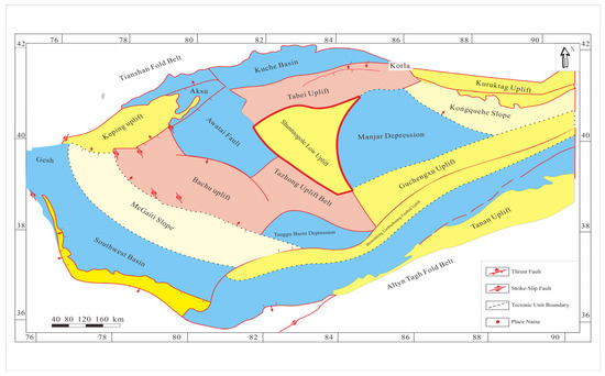
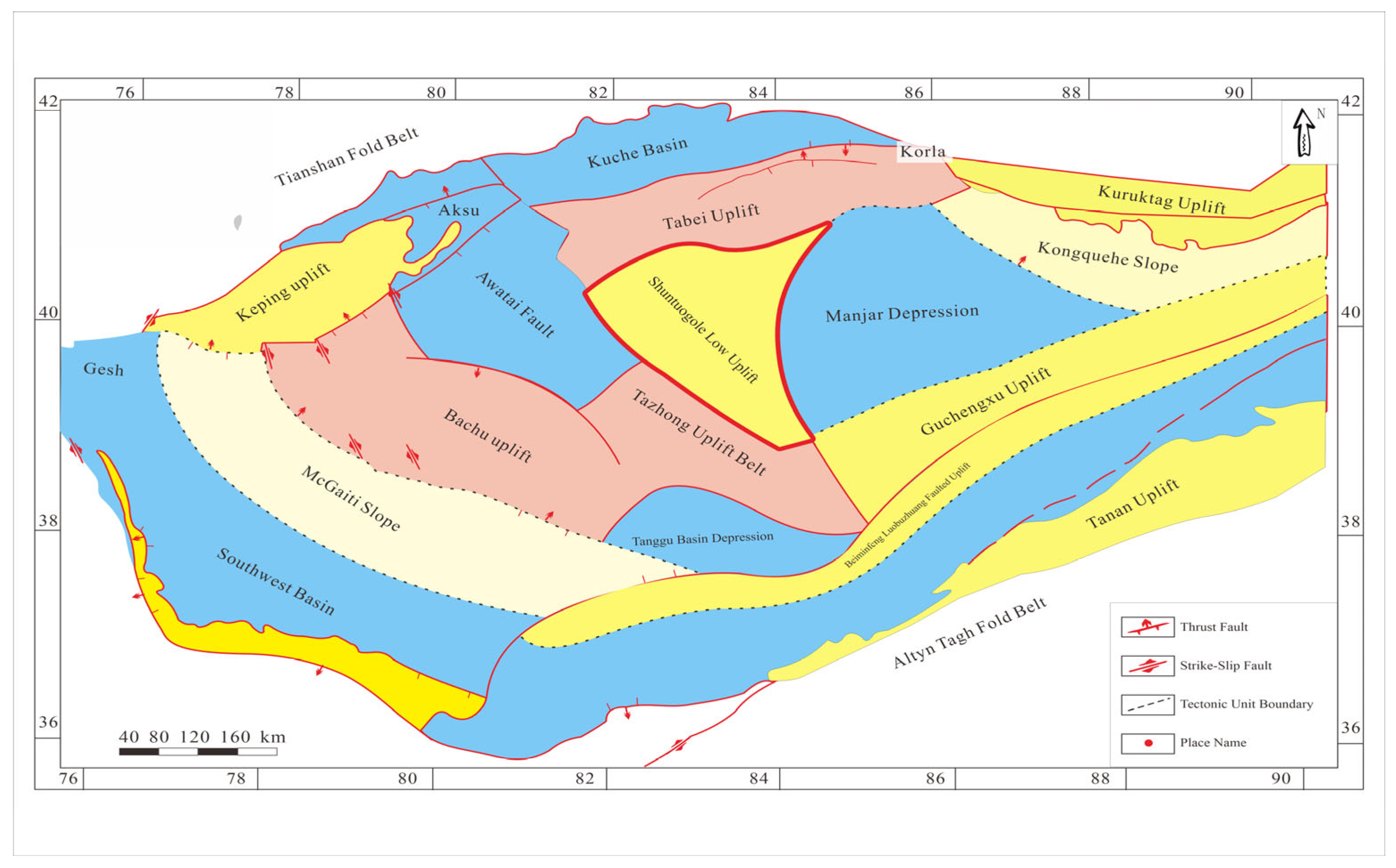
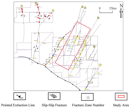
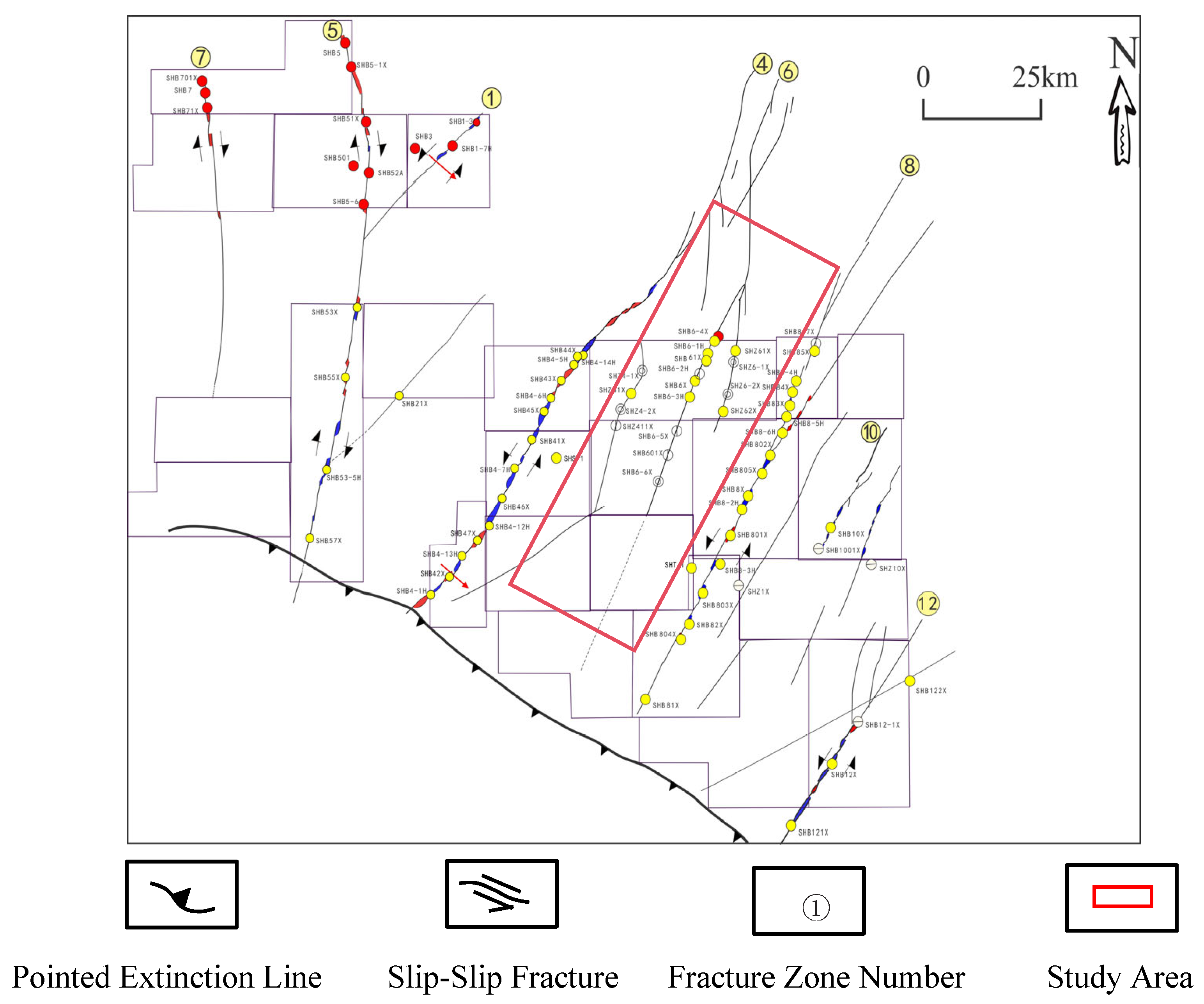
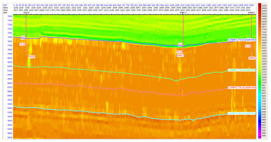
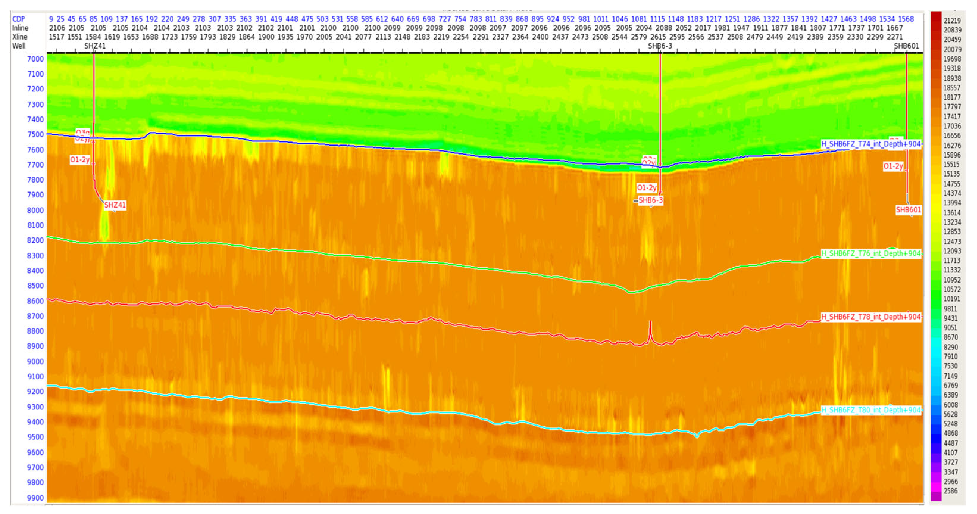
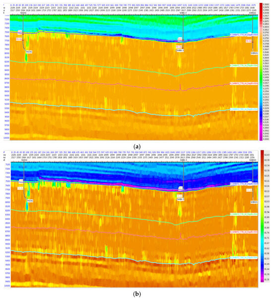
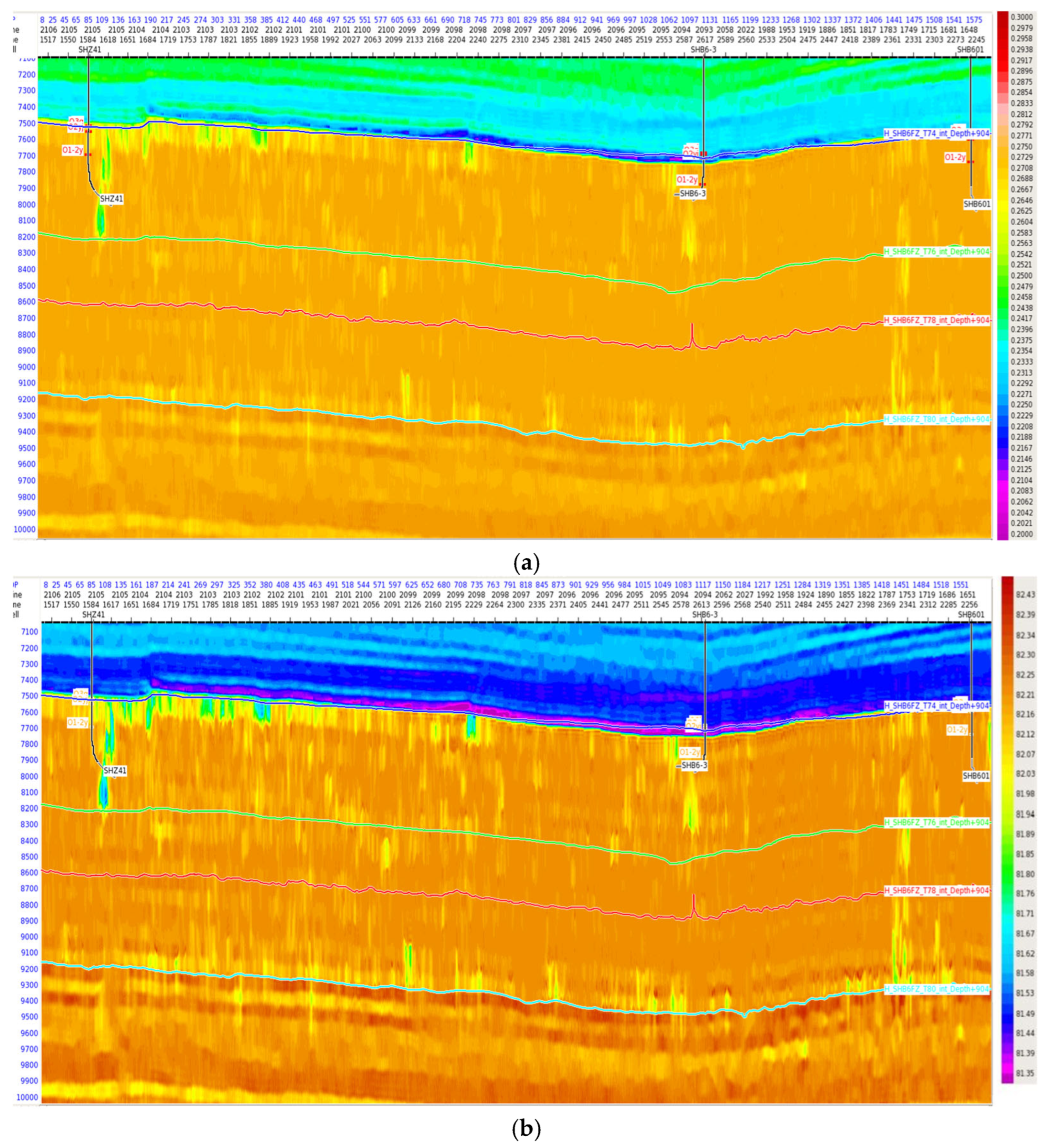
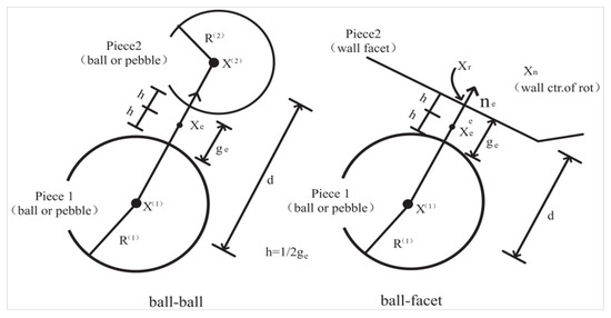
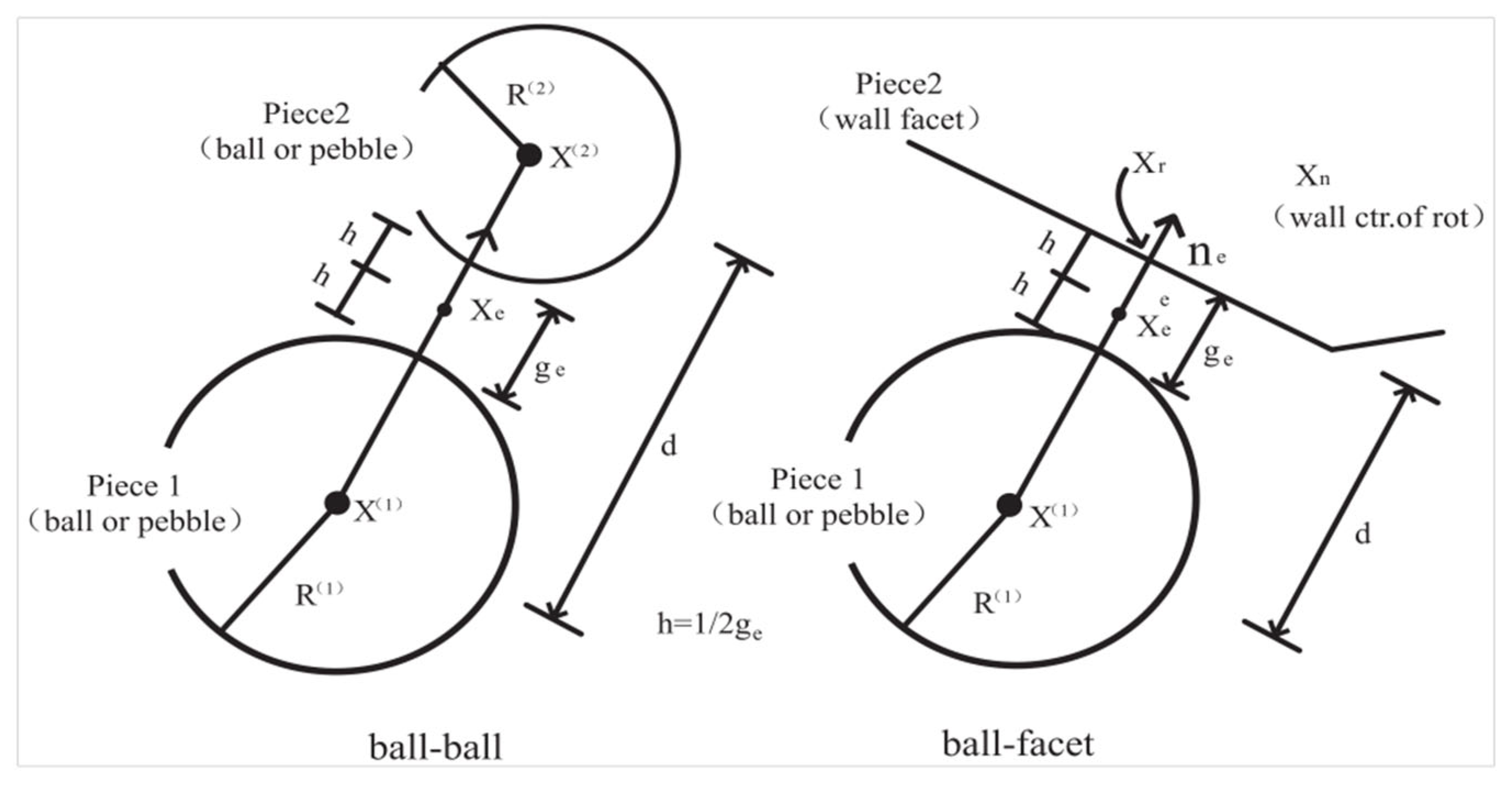
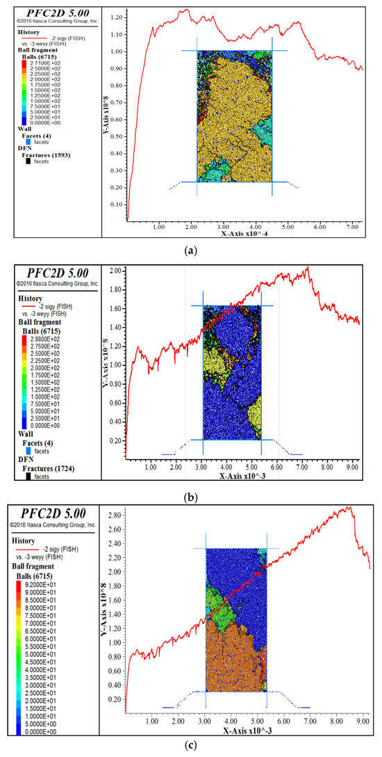
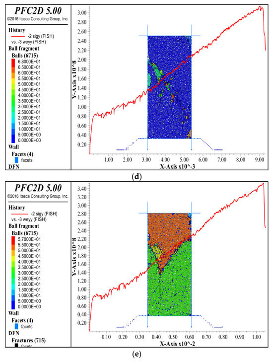
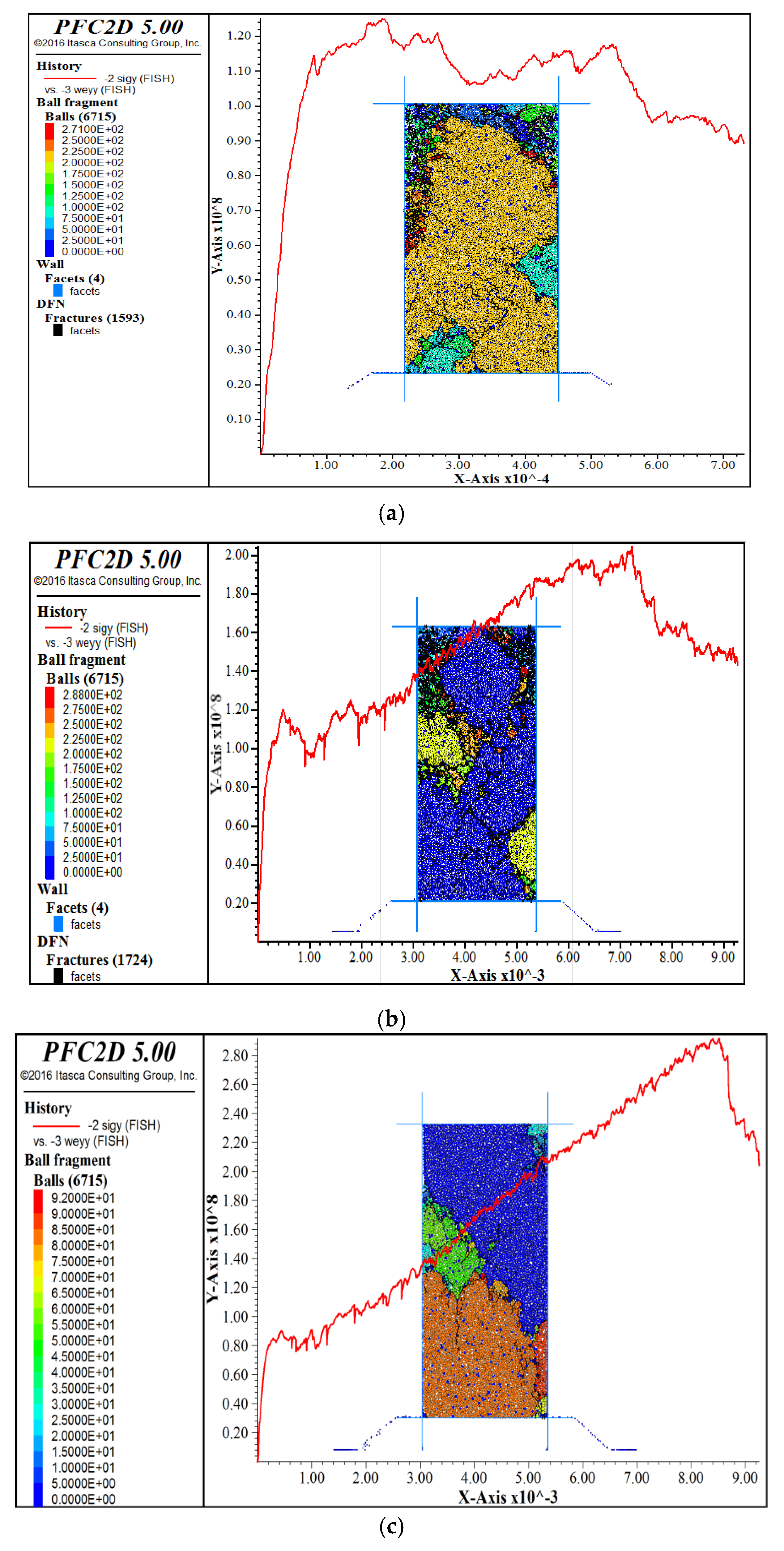
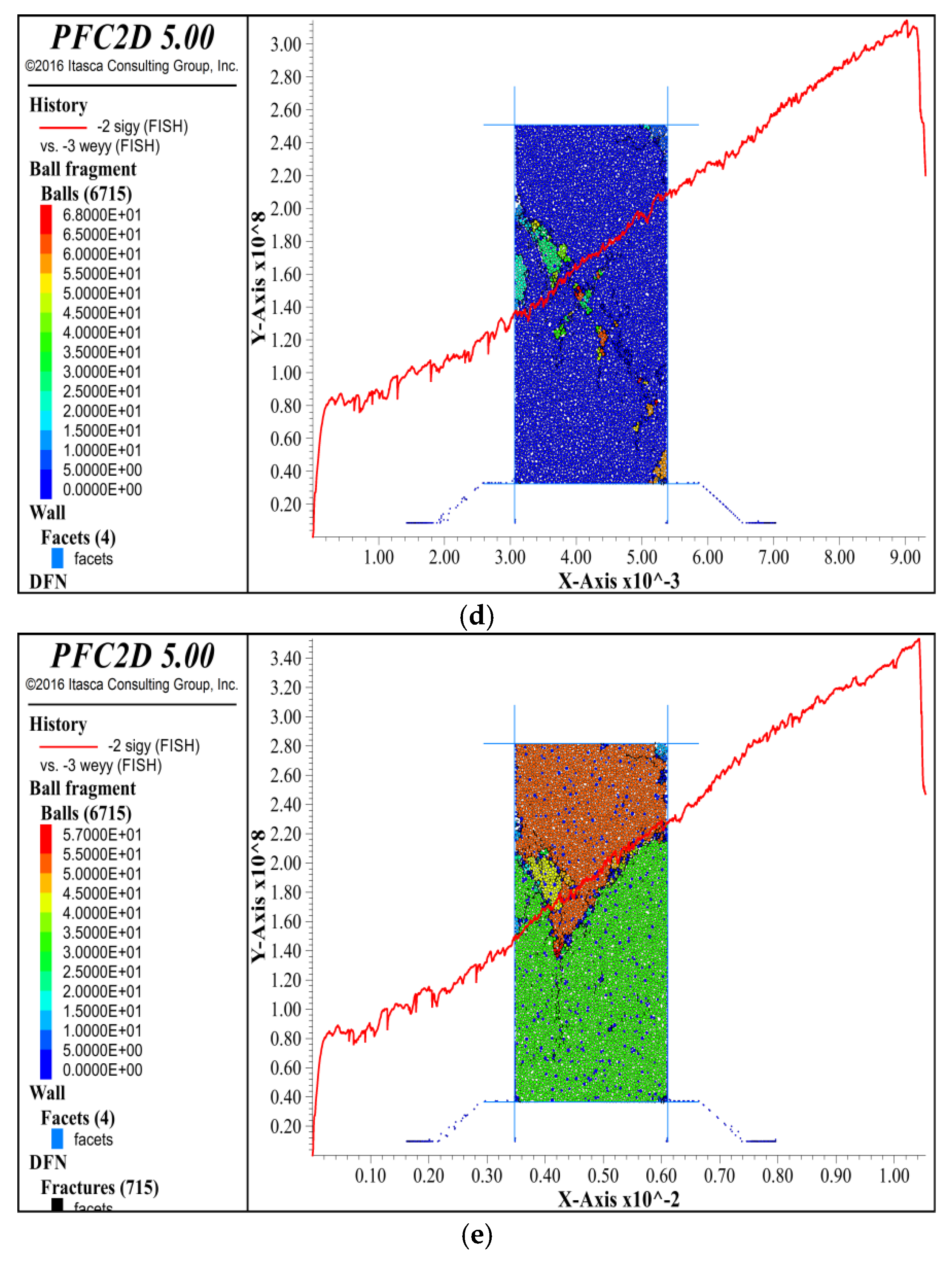
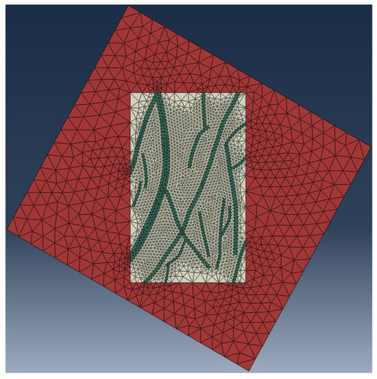
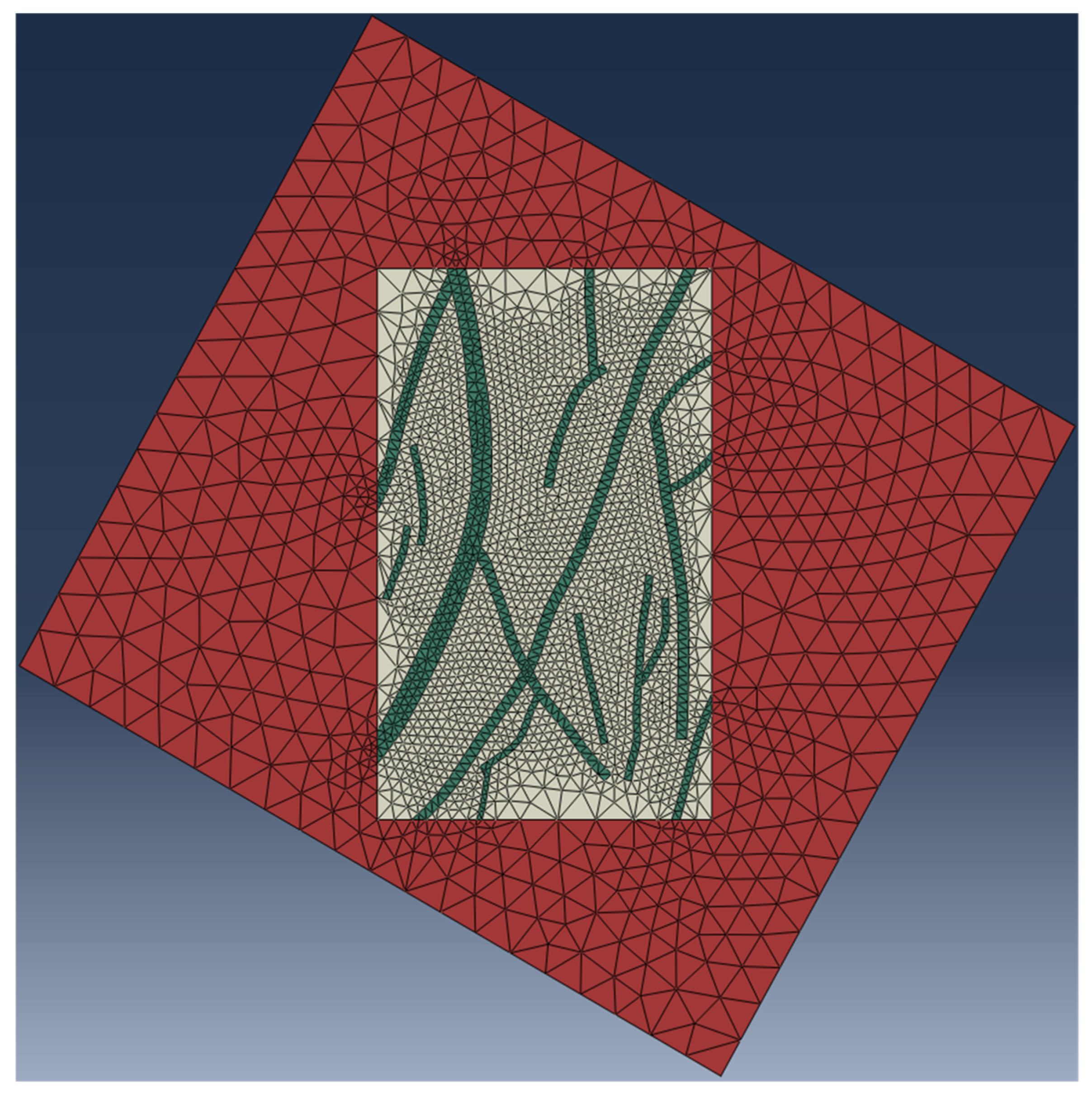
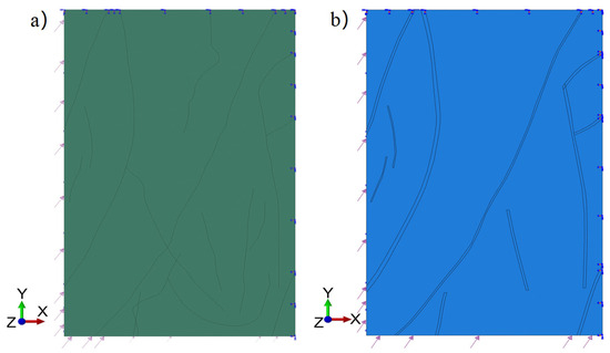
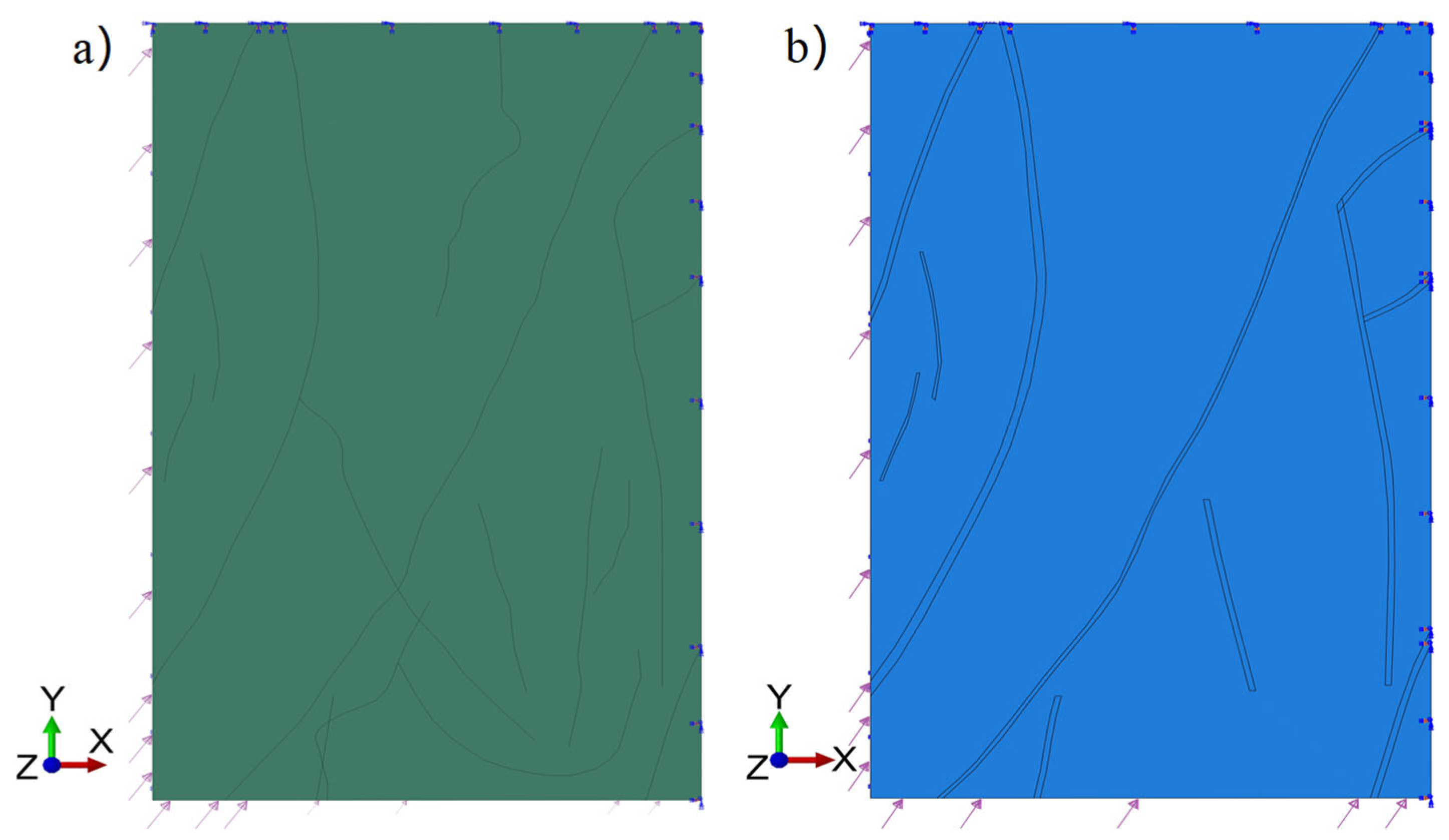
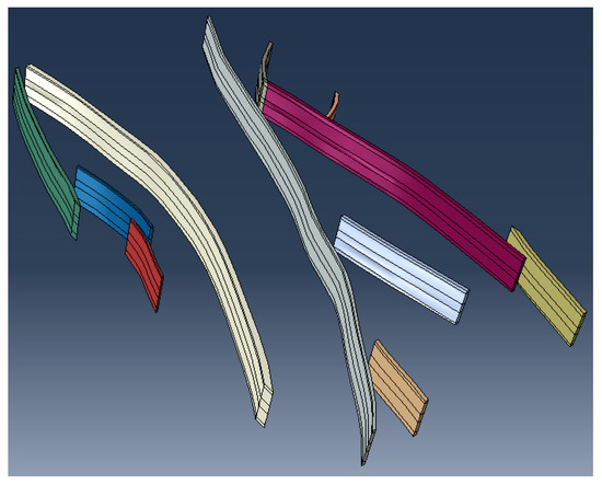
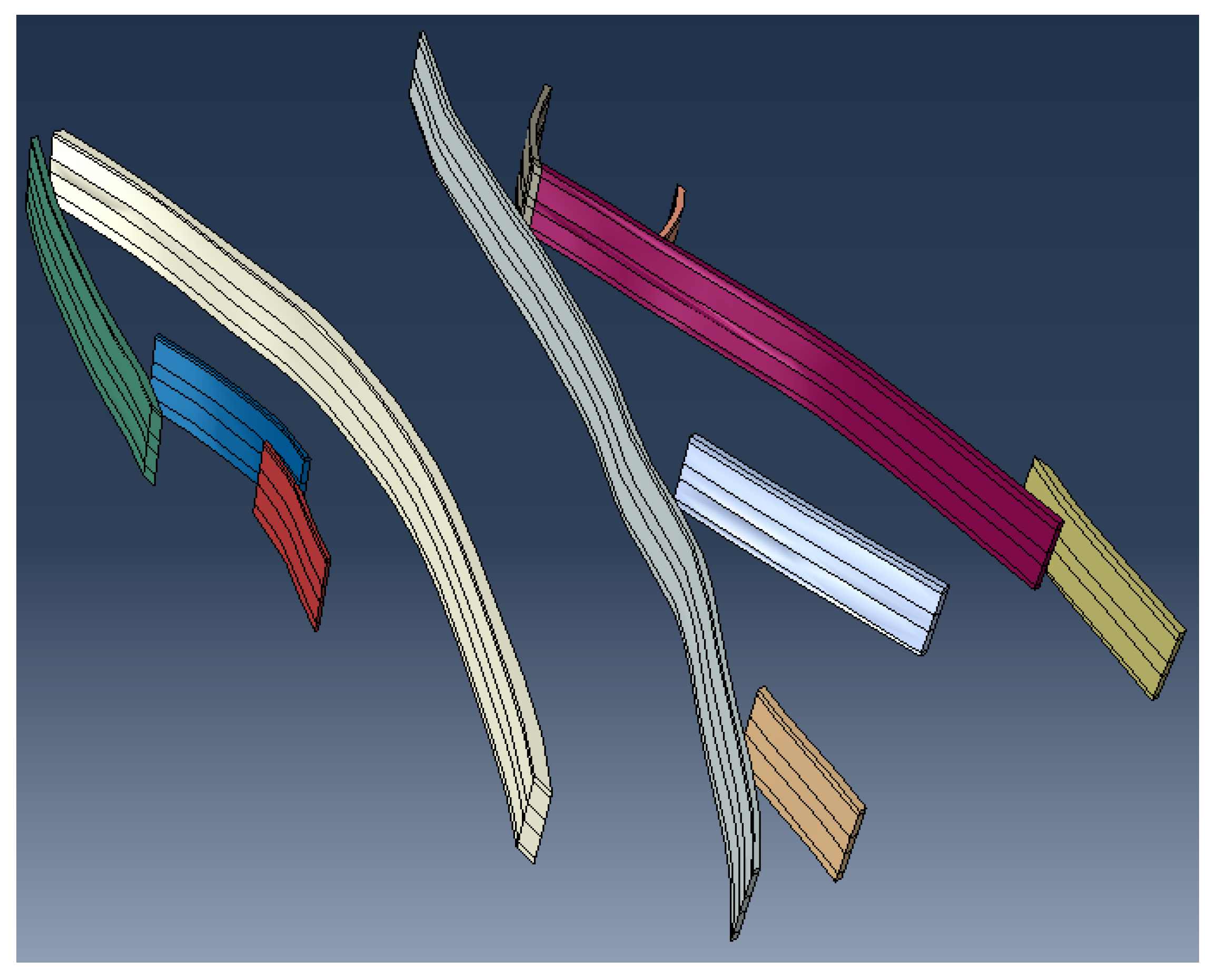
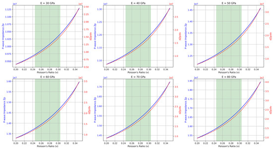
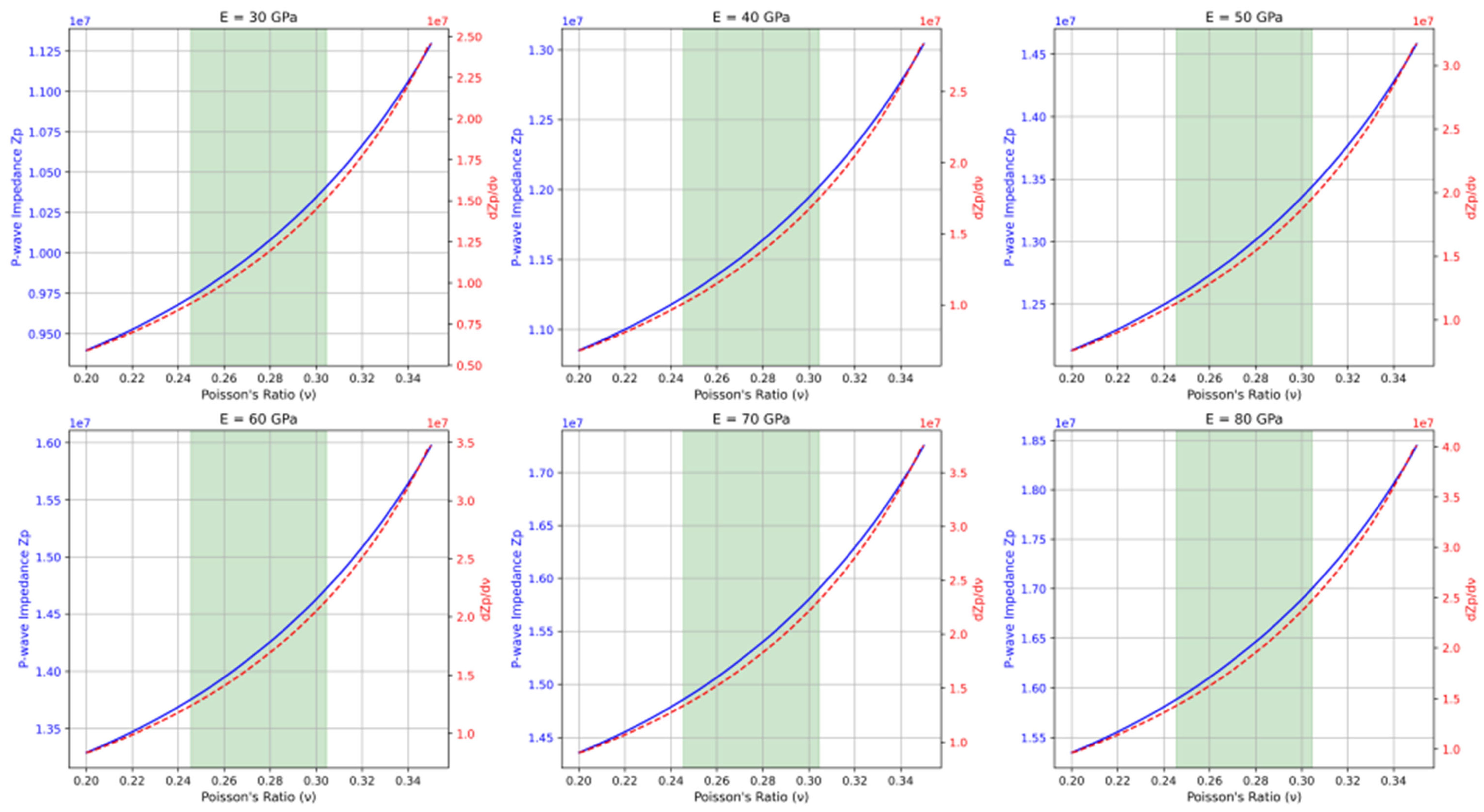
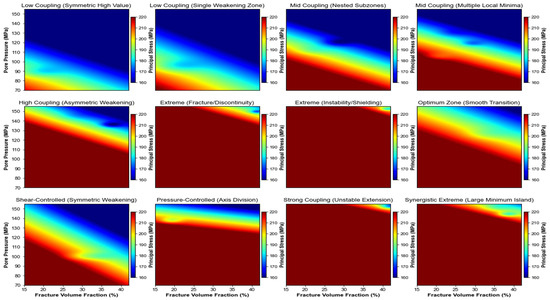
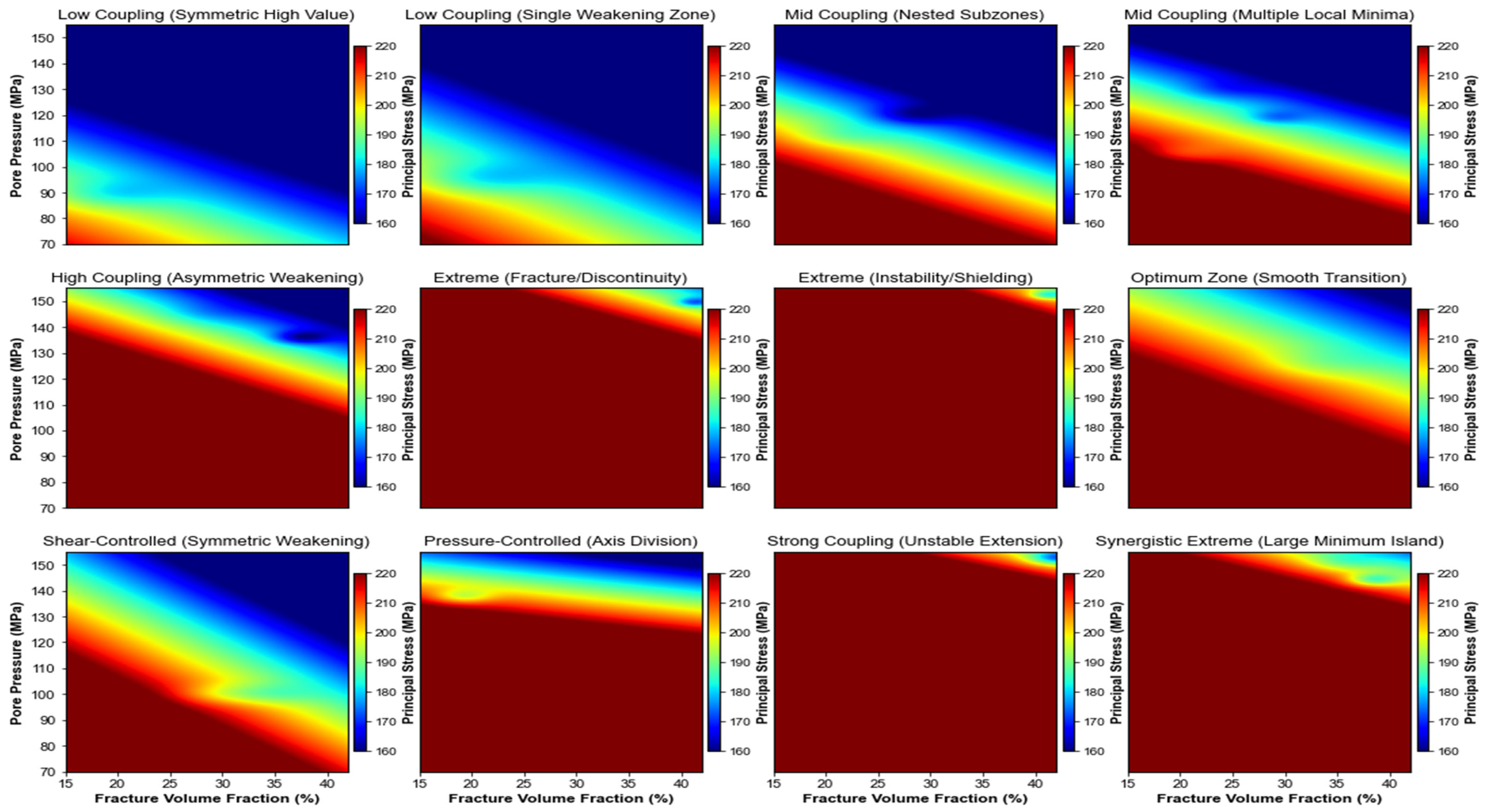
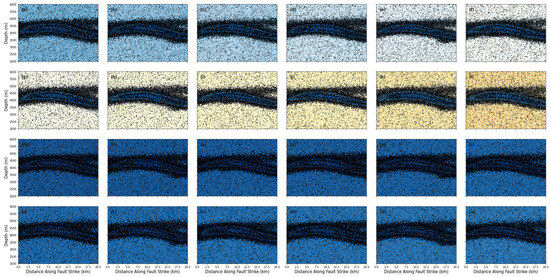
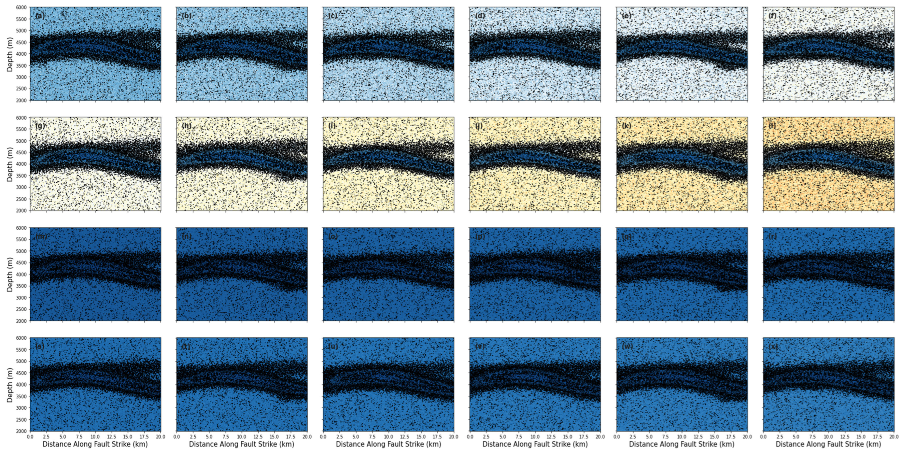
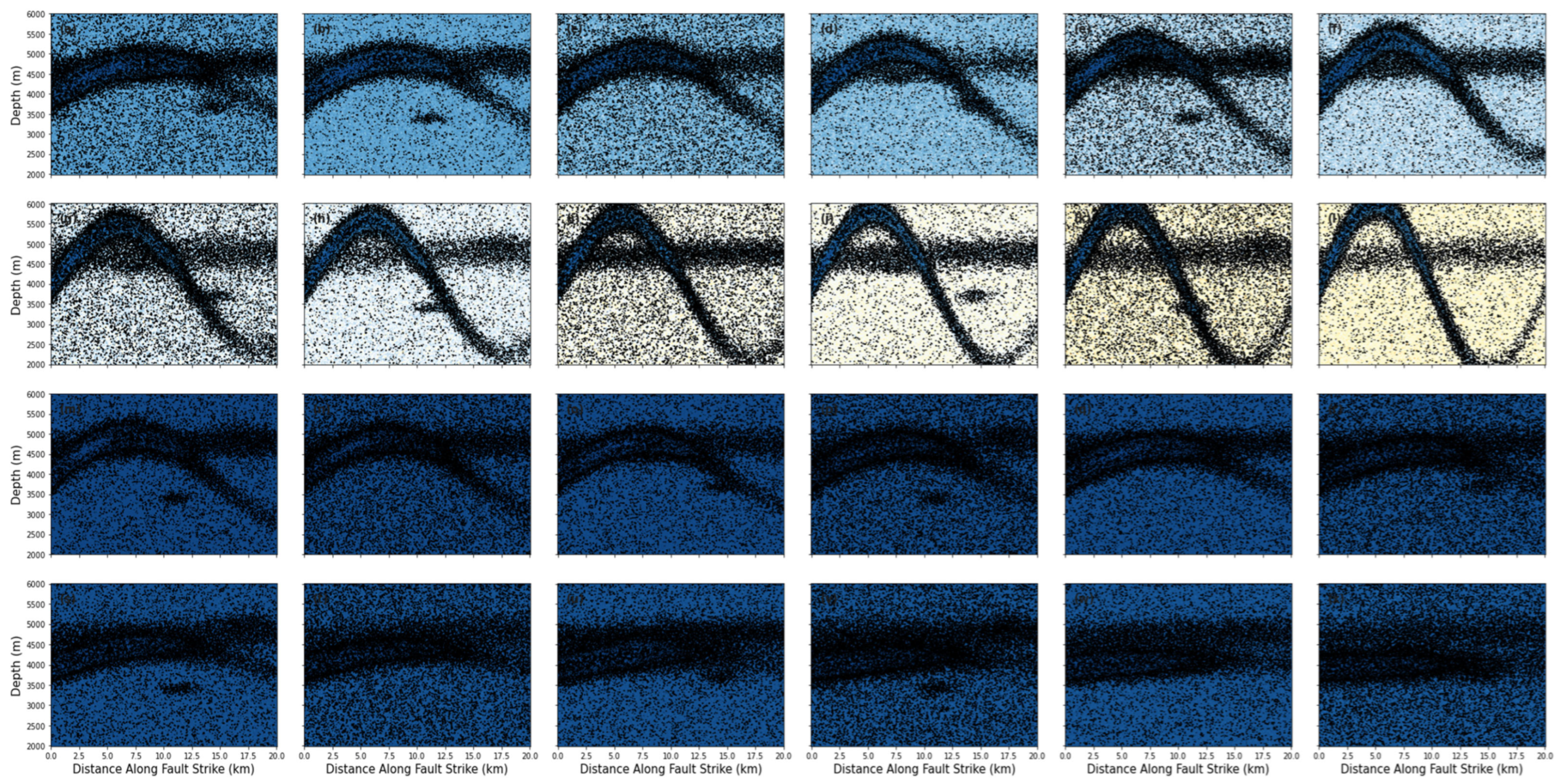
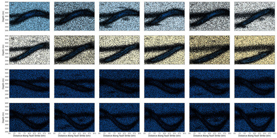
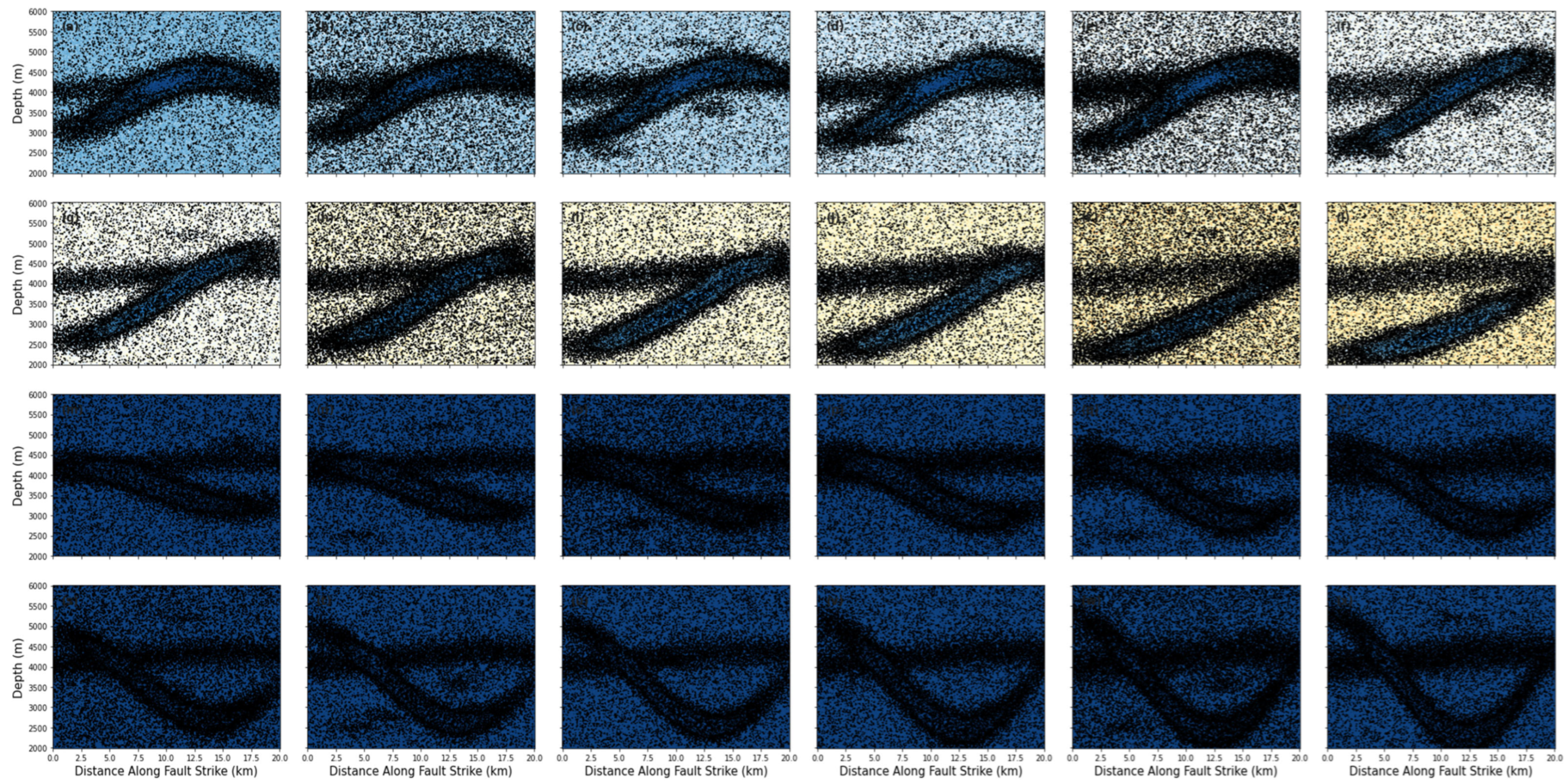
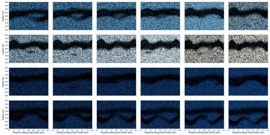
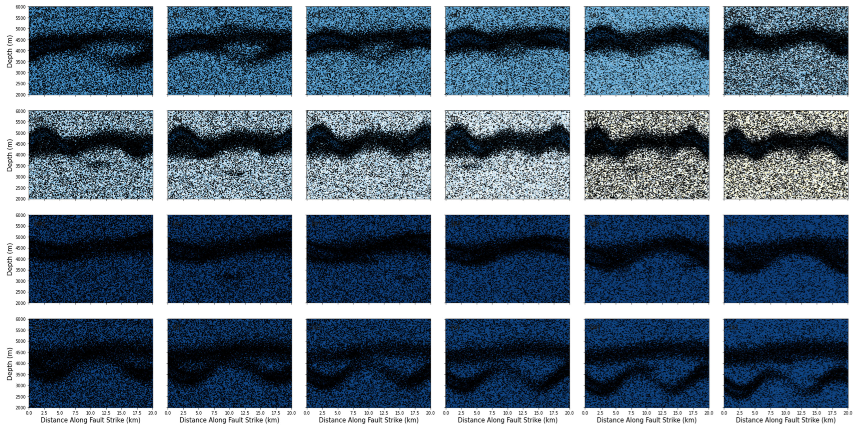
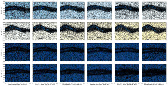
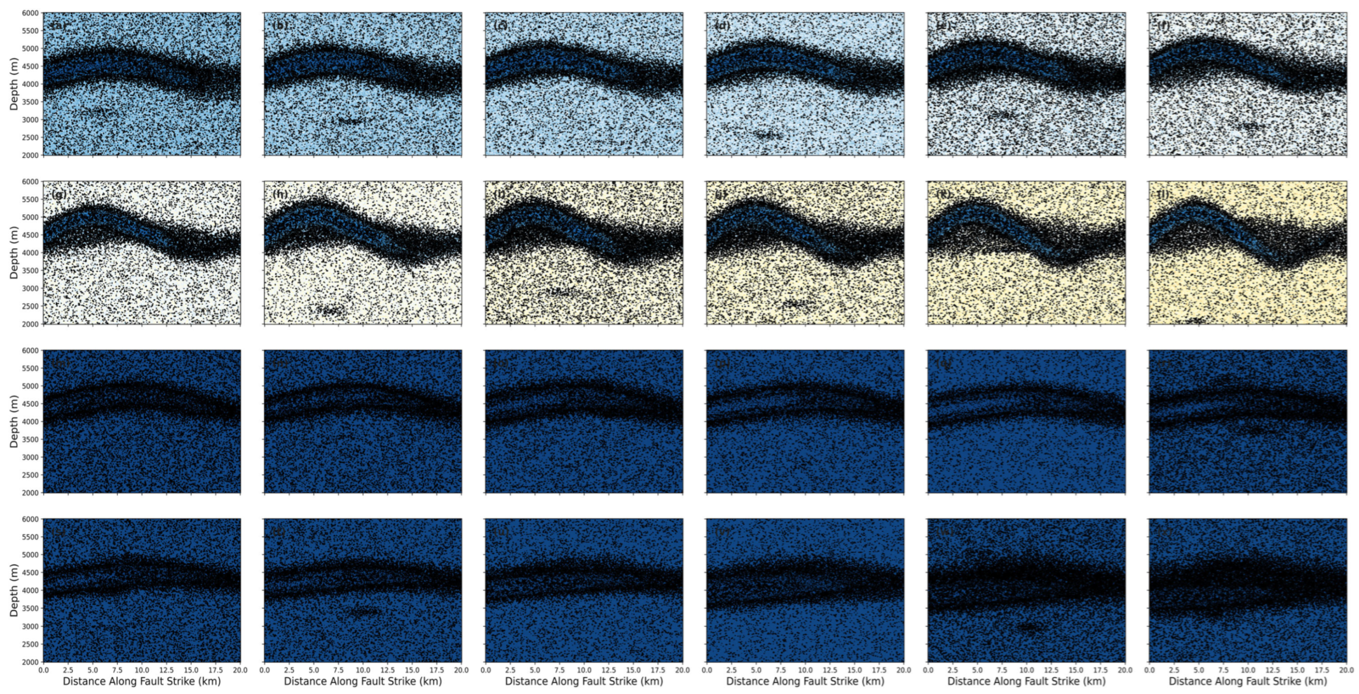
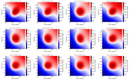
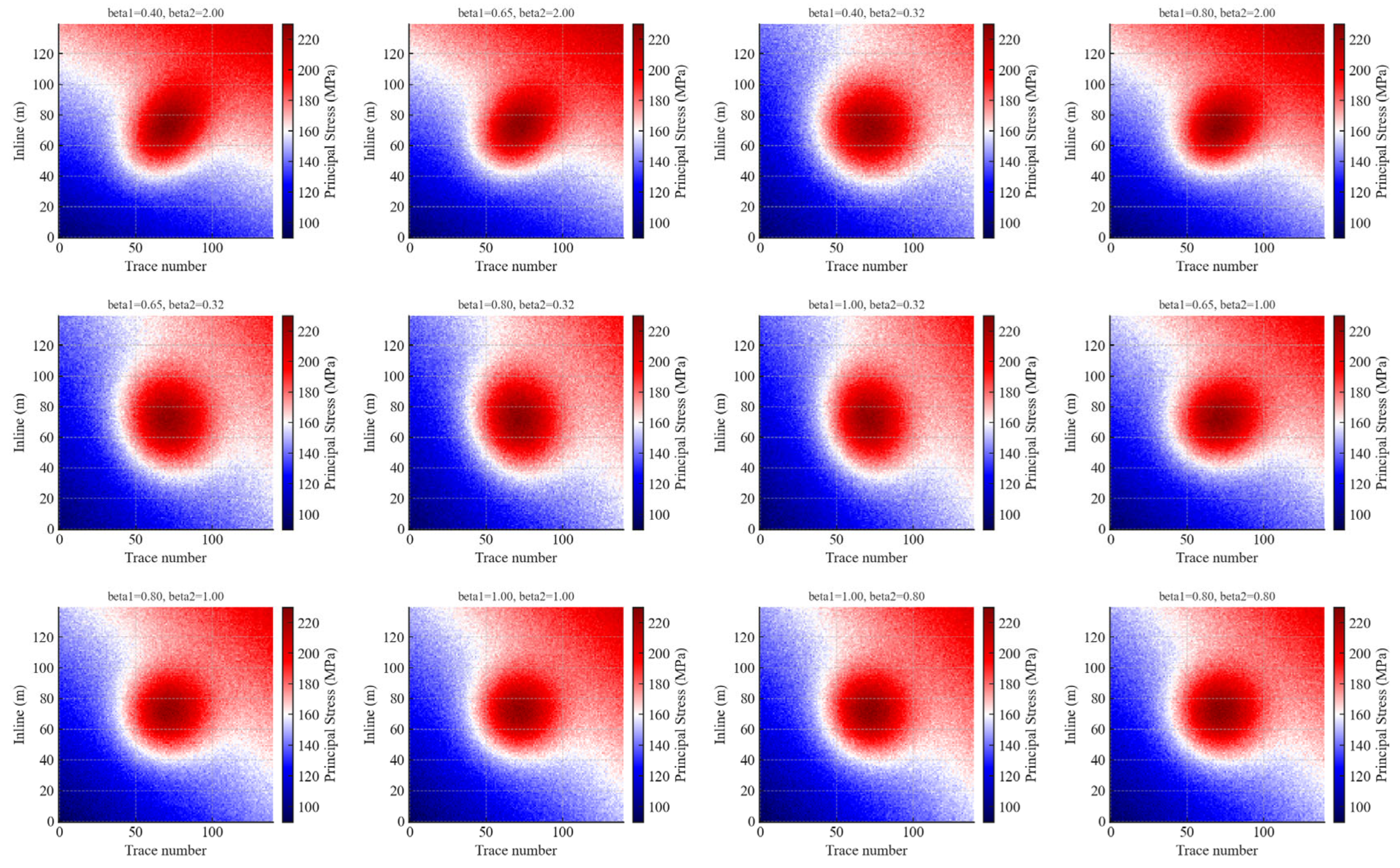
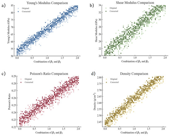
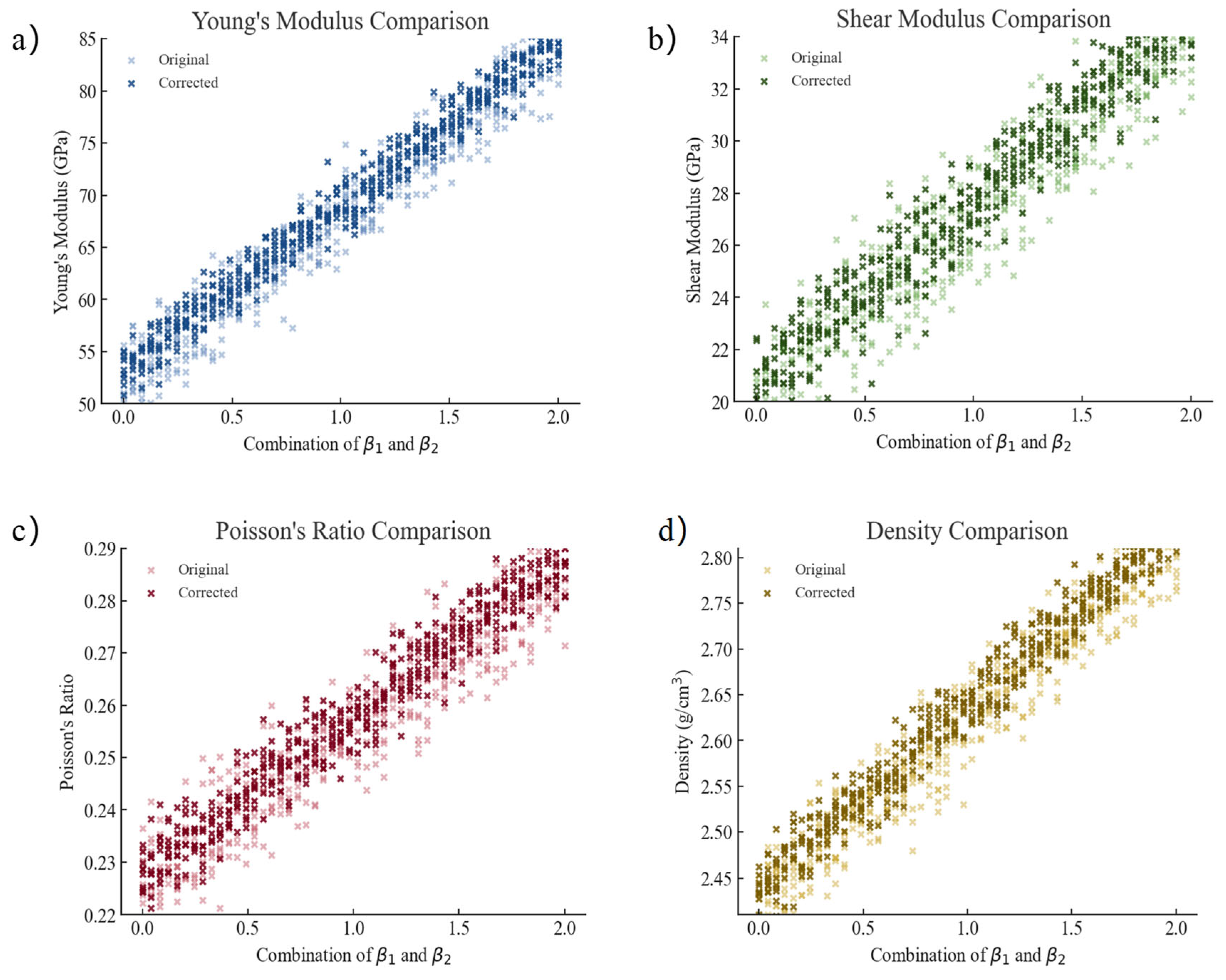
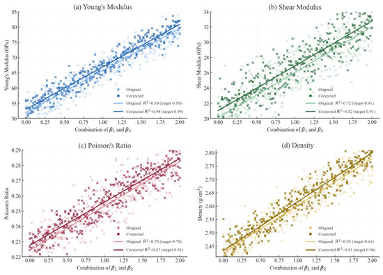
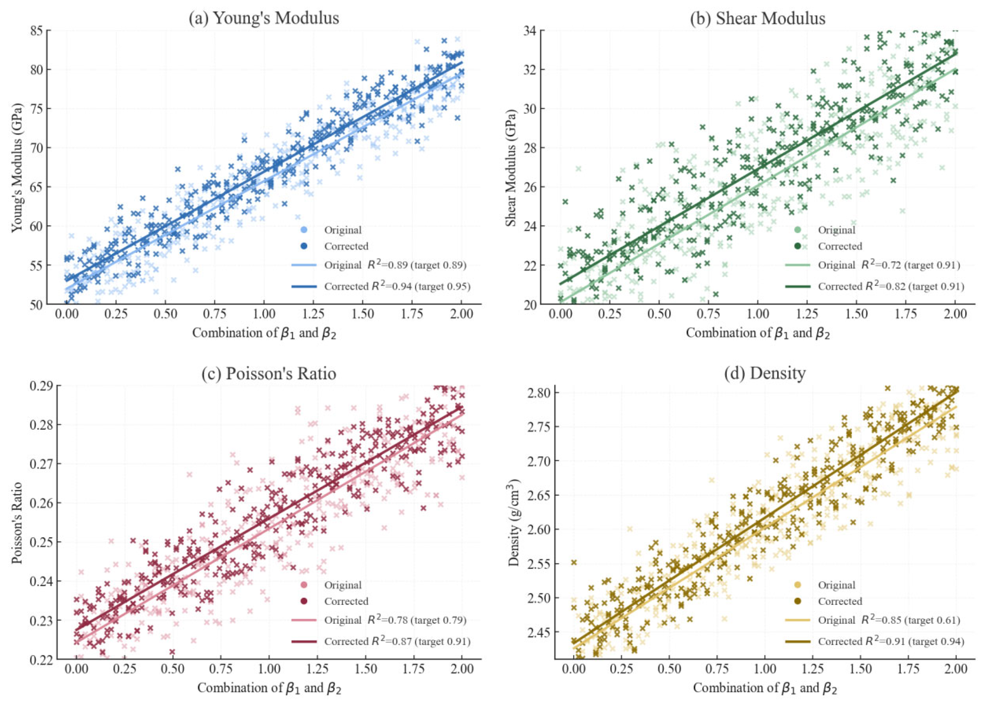
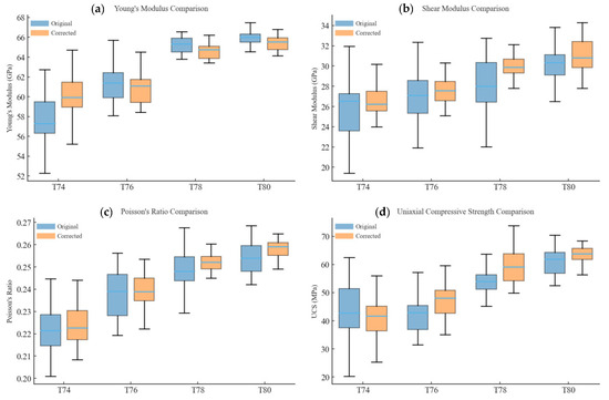
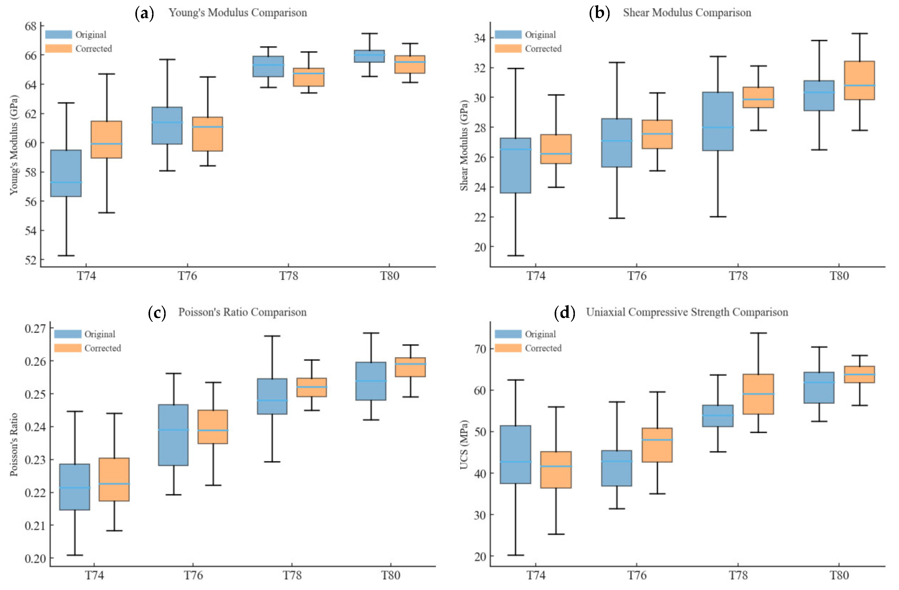
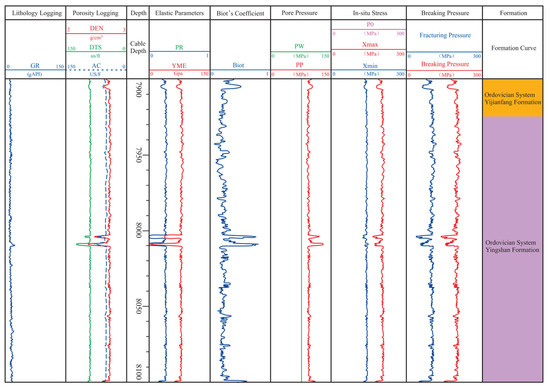
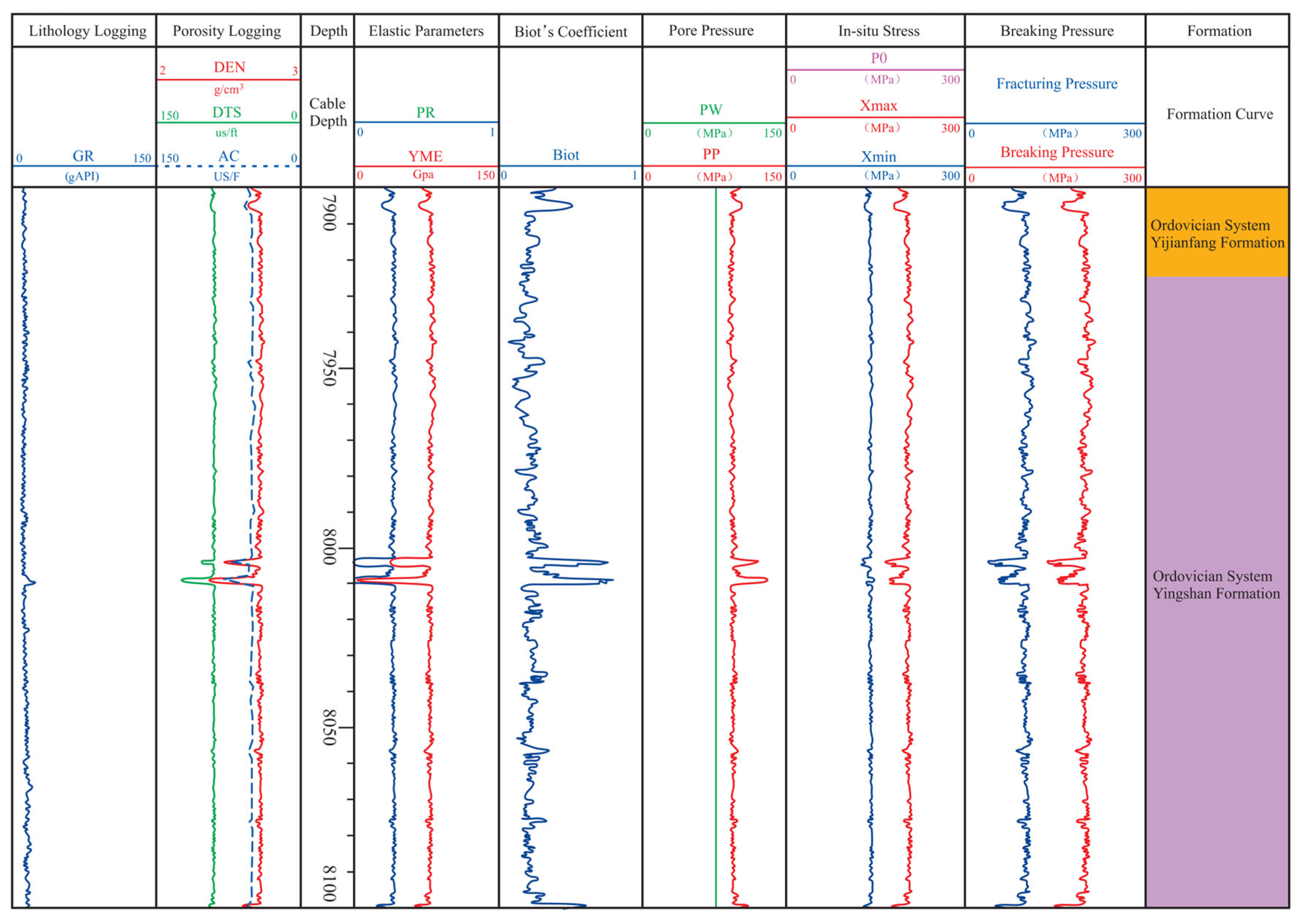
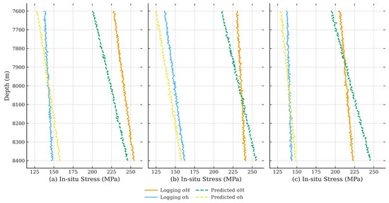
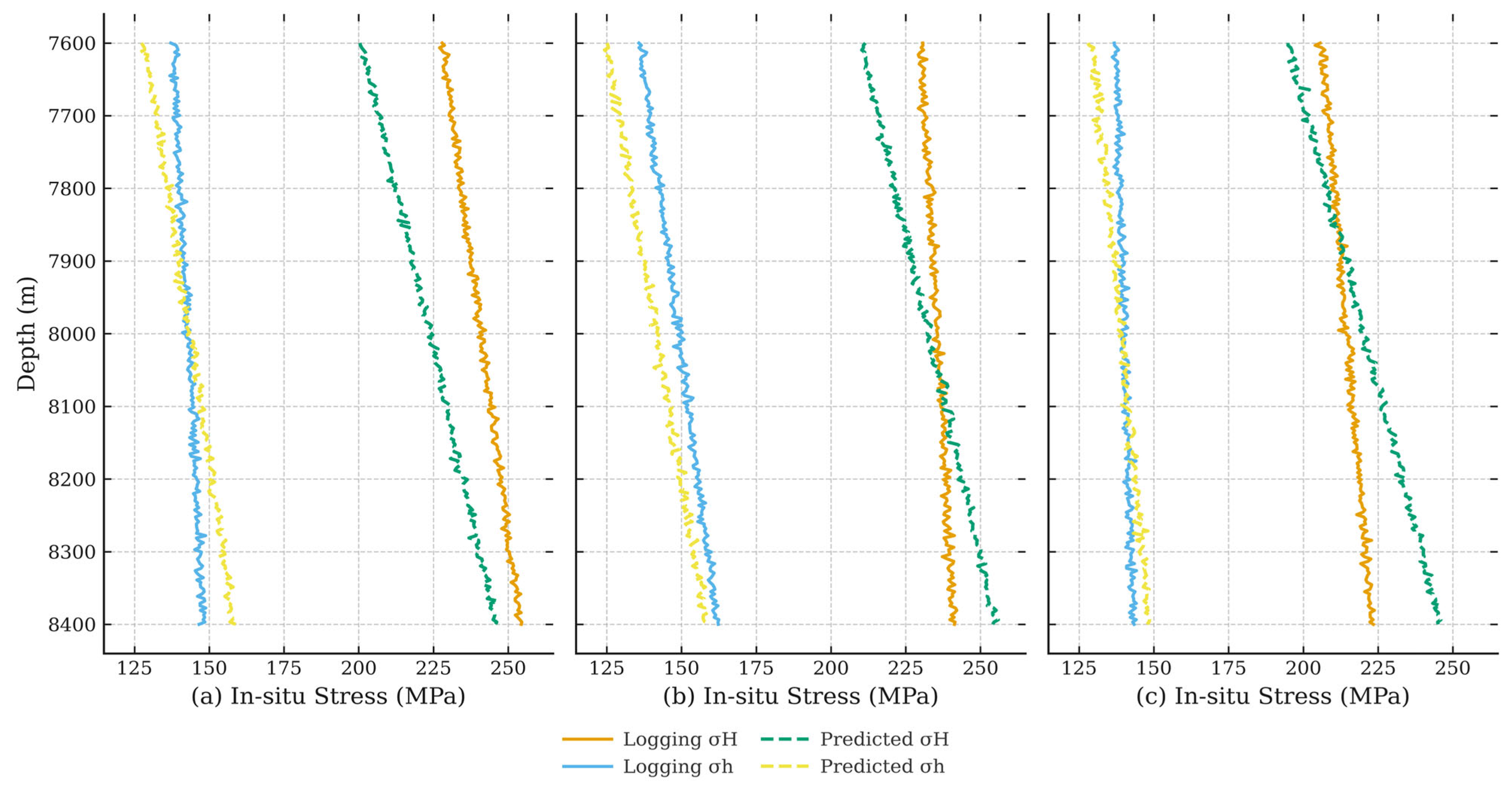
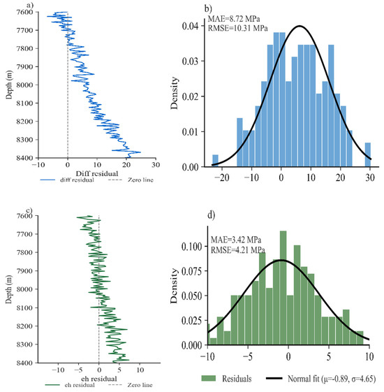
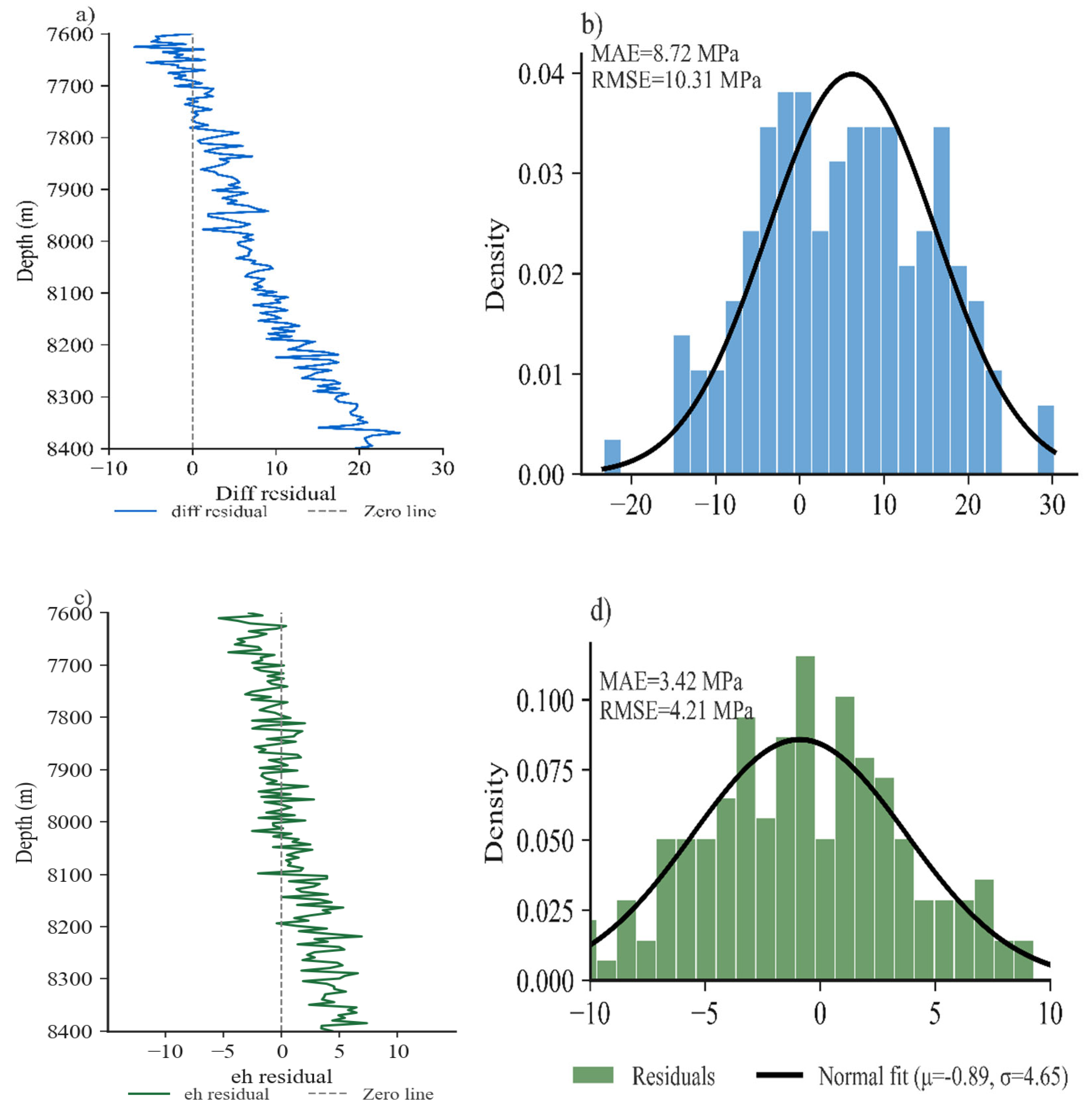
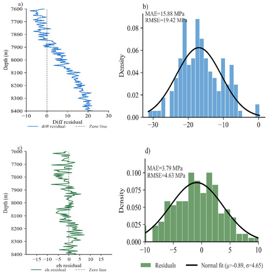
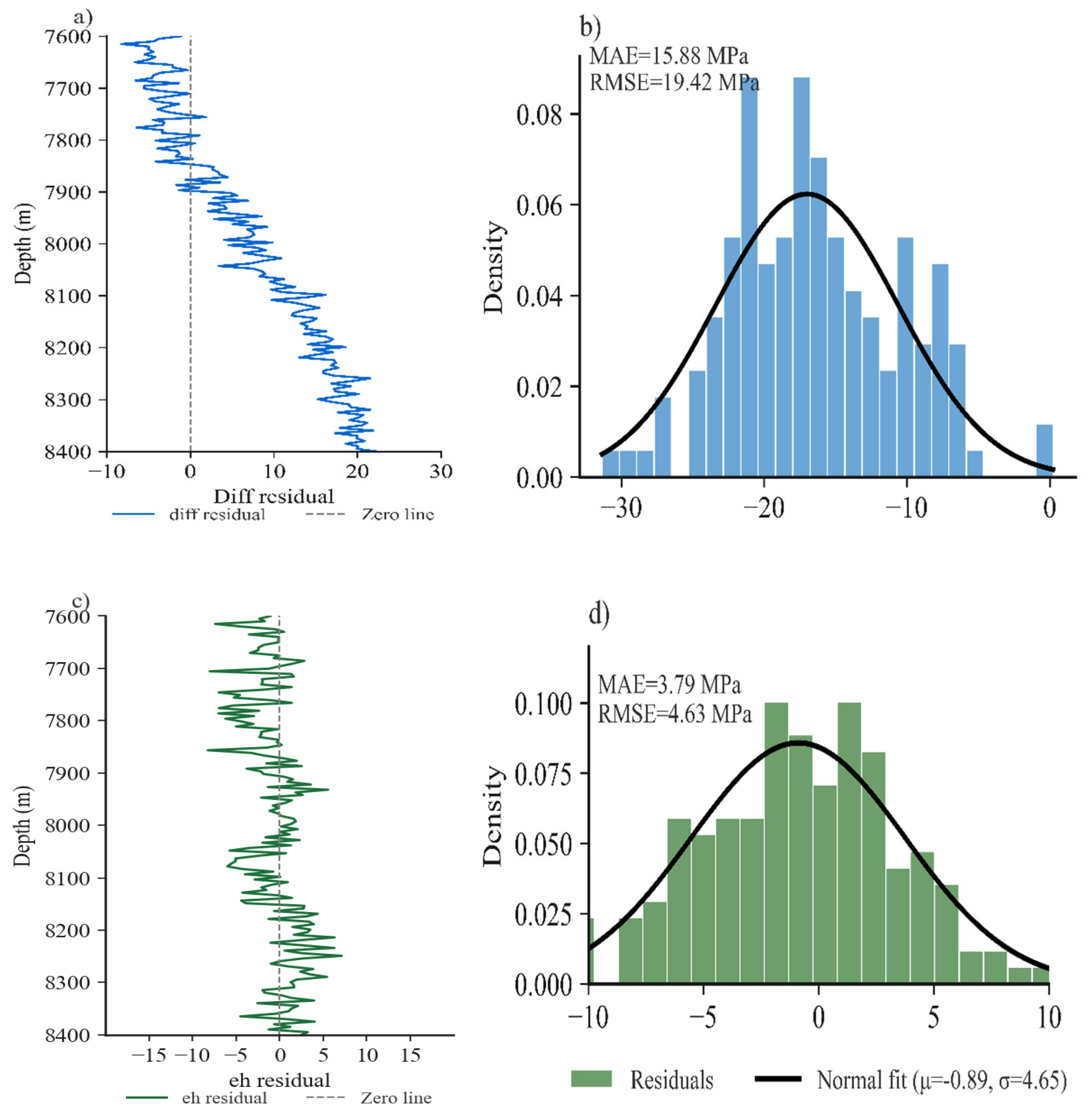
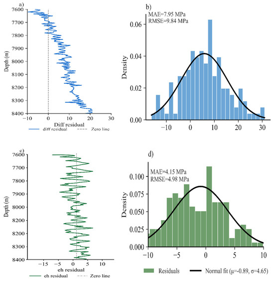
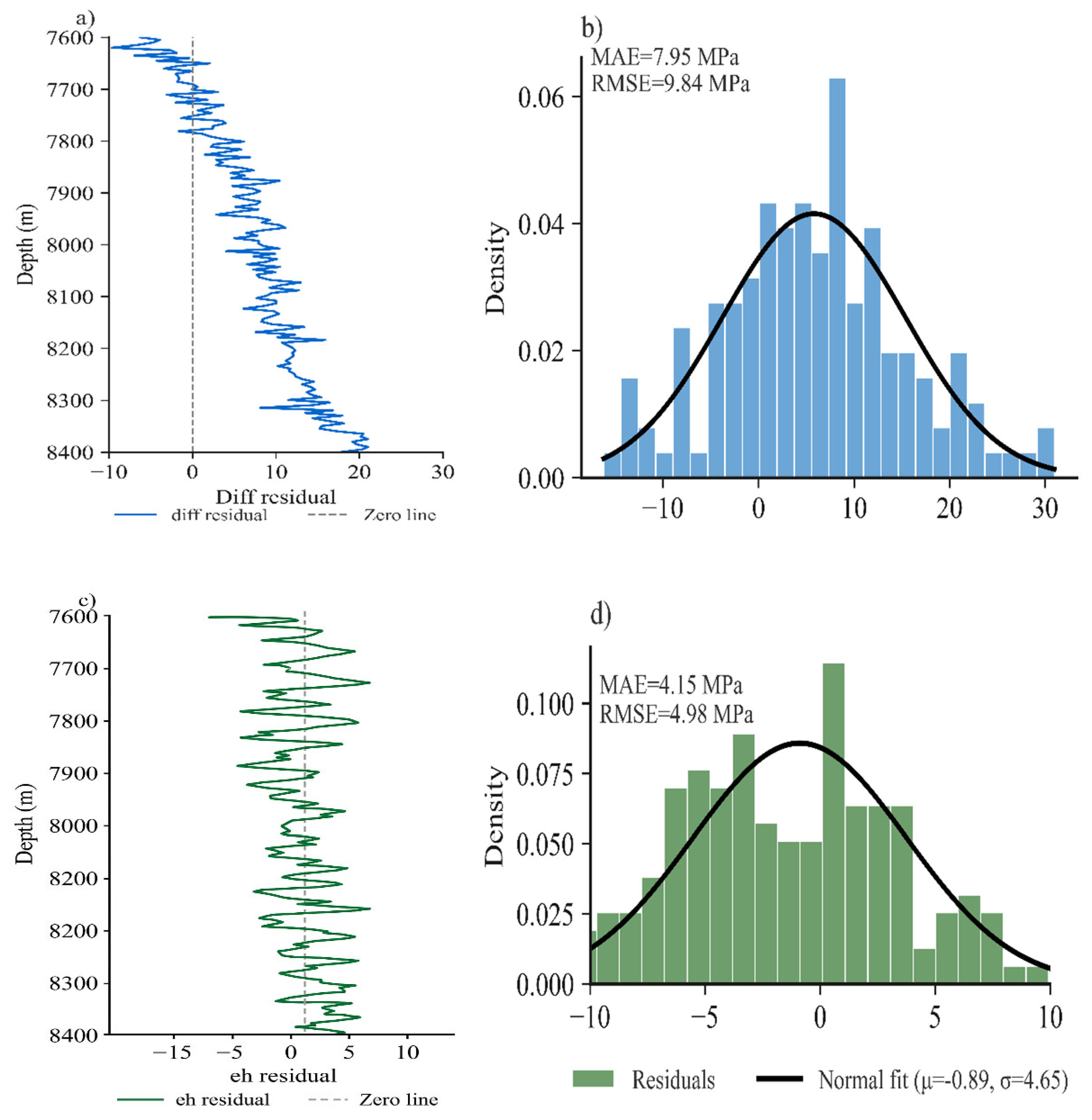
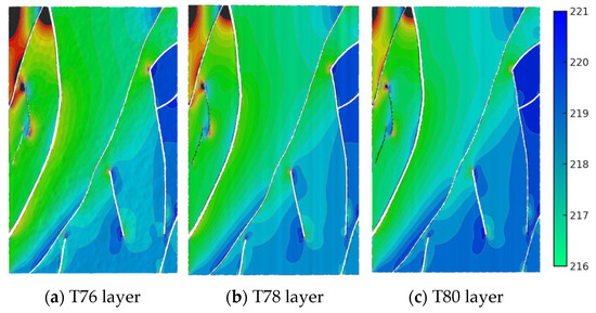
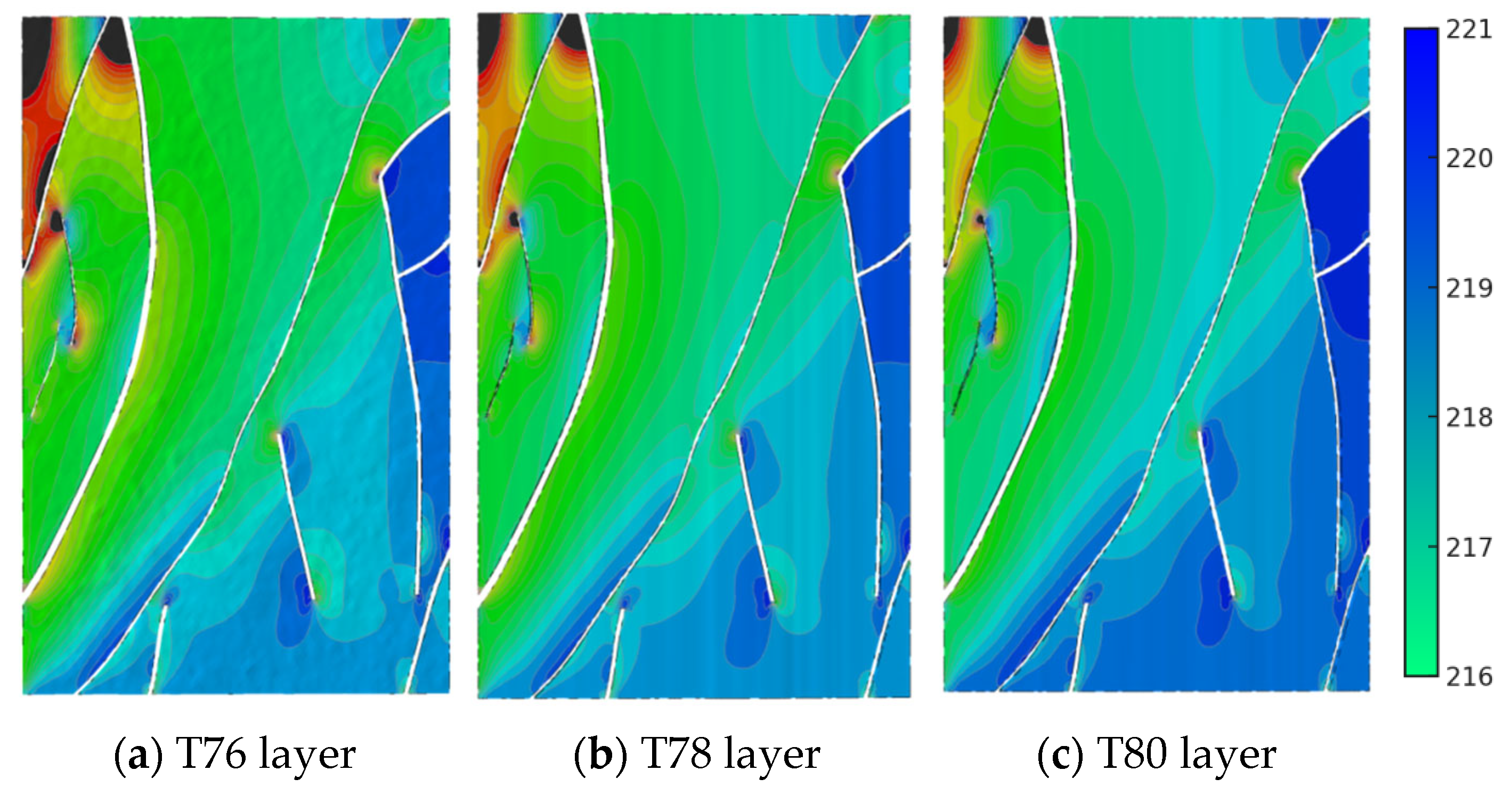
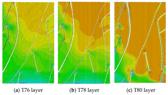
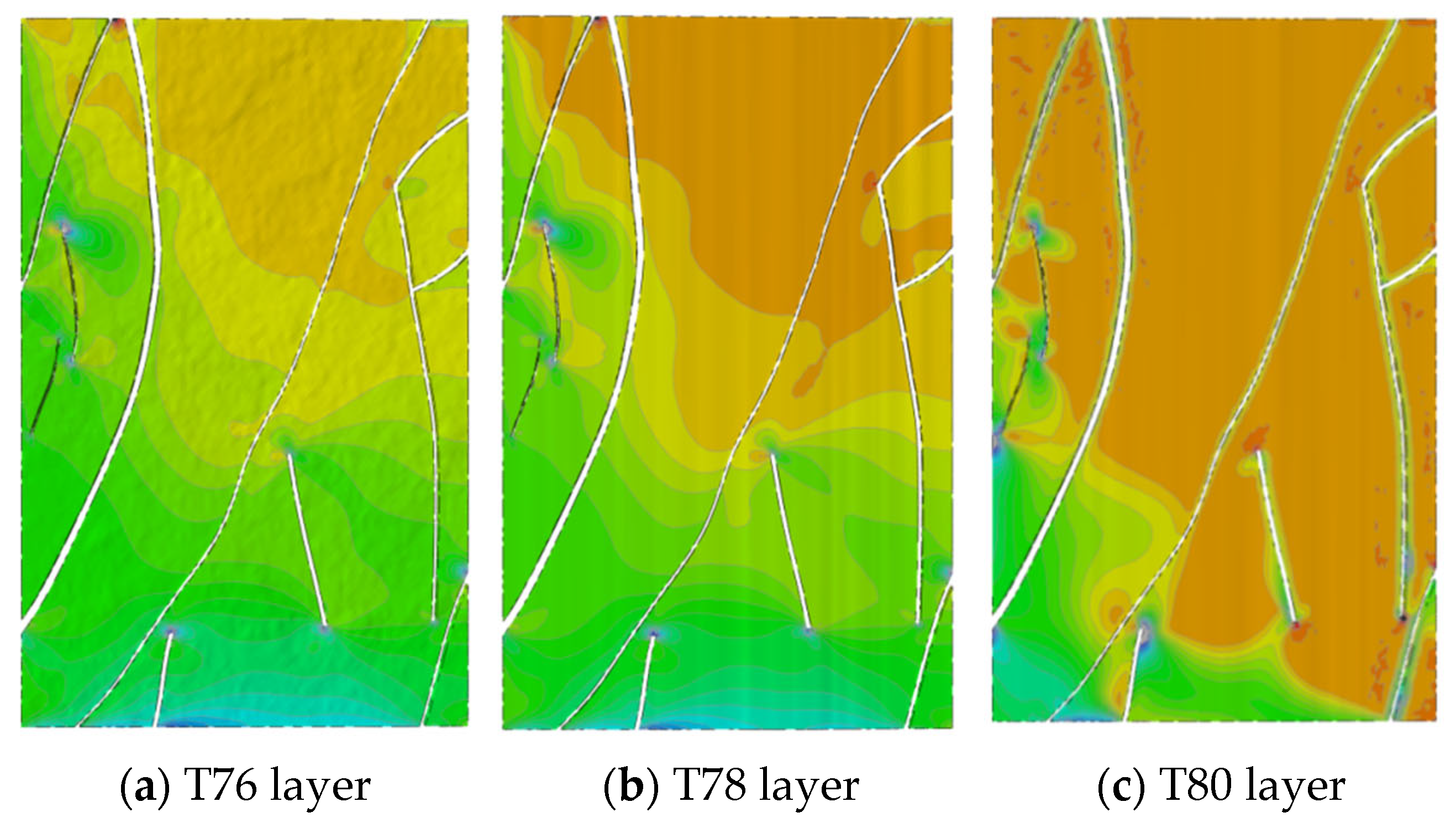

Disclaimer/Publisher’s Note: The statements, opinions and data contained in all publications are solely those of the individual author(s) and contributor(s) and not of MDPI and/or the editor(s). MDPI and/or the editor(s) disclaim responsibility for any injury to people or property resulting from any ideas, methods, instructions or products referred to in the content. |
© 2025 by the authors. Licensee MDPI, Basel, Switzerland. This article is an open access article distributed under the terms and conditions of the Creative Commons Attribution (CC BY) license (https://creativecommons.org/licenses/by/4.0/).