Meta-Learning Enhanced Random Forest Ensemble for Short-Term Oil Well Production Forecasting

Abstract

Accurate short-term oil production forecasting is critical for national energy security and strategic resource planning. However, in practice, the prevalent reliance on extensive daily production histories for training sophisticated models are often impractical. Consequently, a significant challenge lies in developing stable and precise forecasting models that utilize inherently limited monthly production data. To address this limitation, a meta-learning architecture is proposed to enhance the temporal representational capacity of ensemble random forests (RFs) for short-term production prediction. Specifically, three innovative meta-ensemble frameworks are introduced and evaluated: (1) independent RF base learners integrated with RF meta-learners, (2) time-embedded sequential RF base learners integrated with RF meta-learners, and (3) time-embedded sequential RF base learners with a fully connected network (FCN) meta-learner. Rigorous validation on a substantial dataset comprising 2558 wells from the Daqing Oilfield, each with fewer than 70 months of available production data, demonstrates the superior efficacy of the meta-learning-enhanced ensembles. Experimental results show that these frameworks significantly outperform established production forecasting methods, including CNN-BiLSTM models that are recognized for their inherent tempo ral correlation capture. The proposed approach achieves a notable 22.3% reduction in Mean Absolute Error (MAE) and a 17.8% improvement in root mean squared error (RMSE) for three-month-ahead forecasts, underscoring its potential for robust production forecasting under data scarcity.

1. Introduction

Economic development continues to be the dominant theme in global progress. Oil, commonly termed “black gold”, is undeniably the most vital resource foundation for modern economic development [1]. However, as fossil fuels are inherently non-renewable, accurate oil production forecasting becomes essential for enabling efficient resource development [2]. In particular, short-term production forecasting (e.g., predicting the next 3 months using easily available monthly data) is crucial for enabling real-time operational adjustments, optimizing extraction efficiency, and minimizing economic losses. In contrast, long-term forecasts (e.g., annual or multi-year projections) based on limited monthly data suffer from accumulating uncertainties and offer diminishing practical utility for guiding timely short-term production strategies. Despite its importance, achieving reliable short-term production prediction with monthly production history data remains a persistent and complex engineering challenge, primarily due to the highly non-linear and non-stationary characteristics of production data, which are influenced by complex subsurface flow dynamics, varying well conditions, and changing production strategies.

To address the challenge of oil production forecasting, three primary methods have been proposed: numerical simulation, statistical modeling, and data-driven machine learning approaches [3]. Numerical simulation-based methods utilize sophisticated reservoir simulators to accurately forecast future production by explicitly modeling the movement dynamics of subsurface [4,5]. Although physically insightful, these methods typically entail prohibitively high computational and temporal costs. Moreover, the forecasting accuracy of these models is always unstable due to the inherent uncertainties associated with subsurface reservoir characterization. To achieve more stable forecasting results, statistical-based empirical methods have been widely adopted. Among these, the established Arps decline model was developed to predict the production decline behavior [6,7], leveraging its consideration of reservoir drive mechanisms and reliance on historical production data. However, these models are largely semi-quantitative and fail to capture complex, localized temporal variations. To achieve quantitative forecasting, statistical methods such as the auto-regressive integrated moving average (ARIMA) algorithm have been utilized [8]. They rely on assumptions of stationarity that are often violated in real production settings, limiting their applicability for short-term dynamics. However, complex underground conditions and associated production strategies make it a highly non-stationary and non-linear problem of oil production forecasting.

Given these limitations, machine learning (ML) offers a promising direction for modeling the non-linear relationships inherent in production data to address the oil production forecasting challenge in a data-driven manner [9,10]. Earlier, classical machine learning methods such as artificial neural networks (ANN), support vector machine (SVM), random forests (RF), and extreme gradient boosting (XGBoost) were proposed to model the complex non-linear relationship between input features and production output [11,12]. Among them, tree-based ensembles, particularly RF and XGBoost, have consistently demonstrated superior performance in capturing complex, non-linear relationships [13,14,15]. While both are top-tier algorithms, RF offers distinct practical advantages for industrial/agricultural applications; its inherent robustness to noisy data and outliers minimizes overfitting and reduces preprocessing demands, and its model-agnostic feature importance analysis provides greater interpretability, which is crucial for fostering trust and providing insights in operational contexts [16,17]. Nonetheless, standard RF models do not inherently account for temporal dependencies, which restricts their accuracy in sequence-aware forecasting.

Recent advances have introduced deep learning models, including long short-term memory (LSTM) networks and transformer architectures, which excel at capturing temporal patterns. For instance, Song et al. [18] applied LSTM to forecast production in volcanic reservoirs; Kumar et al. [19] combined LSTM with autoregressive modeling; and Cao et al. [20] proposed an attention-based CNN-LSTM encoder–decoder. More recently, transformers have been explored for production forecasting [21,22]. However, such deep models require large volumes of high-frequency data for training and are prone to overfitting when applied to limited, monthly frequency production datasets—a common scenario in oilfield operations. This issue is exacerbated by the high variability in production profiles across different wells and reservoirs, making large models such as transformers less reliable for short-term forecasting under data scarcity [23,24].

To address the dual challenge of achieving high short-term forecasting accuracy with limited data while mitigating overfitting, we propose a meta-learning-enhanced random forest approach for short-term oil production forecasting. This method combines the inherent robustness and efficiency of RF with an improved capacity for modeling temporal dependencies, without requiring extensive datasets [25]. As illustrated in Figure 1, we introduce three specific meta-ensemble frameworks to operationalize this strategy. Figure 1a illustrates the overarching structure of the proposed meta-learning enhanced RF ensembles, while Figure 1b details the complete workflow for short-term production forecasting. In Figure 1b, RF-t + i represents the i-th base RF learner; MetaRF-t + i, T2-RF-t + i, and Tk-RF-t + i denote the i-th meta-RF learner at the corresponding meta-learning layer.

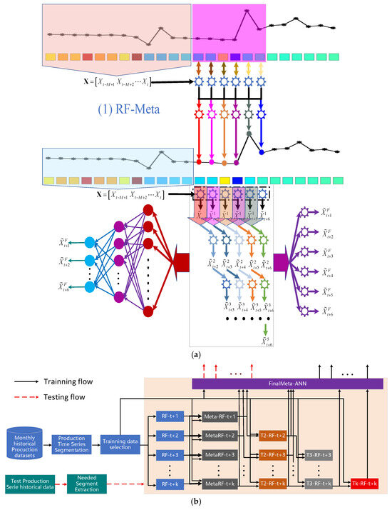
Figure 1. Illustration of the proposed meta-learning enhanced RFs ensemble methods for short-term production forecasting:(a) ensemble model framework; (b) detailed workflow with RRF-Meta-FCN as an example.

The remainder of this paper is organized as follows: The detailed description of the proposed method is given in Section 2. Additionally, Section 3 presents the experimental setup and the corresponding detailed discussion. Finally, Section 4 summarizes the key findings and suggests potential directions for future research.

2. Methodology

2.1. Random Forest

Building upon random subspace theory and ensemble learning techniques, the random forest algorithm integrates multiple decision trees in a bagging ensemble [26,27,28]. This versatile machine learning method is applicable to classification and regression tasks across various domains with highly competitive performance. Specifically, the RF algorithm constructs multiple decision trees following the classification and regression trees (CART) model [29]. The main structure of the RF algorithm is shown in Figure 2. For a given regression training dataset: D = {(x₁,y₁),(x₂,y₂),···,(x_n,y_n)} with $x_i\in {ℝ}^{K\times 1}$ being the input feature and $y_i\in {ℝ}^{N\times 1}$ being the corresponding output vector, N_tree datasets with the same number of the original dataset are randomly generated from D using the bootstrap resampling technique [30]. And then, with these bootstrap datasets, Ntree regression decision trees are learned. For each bootstrap dataset, approximately one-third of the samples, which are called out-of-bag (OOB) data, are not selected for the corresponding decision tree training. The OOB data serves as an internal validation set to evaluate individual tree performance. This built-in cross-validation mechanism enables unbiased estimation of generalization error without requiring external data. For a given decision tree, its prediction error can be calculated using the corresponding OOB data [31]:

$$E={\displaystyle \frac{{\displaystyle \sum _{i=1}^{N_{OOB}}\left({\widehat{y}}_i-y_i\right)}}{N_{OOB}}}$$

(1)

where N_OOB is the number of samples in the OOB data. Finally, with the OOB error (Equation (1)) as the optimization target, the RF model is trained by growing the trees to their full depth. In general, the bagging strategy makes RF robust to noise and outliers, and the danger of overfitting can be largely reduced.

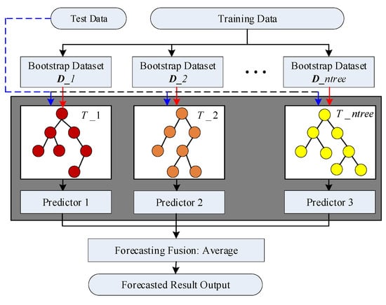
Figure 2. Structural diagram of a random forest.

2.2. Meta-Learning Enhanced RFs Ensemble Methods

Meta-learning, particularly through stacking frameworks, represents a highly effective strategy for enhancing machine learning performance in hierarchical models [32,33]. Specifically, in short-term forecasting, stacking independent forecasts for consecutive future steps generated by base learners provides a powerful mechanism to capture inherent temporal dependencies [34]. The employment of random forests (RF) as base learners within this hierarchical framework enables an effective combination of RFs spatial representation learning capabilities with temporal correlations across short-term forecast horizons [35]. The following sections detail three solution variants developed within this framework.

2.2.1. RF-Meta

Initially, a hierarchical stacking meta-learning structure, termed RF-Meta, is employed for forecasting. This approach trains independent random forest (RF) base learners to generate forecasts for each future step. Subsequently, a separate RF meta-learner at the final layer combines predictions from all base learners corresponding to each specific future time step. The RF-Meta forecasting procedure is summarized in Algorithm A1.

2.2.2. RRF-Meta-FCN

Section 2.2.1 identifies a key limitation: temporal information within the target series is primarily incorporated only at the meta-learning layer, which is insufficient. To address this limitation, a recursive organization of random forest (RF) base learners, termed Recursive RF Base Learners, is proposed. Specifically, the value at the immediate future time step (t + 1) is first estimated using the preceding T known historical inputs. This forecasted value is then combined with the last T−1 known inputs to estimate the subsequent time step (t + 2). The process iterates sequentially, as illustrated in Figure 1, where estimation of the ith future time step (t + i) incorporates i − 1 previously forecasted values. Finally, a Fully Connected Network (FCN) serves as the meta-learner, integrating all outputs from the recursive RF base learner layer to generate simultaneous short-term multi-step forecasts. The detailed implementation of this RRF-Meta-RF approach is provided in Algorithm A2. Accordingly, replacing the final meta-learning RFs with an MIMO FCN results in the RRF-Meta-FCR method.

3. Experimental Results

This section evaluates the short-term forecasting performance of the proposed methods using monthly production data from 2558 oil wells in a specific block of the Daqing Oilfield, with a maximum historical record length of 67 months. The middle depth of the target formation of the aforementioned wells ranges from 1000 to 1200 m, classifying them as medium-porosity and medium-permeability reservoirs. Additionally, the crude oil exhibits the characteristics of high wax content, high freezing point, and high viscosity. For comparison, two established short-term forecasting methods-LSTM and CNN-BiLSTM- are included as benchmarks, as both methods inherently capture short-term temporal information. All evaluated methods adopt standard parameter configurations from the literature: 100 trees, an initial learning rate of 0.01, 128 LSTM neurons, a CNN kernel size of 3, and 32 CNN filters.

Prior to the experiments, the issue of missing data was addressed using a non-local mean embedding technique. This technique operates as follows: for a given missing value or segment $S\in {ℝ}^{L\times 1}$ (where 1 ≤ L ≤ 5 is the length of the missing data segment; if L > 5, this segment of data is discarded), similar non-local target segments $S_t\in {ℝ}^{3L\times 1}$ are identified across the entire dataset, as illustrated in Figure 3. Subsequently, the missing value is imputed by performing a non-local mean embedding, which calculates a weighted average of these similar segments:

$$S={\displaystyle \frac{{\displaystyle \sum _{S_e\in N\left(S_t\right)}{S}_e\left(L+1:2L\right)}}{len\left(N\left(S_t\right)\right)}}$$

(2)

where $N\left(S_t\right)$ represents the set of non-local nearest neighbors for the missing segment S_t, and $len\left(N\left(S_t\right)\right)$ denotes the total number of such neighbors.

Figure 3. Illustration of target segment construction for missing data recovery.

The evaluation indicators are as follows:

$$RMSE=\sqrt{{\displaystyle \frac{1}{N}}{\displaystyle \sum _{i=1}^N{\left(Y_i-{\tilde{Y}}_i\right)}^2}}$$

(3)

$$MAE={\displaystyle \frac{1}{N}}{\displaystyle \sum _{i=1}^N\left|Y_i-{\tilde{Y}}_i\right|}$$

(4)

$$MAPE={\displaystyle \frac{100\%}{N}}{\displaystyle \sum _{i=1}^N\left|\frac{Y_i-{\tilde{Y}}_i}{Y_i}\right|}$$

(5)

$$R^2=1-{\displaystyle \frac{{\displaystyle \sum _{i=1}^N{\left(Y_i-{\tilde{Y}}_i\right)}^2}}{{\displaystyle \sum _{i=1}^N{\left(Y_i-{\overline{Y}}_i\right)}^2}}}$$

(6)

where $Y_i$ represents the known target value, ${\tilde{Y}}_i$ denotes the predicted value, and ${\overline{Y}}_i$ is the mean of target values, and N indicates the number of forecasting samples.

3.1. Experiment 1: 3-Step Short-Term Production Forecasting

The experiment conducts a three-step short-term production forecasting study with two primary objectives: (1) performance comparison with LSTM and CNN-BiLSTM benchmarks; (2) evaluation of input and output length effects on the proposed methods (RF-Meta, RRF-Meta-RF, and RRF-Meta-FCN).

To achieve these objectives, the output length was fixed at three while varying the input sizes (6, 8, 10, and 12 months). The corresponding evaluation results for each input length configuration are shown in Table 1, Table 2, Table 3 and Table 4.

Table 1. Evaluation results comparison under a 6-input-3-output configuration.

6-3	RMSE			MAE			R2			MAPE
	t + 1	t + 2	t + 3	t + 1	t + 2	t + 3	t + 1	t + 2	t + 3	t + 1	t + 2	t + 3
RF-Meta	0.582	0.708	0.784	0.205	0.287	0.350	0.879	0.822	0.781	13.19	18.76	23.54
LSTM	1.043	1.136	1.220	0.618	0.664	0.689	0.613	0.542	0.471	71.91	77.08	82.20
CNN-BiLSTM	0.685	0.790	0.849	0.305	0.369	0.423	0.833	0.778	0.744	27.44	30.82	36.71
RRF-MetaRF	0.591	0.700	0.786	0.219	0.293	0.356	0.876	0.826	0.781	14.29	19.45	24.17
RRF-MetaFCN	0.590	0.693	0.776	0.223	0.282	0.339	0.876	0.829	0.786	14.65	18.78	22.98

Table 2. Evaluation results comparison under an 8-input-3-output configuration.

8-3	RMSE			MAE			R2			MAPE
	t + 1	t + 2	t + 3	t + 1	t + 2	t + 3	t + 1	t + 2	t + 3	t + 1	t + 2	t + 3
RF-Meta	0.570	0.691	0.762	0.205	0.283	0.348	0.884	0.830	0.791	12.69	18.28	22.59
LSTM	0.752	0.822	0.874	0.453	0.465	0.490	0.798	0.758	0.724	24.95	26.58	28.47
CNN-BiLSTM	0.625	0.739	0.811	0.249	0.322	0.372	0.861	0.805	0.736	15.50	21.80	23.32
RRF-MetaRF	0.578	0.679	0.763	0.218	0.286	0.352	0.881	0.835	0.790	13.52	18.60	22.97
RRF-MetaFCN	0.575	0.677	0.758	0.215	0.275	0.337	0.882	0.836	0.793	14.05	18.43	22.25

Table 3. Evaluation results comparison under a 10-input-3-output configuration.

10-3	RMSE			MAE			R2			MAPE
	t + 1	t + 2	t + 3	t + 1	t + 2	t + 3	t + 1	t + 2	t + 3	t + 1	t + 2	t + 3
RF-Meta	0.567	0.692	0.778	0.202	0.285	0.350	0.888	0.833	0.789	11.75	16.56	20.95
LSTM	0.754	0.829	0.915	0.473	0.477	0.519	0.801	0.760	0.708	24.71	24.05	25.49
CNN-BiLSTM	0.738	0.812	0.882	0.317	0.364	0.407	0.811	0.770	0.729	20.80	22.51	24.92
RRF-MetaRF	0.575	0.676	0.772	0.216	0.287	0.351	0.885	0.840	0.793	12.59	16.67	21.13
RRF-MetaFCN	0.571	0.668	0.767	0.207	0.280	0.343	0.887	0.844	0.795	12.49	16.77	21.61

Table 4. Evaluation results comparison under a 12-input-3-output configuration.

12-3	RMSE			MAE			R2			MAPE
	t + 1	t + 2	t + 3	t + 1	t + 2	t + 3	t + 1	t + 2	t + 3	t + 1	t + 2	t + 3
RF-Meta	0.565	0.683	0.769	0.206	0.287	0.352	0.887	0.835	0.789	12.00	17.27	21.21
LSTM	0.798	0.887	0.942	0.495	0.522	0.546	0.774	0.721	0.684	29.70	30.97	29.80
CNN-BiLSTM	0.631	0.741	0.831	0.264	0.330	0.395	0.858	0.805	0.754	15.98	20.60	24.52
RRF-MetaRF	0.575	0.667	0.764	0.221	0.288	0.354	0.883	0.842	0.792	12.92	17.43	21.43
RRF-MetaFCN	0.570	0.650	0.760	0.227	0.276	0.349	0.885	0.850	0.795	12.42	16.56	19.72

Figure 4 presents forecasting results for both 6-input-3-output and 12-input-3-output configurations. The regression performance comparisons are illustrated in Figure 5 and Figure 6, while the comprehensive comparative analysis is shown in the radar charts (Figure 7 and Figure 8).

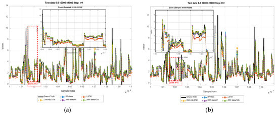
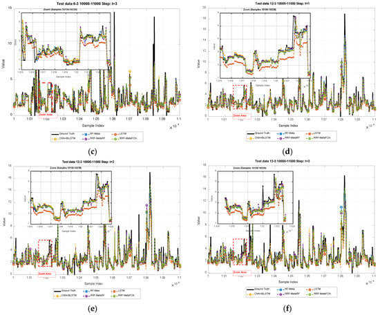
Figure 4. Illustration of short-term forecasting results of: (a–c) 3-steps of 6-input-3-output; (d–f) 3-steps of 12-input-3-output.

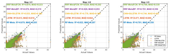
Figure 5. Regression performance comparison for data with a 6-input-3-output configuration.

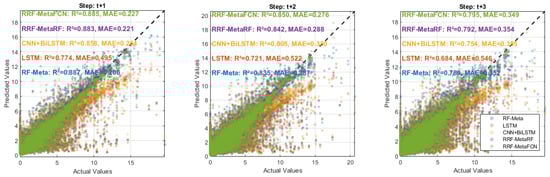
Figure 6. Regression performance comparison for data with a 12-input-3-output configuration.

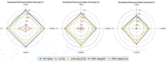
Figure 7. Radar chart for forecasting performance of data with a 6-input-3-output configuration.

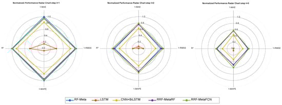
Figure 8. Radar chart for forecasting performance of data with a 12-input-3-output configuration.

3.2. Experiment 2: 6-Step Short-Term Production Forecasting

The experiment extends the forecasting horizon to 6 months (half a year) with a 12-month (one-year) input length. The evaluation results are presented in Figure 9, while Figure 10 displays the forecasting results. Figure 11 and Figure 12 show the regression performance comparison and comprehensive comparative analysis (in radar chart form), respectively.

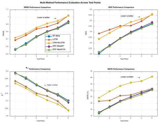
Figure 9. Forecasting result curves of data with a 12-input-6-output configuration.

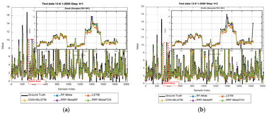
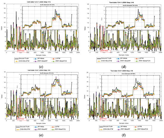
Figure 10. Illustration of short-term forecasting results with 12-input-3-output configuration: (a–f) are results of t + 1 to t + 6.

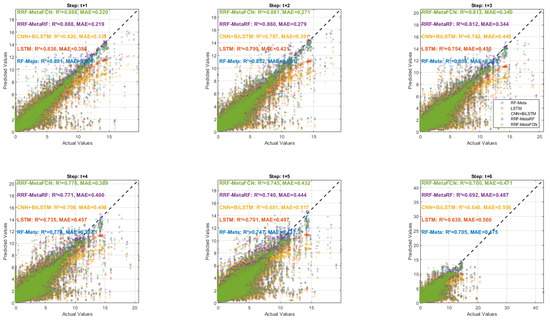
Figure 11. Regression performance comparison for data with a 12-input-6-output configuration.

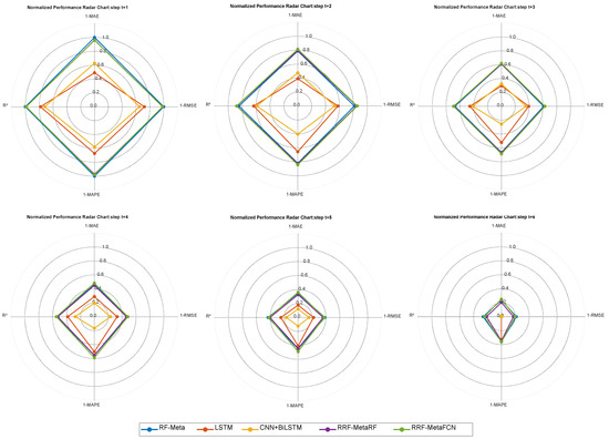
Figure 12. Radar chart for forecasting performance of data with a 12-input-6-output configuration.

In addition to the above results, some of the single forecasting results of data with 12-input-3-output and 12-input-6-output configurations are presented in Figure 13 and Figure 14.

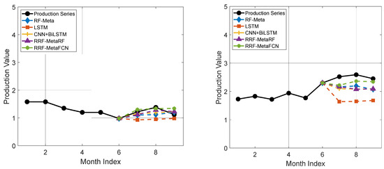
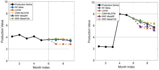
Figure 13. Examples of short-term production forecasting results illustration for data with 12-input-3 output.

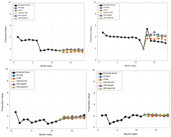
Figure 14. Examples of short-term production forecasting results illustration for data with 12-input-6 output.

3.3. Discussion

The core of this study focuses on employing meta-learning with random forest (RF) as base learners to integrate spatial-temporal information for enhanced short-term production forecasting. Results demonstrate that all three proposed methods significantly outperform both LSTM and CNN-BiLSTM benchmarks. Specifically, Figure 15 quantifies performance gains over CNN-BiLSTM (which performs better than LSTM), while Figure 16 shows improvements against CNN-BiLSTM for 6-output scenarios. The proposed meta-learning RF ensemble framework exhibits robust performance in short-term production forecasting. Among the three variants: (1) RF-Meta achieves optimal near-term forecasts; (2) RRF-Meta-FCN performs best for longer horizons where temporal correlations diminish. This hierarchical recursive architecture effectively captures temporal information through multiple RF base learners. However, RRF-Meta-FCN’s enhanced capability requires significantly higher computational cost than RF-Meta.

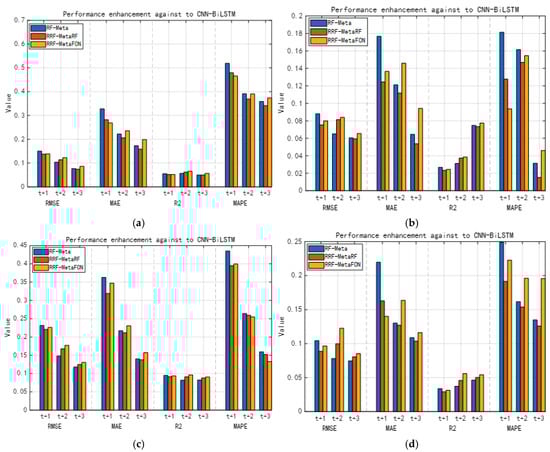
Figure 15. Performance gains of short-term production forecasting of the proposed methods against CNN-BiLSTM: (a) 6-input-3-output; (b) 8-input-3-output; (c) 10-input-3-output; (d) 12-input-3-output.

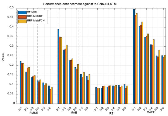
Figure 16. Performance gains of short-term production forecasting of the proposed methods against CNN-BiLSTM for the 12-input-6-output case.

4. Conclusions

This study presents a meta-learning enhanced random forest framework designed to improve temporal correlation modeling in short-term production forecasting. Through extensive experiments on industrial-scale datasets, three novel variants—RF-Meta, RRF-Meta-RF, and RRF-Meta-FCN—show significant performance improvements. Key conclusions can be summarized as:

Short-term sequential deployment of RF through meta-learning (RF-Meta) effectively captures temporal dependencies while maintaining RFs inherent advantages in non-linear representation and robustness. The method achieves > 15% RMSE reduction in 3-step forecasting compared to CNN-BiLSTM (as validated in Figure 15).

RF-Meta demonstrates exceptional performance for immediate horizons (≤6 steps) with single-layer meta-learning. However, its temporal utilization efficiency decreases in prediction horizons that extend beyond six steps due to decaying feature–target correlations.

RRF-Meta-FCN addresses long-horizon limitations through multi-level sequential RF meta-learners, enabling improved temporal information propagation. This enhancement requires substantially greater computational resources compared to RF-Meta.

Overall, the hierarchical meta-RF framework significantly improves temporal correlation utilization in production forecasting. For practical implementation: (1) RF-Meta represents the optimal choice for real-time scenarios requiring <6-step predictions with limited resources; (2) RRF-Meta-FCN provides extended forecasting capability but necessitates high-performance computing infrastructure.

4.1. Limitations

While this study demonstrates the efficacy of the meta-enhanced RF framework, several limitations warrant acknowledgment and present avenues for future research.

(1) The superior long-horizon forecasting of RRF-Meta-FCN is achieved at the cost of high computational complexity, potentially limiting its use in real-time applications with limited resources.

(2) The current study validates the framework on specific industrial datasets, and its generalizability across different production types or geological settings requires further extensive verification.

4.2. Future Work

To address the aforementioned limitations, our future work will enhance the meta-enhanced RF models from the following aspects:

(1) Developing lightweight or distributed versions of the RRF-Meta-FCN model to mitigate its computational demands.

(2) Investigating the explainability of the RRF-Meta-FCN model to enhance the interpretability and acceptability of its forecasts for petroleum engineers.

(3) Evaluating the robustness and transferability of the RRF-Meta-FCN method across different types of oil fields.

References

- Rodriguez, A.X.; Salazar, D.A. Methodology for the prediction of fluid production in the waterflooding process based on multivariate long–short term memory neural networks. J. Pet. Sci. Eng. 2022, 208, 109715. [Google Scholar] [CrossRef]
- Alkhammash, E.H. An optimized gradient boosting model by genetic algorithm for forecasting crude oil production. Energies 2022, 15, 6416. [Google Scholar] [CrossRef]
- de Oliveira Werneck, R.; Prates, R.; Moura, R.; Goncalves, M.M.; Castro, M.; Soriano-Vargas, A.; Júnior, P.R.M.; Hossain, M.M.; Zampieri, M.F.; Ferreira, A.; et al. Data-driven deep-learning forecasting for oil production and pressure. J. Pet. Sci. Eng. 2022, 210, 109937. [Google Scholar] [CrossRef]
- Wang, L.; Wang, S.; Zhang, R.; Wang, C.; Xiong, Y.; Zheng, X.; Li, S.; Jin, K.; Rui, Z. Review of multi-scale and multi-physical simulation technologies for shale and tight gas reservoirs. J. Nat. Gas Sci. Eng. 2017, 37, 560–578. [Google Scholar] [CrossRef]
- Wang, X.; Hu, Y.; Deng, Y. A model of production data analysis for horizontal wells. Pet. Explor. Dev. 2010, 37, 99–103. [Google Scholar] [CrossRef]
- Arps, J.J. Analysis of Decline Curves. Pet. Trans. 1945, 228–247. [Google Scholar] [CrossRef]
- Lee, W.J.; Sidle, R. Gas-Reserves Estimation in Resource Plays. SPE Econ. Manag. 2010, 2, 86–91. [Google Scholar] [CrossRef]
- Ning, Y.; Kazemi, H.; Tahmasebi, P. A comparative machine learning study for time series oil production forecasting: ARIMA, LSTM, and Prophet. Comput. Geosci. 2022, 164, 105126. [Google Scholar] [CrossRef]
- Negash, B.M.; Yaw, A.D. Artificial neural network based production forecasting for a hydrocarbon reservoir under water injection. Pet. Explor. Dev. 2020, 47, 383–392. [Google Scholar] [CrossRef]
- Cheng, H.; Yu, H.; Zeng, P.; Osipov, E.; Li, S.; Vyatkin, V. Automatic Recognition of Sucker-Rod Pumping System Working Conditions Using Dynamometer Cards with Transfer Learning and SVM. Sensors 2020, 20, 5659. [Google Scholar] [CrossRef]
- Dong, Y.; Qiu, L.; Lu, C.; Song, L.; Ding, Z.; Yu, Y.; Chen, G. A data-driven model for predicting initial productivity of offshore directional well based on the physical constrained eXtreme gradient boosting (XGBoost) trees. J. Pet. Sci. Eng. 2022, 211, 110176. [Google Scholar] [CrossRef]
- Lu, C.; Jiang, H.; Yang, J.; Wang, Z.; Zhang, M.; Li, J. Shale oil production prediction and fracturing optimization based on machine learning. J. Pet. Sci. Eng. 2022, 217, 110900. [Google Scholar] [CrossRef]
- Yu, T.K.; Chang, I.C.; Chen, S.D.; Chen, H.L.; Yu, T.Y. Predicting potential soil and groundwater contamination risks from gas stations using three machine learning models (XGBoost, LightGBM, and Random Forest). Process Saf. Environ. Prot. 2025, 199, 107249. [Google Scholar] [CrossRef]
- Sánchez, J.C.M.; Mesa, H.G.A.; Espinosa, A.T.; Castilla, S.R.; Lamont, F.G. Improving Wheat Yield Prediction through Variable Selection Using Support Vector Regression, Random Forest, and Extreme Gradient Boosting. Smart Agric. Technol. 2025, 10, 100791. [Google Scholar] [CrossRef]
- Sabri, A.A.M.; Tomy, S.; Za’in, C. Comparative Machine Learning Analysis for Gold Mineral Prediction Using Random Forest and XGBoost: A Data-Driven Study of the Greater Bendigo Region, Victoria. Geomatica 2025, 77, 100066. [Google Scholar] [CrossRef]
- Chowdhury, S.; Saha, A.K.; Das, D.K. Hydroelectric power potentiality analysis for the future aspect of trends with R2 score estimation by XGBoost and random forest regressor time series models. Procedia Comput. Sci. 2025, 252, 450–456. [Google Scholar] [CrossRef]
- Hamidou, S.T.; Mehdi, A. Enhancing IDS performance through a comparative analysis of Random Forest, XGBoost, and Deep Neural Networks. Mach. Learn. Appl. 2025, 22, 100738. [Google Scholar] [CrossRef]
- Song, X.; Liu, Y.; Xue, L.; Wang, J.; Zhang, J.; Wang, J.; Jiang, L.; Cheng, Z. Time-series well performance prediction based on Long Short-Term Memory (LSTM) neural network model. J. Pet. Sci. Eng. 2020, 186, 106682. [Google Scholar] [CrossRef]
- Kumar, B.; Yadav, N. A novel hybrid model combining βSARMA and LSTM for time series forecasting. Appl. Soft Comput. 2023, 134, 110019. [Google Scholar] [CrossRef]
- Cao, Z.; Song, Q.; Xing, K.; Han, J.; Qie, D. A Novel Multihead Attention-Enhanced Convolutional Neural Network-Long Short-Term Memory Encoder-Decoder for Oil Production Forecasting. SPE J. 2025, 30, 1010–1023. [Google Scholar] [CrossRef]
- Jia, J.; Li, D.; Wang, L.; Fan, Q. Novel Transformer-based deep neural network for the prediction of post-refracturing production from oil wells. Adv. Geo-Energy Res. 2024, 13, 119–131. [Google Scholar] [CrossRef]
- Al-Ali, Z.A.A.H.; Horne, R. Probabilistic Well Production Forecasting in Volve Field Using Temporal Fusion Transformer Deep Learning Models. In Proceedings of the Gas & Oil Technology Showcase and Conference, Dubai, United Arab Emirates, 13–15 March 2023; D031S046R003. [Google Scholar] [CrossRef]
- Zhang, J.; Liu, Y.; Zhang, F.; Li, Y.; Yang, X.; Wang, K.; Ma, Y.; Zhang, N. Integrating petrophysical, hydrofracture, and historical production data with self-attention-based deep learning for shale oil production prediction. SPE J. 2024, 29, 6583–6604. [Google Scholar] [CrossRef]
- Tripathi, B.K.; Kumar, I.; Kumar, S.; Singh, A. Deep Learning–Based Production Forecasting and Data Assimilation in Unconventional Reservoir. SPE J. 2024, 29, 5189–5206. [Google Scholar] [CrossRef]
- Zhang, K.; Wang, Q.; Wang, L.; Zhang, H.; Zhang, L.; Yao, J.; Yang, Y. Fault diagnosis method for sucker rod well with few shots based on meta-transfer learning. J. Pet. Sci. Eng. 2022, 212, 110295. [Google Scholar] [CrossRef]
- Breiman, L. Random forests. Mach. Learn. 2001, 45, 5–32. [Google Scholar] [CrossRef]
- Sukhija, S.; Krishnan, N.C. Supervised heterogeneous feature transfer via random forests. Artif. Intell. 2019, 268, 30–53. [Google Scholar] [CrossRef]
- Tong, S.; Wang, F.; Gao, H.; Zhu, W. A machine learning-based method for analyzing factors influencing production capacity and production forecasting in fractured tight oil reservoirs. Int. J. Hydrogen Energy 2024, 70, 136–145. [Google Scholar] [CrossRef]
- Breiman, L.; Friedman, J.; Olshen, R.A.; Stone, C.J. Introduction to Tree Classification. In Classification and Regression Trees; Chapman and Hall/CRC: New York, NY, USA, 1984. [Google Scholar] [CrossRef]
- Efron, B. Bootstrap Methods: Another Look at the Jackknife. Ann. Stat. 1979, 7, 1–26. [Google Scholar] [CrossRef]
- Altman, N.; Krzywinski, M. Ensemble methods: Bagging and random forests. Nat. Methods 2017, 14, 933–934. [Google Scholar] [CrossRef]
- Wang, M.; Su, X.; Song, H.; Wang, Y.; Yang, X. Enhancing predictive maintenance strategies for oil and gas equipment through ensemble learning modeling. J. Pet. Explor. Prod. Technol. 2025, 15, 46. [Google Scholar] [CrossRef]
- Azadivash, A.; Soleymani, H.; Seifirad, A.; Sandani, A.; Yahyaee, F.; Kadkhodaie, A. Robust fracture intensity estimation from petrophysical logs and mud loss data: A multi-level ensemble modeling approach. J. Pet. Explor. Prod. Technol. 2024, 14, 1859–1878. [Google Scholar] [CrossRef]
- Hochreiter, S.; Schmidhuber, J. Long short-term memory. Neural Comput. 1997, 9, 1735–1780. [Google Scholar] [CrossRef]
- Smyth, P.; Wolpert, D. Linearly combining density estimators via stacking. Mach. Learn. 1999, 36, 59–83. [Google Scholar] [CrossRef]
Disclaimer/Publisher’s Note: The statements, opinions and data contained in all publications are solely those of the individual author(s) and contributor(s) and not of MDPI and/or the editor(s). MDPI and/or the editor(s) disclaim responsibility for any injury to people or property resulting from any ideas, methods, instructions or products referred to in the content. |
© 2025 by the authors. Licensee MDPI, Basel, Switzerland. This article is an open access article distributed under the terms and conditions of the Creative Commons Attribution (CC BY) license (https://creativecommons.org/licenses/by/4.0/).