Low-Carbon Demand Response Strategy for Park-Level Integrated Energy Systems Based on Typical Electricity–Carbon Coupling Scenarios

Abstract

This paper addresses the low-carbon operation of integrated energy systems (PIESs) by proposing a carbon-aware demand response strategy with synergistic participation from consumers and energy storage. Initially, two typical scenarios—“electricity–carbon peak alignment” and “electricity–carbon peak misalignment”—are generated based on uncertainties in renewable generation and load profiles. These scenarios aim to characterise the coupling relationship between electricity and carbon emissions, providing a contextual basis for guiding responsive behaviours of consumers and storage systems. Subsequently, a carbon emission flow model incorporating energy conversion and storage is developed to quantify the carbon emission impacts of both consumers and energy storage units. Furthermore, a carbon-aware demand response strategy is formulated using dynamic carbon signals, coupled with an assessment model for carbon reduction benefits. Experimental validation across both scenarios demonstrates the efficacy of the proposed strategy in promoting low-carbon PIES operation. Compared to traditional electricity demand response, the proposed low-carbon demand response strategy enhances carbon emission reduction by 21.5% under the “electricity–carbon peak alignment” scenario, and this reduction even doubles under the “electricity–carbon peak misalignment” scenario. Additionally, the integration of energy storage for response increases the park’s average carbon reduction by 15%. This demonstrates that the strategy proposed in this paper significantly improves the park’s capability for carbon emission reduction.

1. Introduction

A park-level integrated energy system (PIES) is an energy supply framework within a specific geographical boundary that, through an integrated planning and intelligent management platform, achieves the synergistic production, efficient conversion, optimised storage, and rational consumption of various energy forms such as electricity, heat, cooling, and gas. Its core characteristics are manifested as “horizontal multi-energy complementarity” and “vertical source–grid–load–storage coordination,” which can effectively enhance the park’s energy self-sufficiency rate and comprehensive energy utilisation efficiency. The PIES represents a typical application of integrated energy systems at the regional level. It places a greater emphasis on the integrated utilisation of distributed new energy generation equipment, demand-side flexibility resources, and low-carbon technologies. The PIES can provide users with more economical, efficient, and environmentally friendly integrated energy services. Consequently, achieving the low-carbon optimal operation of PIESs has become a current research hotspot [1,2,3].

Existing research has proposed various carbon reduction methods for PIESs. Some scholars have focused on reducing direct carbon emissions from the power supply side, employing technologies such as Carbon Capture and Storage (CCS) and Power-to-Gas (P2G) to promote the low-carbon transition of energy equipment within the system. For instance, references [4,5] introduced P2G and CCS equipment into an integrated energy system dominated by Combined Heat and Power (CHP) units, proposing an optimal scheduling model aimed at minimising operating costs. Through the optimal scheduling of the integrated energy system, they addressed the issues of high costs for externally sourced carbon for P2G and high carbon emissions from CHP. On the load side, employing demand response (DR) to guide users in adjusting their energy consumption patterns is also a crucial approach for optimising the low-carbon operation of PIESs and alleviating the conflict between energy supply and demand [6]. For example, reference [7] established a tiered compensation price incentive mechanism and considered the participation of smart parking lots and hydrogen fuel vehicles in demand response. Reference [8] conducted refined modelling of conventional demand response, analysed the coupling characteristics of cooling, heating, and electrical loads, and established an optimal scheduling model for a PIES with supply–demand-side interaction, aiming to minimise operating costs. Reference [9] proposed a low-carbon optimal scheduling method for a hydrogen-integrated energy system, considering the combination of green certificates, carbon trading, and demand response.

The aforementioned literature primarily investigates demand response from economic and technical perspectives. Against the backdrop of the “dual carbon” goals, exploring the carbon reduction potential of demand-side resources with a low-carbon objective has gradually become a new research hotspot. Some scholars have calculated dynamic carbon emission factors using the carbon emission flow analysis method for power systems, using this as a guiding signal to propose a low-carbon demand response (LCDR) mechanism [10]. Low-carbon demand response is a carbon reduction mechanism that utilises dynamic carbon emission factors as guiding signals. It enables the load side to gain real-time awareness of the variations in the carbon intensity of electricity consumption, thereby steering consumers toward low-carbon electricity usage behaviours to achieve system-wide carbon reduction. Reference [10] introduced this mechanism into integrated energy systems, shifting the research focus from an “electricity perspective” to a “carbon perspective.” For example, reference [11], focusing on an integrated energy system with coal-to-hydrogen and carbon capture power plants, introduced an LCDR mechanism and established a low-carbon economic dispatch model for the system with the objective of minimising operating costs. The study in reference [12] considered both the source and load sides, incorporating a carbon-trading mechanism on the supply side and considering carbon emission issues on the user side. It utilised incentive-based LCDR to guide low-carbon dispatch on the supply side and proposed an optimal scheduling model for an integrated energy system that considers LCDR and a supply–demand master–slave game. Furthermore, a few scholars have paid attention to the role of energy storage in reducing the carbon emissions of PIESs. Reference [13] proposed an extended carbon emission flow model for energy storage devices. Based on this model, a “carbon tax” demand response model was used for a bi-level game between the park and users internally, while a Nash bargaining model was employed to simulate the game behaviour of various entities participating in the carbon-trading market among multiple parks. This led to the establishment of an optimal scheduling model for a park-level integrated energy system based on a dual game on both the supply and demand sides.

From the analysis of the current research status, it is evident that most carbon emission reduction studies for park-level integrated energy systems (PIESs) focus on the source and load sides, with low-carbon demand response gaining increasing attention. However, existing work still lacks an effective quantification of the relationship between changes in user electricity consumption behaviour and the corresponding carbon emissions. This makes it difficult for users to intuitively perceive the actual contribution of their actions to carbon reduction, thereby limiting their motivation to participate in demand response. Meanwhile, in low-carbon demand response, users adjust their electricity consumption timing to align with the system’s carbon regulation, while energy storage, as a flexible “virtual user,” can regulate the spatiotemporal distribution of carbon flow by altering its charging and discharging behaviour. The synergistic interaction between users and energy storage, based on a unified carbon signal, can jointly enhance the low-carbon level of the PIES. Therefore, an in-depth study of the synergistic relationship and regulatory potential of “users plus energy storage” participation in low-carbon demand response is of great significance for improving the carbon reduction capabilities of PIESs. Crucially, within a PIES, “electricity” serves as the carrier of energy flow, and its supply–demand status directly determines the system’s operation. In contrast, “carbon,” as a byproduct of energy conversion, reflects the environmental impact of energy consumption. The superimposed dual uncertainties of renewable energy output from wind and solar, along with load fluctuations, cause the electricity–carbon coupling relationship to change dynamically [14,15], significantly increasing the complexity of low-carbon optimal operation. Consequently, the core of PIESs’ low-carbon operation research lies in seeking the optimal dispatch scheme for the system amidst the dynamically varying electricity–carbon correlation. Therefore, it is essential to deeply elucidate the intrinsic dynamic patterns of electricity–carbon coupling, based on an analysis of source and load uncertainties, thereby providing a benchmark framework for the formulation and validation of low-carbon demand response strategies.

In summary, existing research has not yet effectively quantified the specific contribution of these behaviours to carbon emission reduction, nor has it fully revealed the impact of the electricity–carbon coupling relationship on the synergistic response patterns of users and energy storage under source–load uncertainty. To address these issues, this paper treats energy storage as a “virtual user” and, based on an analysis of the electricity–carbon coupling relationship, investigates a low-carbon demand response strategy involving the coordinated participation of “users plus energy storage” to deeply explore their synergistic potential for carbon reduction by responding to dynamic carbon signals. Firstly, based on the historical operational data of the park, scene generation and reduction techniques will be employed to extract two typical scenarios—“electricity–carbon peak alignment” and “electricity–carbon peak misalignment”—to reveal the dynamic characteristics of electricity–carbon coupling under different source–load conditions. Secondly, a PIES low-carbon operational framework with source–load–storage coordination will be constructed. A carbon emission flow model will be introduced to characterise the carbon flow properties of various types of equipment, and dynamic updates of user-side carbon emission intensity will be achieved through a comprehensive carbon flow balance across all links. On this basis, an incentive signal guided by a dynamic carbon factor will be introduced, and a coordinated low-carbon demand response strategy for “user plus energy storage” guided by this carbon signal will be proposed. Finally, the effectiveness of the proposed strategy in enhancing the system’s low-carbon operational performance will be verified based on the two aforementioned typical electricity–carbon scenarios.

2. Typical Scenarios of Electricity–Carbon Coupling in PIES

The intermittency and volatility of renewable energy sources such as wind and solar power combined with the randomness and diversity of load demand, along with their interactions, constitute key drivers for dynamic changes in the electricity–carbon coupling relationship within PIESs. This section constructs multiple sets of time-series scenarios for source–load combinations. Through analysing the correlation between carbon flow and operational states under various renewable energy output and load level configurations, we define typical electricity–carbon coupling scenarios for PIESs. This establishes the foundation for further investigation into the effectiveness of low-carbon demand response strategies.

2.1. Optimal Scenario Generation Considering Spatiotemporal Correlations of Wind–Solar–Load Characteristics

Given the pronounced stochasticity of wind–solar–load distributions, nonparametric kernel density estimation (KDE) effectively circumvents parametric estimation biases and provides superior alignment with empirical distributions. Consequently, this paper adopts KDE to determine the marginal distributions of wind–solar–load variables. The kernel density estimator is defined as follows [16]:

$${\widehat{f}}_h(x)={\displaystyle \frac{1}{nh}}{\displaystyle \sum _{i=1}^{n}K(\frac{x-X_i}{h})}$$

(1)

where ${\widehat{f}}_h(x)$ denotes the density function of the sample points $X_1,X_2,\cdots ,X_n$ at any given point x; h is the bandwidth; and $K\left(\cdot \right)$ represents the kernel function.

To capture the temporal correlation of renewable generation and load, the marginal distribution of each variable is first modelled based on historical data. Subsequently, the inherent dependencies among wind power, photovoltaic output, and load demand across consecutive time intervals—commonly observed in practice—are further considered. These dependencies are characterised as a time-evolving stochastic process, represented by a time-dependent random vector $\mathit{P}=(P_1,P_2,...,P_r{)}^{\mathrm{T}}$, where t denotes the prediction horizon. A multivariate normal distribution is introduced by defining $\mathit{P}\sim N({\mu }_0,\Sigma )$, where the expectation ${\mu }_0$ is a t-dimensional zero vector and $\Sigma$ is the covariance matrix structured as

$$\sum =\left[\begin{array}{cccc}{\sigma }_{1,1}& {\sigma }_{1,2}& \dots & {\sigma }_{1,t}\\ {\sigma }_{2,1}& {\sigma }_{2,2}& \dots & {\sigma }_{2,t}\\ ⋮& ⋮& \ddots & ⋮\\ {\sigma }_{t,1}& {\sigma }_{t,2}& \dots & {\sigma }_{t,t}\end{array}\right]$$

(2)

where ${\sigma }_{i,j}=\mathrm{cov}\left(P_i,P_j\right)$ and $i,j=1,2,\cdots ,24$ represent the covariances between variables $P_i$ and $P_j$ across different time periods.

According to the definition of covariance, all main diagonal elements of the covariance matrix $\Sigma$ are unity. Thus, the random vector Z is uniquely determined by $\Sigma$, implying that the temporal dependence of the joint distribution can be fully characterised by the covariance matrix $\Sigma$. An exponential function approach is employed to compute the covariance ${\sigma }_{i,j}$ via Equation (3), where the range parameter ω quantifies the degree of variable correlation. To identify the optimal range parameter ω, a parametric metric $I_s$ is introduced to measure the discrepancy between the probability density function (PDF) of samples drawn from the multivariate normal distribution and historical data. An objective function is subsequently formulated by minimising $I_s$:

$${\sigma }_{i,j}=\mathrm{cov}(P_i,P_j)=\exp (-{\displaystyle \frac{|i-j|}{\epsilon }}),i,j\in (0,T)$$

(3)

$$\min I_{\epsilon }={\displaystyle \frac{1}{M}}\sum _{s\in S}|p_{\mathrm{pdf}}(s)-p_{\mathrm{pdf}}^{\prime }(s)|$$

(4)

where $\epsilon$ denotes the dynamic correlation strength of variables across different time sequences; M represents the pre-sampling scale; S indicates the set of sampling points s within the PDF interval at different time sequences; and $P_{\mathrm{p}\mathrm{d}\mathrm{f}}^{\prime }\left(s\right)$ and $P_{pdf}\left(s\right)$ refer to the probability density curves of historical data and generated scenarios, respectively.

To characterise the spatial correlation among renewable generation and load, a multivariate joint Copula distribution function is employed to construct their joint probability distribution model [17]. Given the strong dependencies among renewable generation and load variables, this study adopts a C-vine (canonical vine) structure based on conditional Copula theory for modelling. Specifically, the high-dimensional joint Copula is decomposed into a product of multiple bivariate Copula functions, and the final multivariate joint Copula distribution is obtained through parameter estimation. Subsequently, the inverse transform sampling method is applied to sample the established joint Copula distribution of renewable generation and load, thereby generating clustered output scenarios for different time periods. The joint probability distribution expression for the C-vine structure is as follows:

$$\begin{array}{l}{f}_{\mathrm{C}}(x_1,\cdots ,x_n)={\displaystyle \prod _{k=1}^n{f}_k}(x_k).{\displaystyle \prod _{j=1}^{n-1}{\displaystyle \prod _{i=1}^{n-j}{c}_{j,j+1|1,\cdots ,j-1}}}\\ \left[F(x_j|x_1,\cdots ,x_{j-1}),F(x_{j+1}|x_1,\cdots ,x_{j-1})\right]\end{array}$$

(5)

where $c_{j,j+1\mid l,\cdots ,j-1}\hspace{0.17em}(\cdot )$ denotes the Copula probability density function formed by variables $x_j$ and $x_{j+i}$ under the condition of known $x_1,x_2,\cdots ,x_{j-1}$, and $F(x_j\mid x_1,\cdots ,x_{j-1})$ represents the distribution function of variable $x_j$ under the condition of known $x_1,x_2,\cdots ,x_{j-1}$.

The conditional distribution possesses the following properties:

$$F(x|\nu )={\displaystyle \frac{\partial C[F(x|{\nu }_{-j}),F({\nu }_j|{\nu }_{-j})]}{\partial F({\nu }_j|{\nu }_{-j})}}$$

(6)

where $v_j$ denotes the $j$ variable in vector $\nu$ and $v_{-j}$ represents the vector formed by removing $v_j$ from vector $\nu$.

Although vine structures can capture correlations among multivariate variables, they still fall short of comprehensively describing interdependencies between every variable pair. Therefore, this study introduces mixed Copula functions during the selection of optimal pairs of Copula components. The methodology primarily incorporates five commonly used Copula types: Gaussian Copula, t-Copula, Gumbel Copula, Clayton Copula, and Frank Copula. The constructed mixed Copula formulation is expressed as

$$C(u,v)={\lambda }_1{C}_1(u_1,v_1;{\theta }_1)+{\lambda }_2{C}_2(u_2,v_2;{\theta }_2)+\dots +{\lambda }_n{C}_n(u_n,v_n;{\theta }_n)$$

(7)

where $u,v$ denotes the marginal distribution of random variables; ${\lambda }_1,{\lambda }_2,\cdots ,{\lambda }_n\in [0,1]$ represents the weight parameter, which satisfies the constraint ${\lambda }_1+{\lambda }_2+,\cdots ,+{\lambda }_n=1$ and quantifies the proportional contribution of each Copula function; and ${\theta }_1,{\theta }_2,\cdots ,{\theta }_n$ is the dependence coefficient, indicating the relative weight of an individual Copula and characterising the correlation between variables.

Based on the spatiotemporal characterisation of wind, solar, and load described above, this study utilises actual data for wind turbine output, photovoltaic (PV) output, and load from a representative industrial park in Pudong New Area, Shanghai, China, for the entire year of 2022. By further incorporating Monte Carlo sampling, 5000 output scenarios that account for the correlation between wind and solar power are generated, as shown in Figure A1, Appendix A.

2.2. Definition and Analysis of Typical Scenarios for Electricity–Carbon Coupling in PIES

Based on the renewable generation and load output scenarios obtained in Section 2.1, the K-means clustering algorithm is further employed for scenario reduction, ultimately yielding five typical scenarios as illustrated in Figure 1. The curves of renewable generation and load across these scenarios reveal significant temporal complementarity or synchronisation. In Scenario 1, the photovoltaic output peaks at midday, coinciding with the load peak, whereas in Scenario 3, wind power generation is higher at night, while load demand remains at a trough.

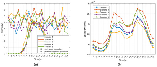
Figure 1. Wind–solar power output and load curves in typical scenarios: (a) renewable power output curves; (b) load curves.

Given that differences in source–load matching relationships directly influence the system’s carbon emission characteristics, dynamic carbon emission factors [13,18,19,20] are introduced to further characterise the carbon intensity of the aforementioned typical scenarios, as shown in Figure 2. Dynamic carbon emission factors reflect the variation in carbon emissions per unit of electricity consumption, which is highly correlated with renewable energy output: higher renewable generation reduces reliance on traditional high-carbon units, thereby lowering carbon emissions. By comparing the renewable output curves and carbon intensity curves across typical scenarios in Figure 2, it is observed that in Scenarios 1 and 4, load peaks largely coincide with carbon emission peaks, whereas in Scenarios 2 and 5, carbon emissions remain low during load peak periods due to sufficient renewable energy output. This occurs because the PIES features a high and growing share of the renewable energy capacity, while high-carbon units are gradually phased out. Consequently, carbon emission peaks no longer strictly align with load peaks but are jointly influenced by both load demand and renewable generation. To intuitively reveal the relationship between electricity load and carbon intensity as renewable output varies in PIESs, and to decouple the interactions among renewable generation, load demand, and carbon emissions, the typical scenarios in Figure 2 are further classified in Figure 3, leading to the definition of the following two typical scenarios for electricity–carbon coupling in PIESs.

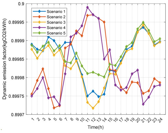
Figure 2. Dynamic carbon emission factor curves in typical scenarios.

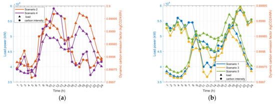
Figure 3. Typical scenarios of electricity–carbon coupling in PIES: (a) electricity–carbon peak alignment scenario; (b) electricity–carbon peak misalignment scenario.

Scenario 1: Electricity–carbon peak alignment. As shown in Figure 3a, this scenario arises when renewable energy output falls within its minimum range during load peak hours due to meteorological conditions (e.g., windless cloudy days and windy nights), while reaching its maximum range during load troughs. During morning and evening load peaks, renewable generation decreases, necessitating increased output from thermal and CHP units to meet electricity demand, thereby elevating carbon intensity to daily peak levels. Conversely, during load troughs, lower demand coincides with higher renewable output, minimising the operation of high-carbon units such as thermal and CHP plants, resulting in the lowest carbon intensity range. The alignment between load curves and dynamic carbon emission factor curves indicates that this scenario resembles traditional systems dominated by thermal and CHP units, where load peaks synchronise with carbon emission peaks. Thus, this study defines it as the “electricity–carbon peak alignment” scenario.

Scenario 2: Electricity–carbon peak misalignment. As illustrated in Figure 3b, this scenario typically occurs during sunny/windy daytime periods and windless nights. During midday and afternoon hours, the increased share of renewable energy (e.g., solar and wind) in the PIES’s power supply significantly reduces reliance on high-carbon units, driving carbon intensity to its lowest levels. Conversely, during evening hours, particularly the evening load peak, diminished renewable output necessitates supplementary power from high-carbon units to meet demand, resulting in peak carbon intensity. The comparative analysis of carbon intensity and load curves reveals a pronounced temporal decoupling: peak electricity demand coincides with troughs in carbon emission intensity. This study defines such patterns as the “electricity–carbon peak misalignment” scenario.

Given that the operational boundaries and evolutionary limits of the coupling relationship between electricity load and dynamic carbon emission factors in PIESs lie between the two typical scenarios of “electricity–carbon peak alignment” and “electricity–carbon peak misalignment”, this study adopts these scenarios as benchmark frameworks to further investigate low-carbon demand response strategies and validate the effectiveness of the proposed approaches.

3. A Low-Carbon Operational Framework for PIES Based on Source–Load–Storage Coordinated Carbon Reduction

The topological structure of the low-carbon PIES studied in this paper is shown in Figure 4. The electricity supply equipment includes wind turbines, photovoltaic (PV) generation units, Combined Heat and Power (CHP) units, and the main grid. The heat supply equipment consists of the CHP unit, a gas boiler, and an electric boiler. Figure 5 illustrates the source–load–storage coordinated carbon reduction framework for the PIES. On the source side, the coupled operation mechanism of Carbon Capture and Storage (CCS) and Power-to-Gas (P2G) directly reduces the carbon emissions of the PIES and enhances the accommodation level of renewable energy. On the load and storage sides, a low-carbon demand response strategy is utilised to indirectly reduce carbon emissions.

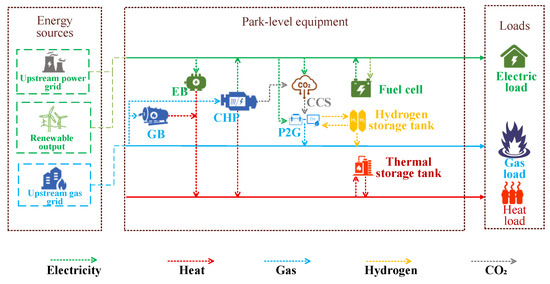
Figure 4. Topology structure of PIES.

Figure 5. The framework source–load–storage coordinated carbon reduction of PIES.

As shown on the left side of Figure 5, although the coupled operation of CCS-P2G can effectively reduce carbon emissions on the source side, the high energy consumption characteristics of CCS and P2G equipment can exacerbate the energy supply–demand conflict within the park during peak load periods. This increases the output of high-carbon-emitting units, while the system lacks surplus electricity for CO₂ capture by CCS, leading to an overall increase in system carbon emissions and insufficient system flexibility to cope with the randomness of renewable energy generation. Consequently, deploying energy storage equipment is considered to alleviate the park’s energy supply–demand pressure and enhance the flexibility of system operation. As depicted on the right side of Figure 5, this paper introduces low-carbon demand response [10] into the PIES. It utilises a dynamic carbon emission factor to characterise the system’s carbon emission intensity [13,18,19,20] and employs it as a guiding signal for low-carbon demand response. Under the low-carbon demand response framework, users within the PIES, guided by the dynamic carbon emission factor, tend to reduce or shift their electricity consumption from peak carbon emission periods to other times and increase consumption during low carbon emission periods to reduce their carbon footprint. Simultaneously, the energy storage system can participate in low-carbon demand response as a virtual user, responding to the carbon signal through a “low-carbon charge, high-carbon discharge” strategy. This means charging during low-carbon periods and discharging during high-carbon periods, which not only generates economic benefits from the carbon market but also effectively lowers the PIES’s carbon emission level. Thus, a closed-loop incentive for carbon reduction is formed on the load and storage sides, supporting the paradigm shift of the PIES from “carbon follows electricity” to “electricity optimised for carbon.”

4. Low-Carbon Demand Response Strategy and Benefit Quantification Model for PIES

In this study, the core of constructing a low-carbon demand response strategy lies in accurately accounting for carbon emissions from user electricity consumption and energy storage charging/discharging behaviours. To achieve this, dynamic carbon emission factors are introduced into the PIES framework. Dynamic carbon emission factors are quantitative indicators that reflect in real time the carbon intensity per unit of electricity consumption at grid nodes or end-user terminals. Their essence involves coupling power flow analysis with carbon emission flow modelling to trace the spatial distribution and temporal evolution of carbon emissions from generation sources through the grid topology [13,18,19,20]. Based on this, this section first presents a carbon emission flow model for the PIES, including the following: (1) a dynamic carbon emission factor model grounded in carbon emission flow theory to quantify indirect carbon emissions from users; (2) an extended carbon emission flow model for energy conversion devices and storage equipment, incorporating their energy use and emission characteristics to capture carbon emissions from diverse internal energy assets. Using this framework, a low-carbon demand response strategy is developed, leveraging dynamic carbon emission factors as carbon signals and enabling synergistic participation from both users and energy storage systems.

4.1. Carbon Emission Flow Model for PIES

4.1.1. Dynamic Carbon Emission Factor Model for PIES

The dynamic carbon emission factor is grounded in carbon emission flow theory. Due to space constraints, the calculation formulas for carbon flow and the node carbon intensity expressions for the electricity, gas, and heating networks in the PIES are provided in Appendix B, with detailed derivations referenced from [20] and omitted here. To characterise the carbon emissions from user-side electricity consumption, node carbon potential is further computed based on node carbon intensity, reflecting the spatial distribution of carbon emission intensity accompanying electricity transmission from generation to end-users. The dynamic carbon emission factor for the PIES is calculated at electricity consumption nodes, derived as a weighted average of nodal carbon potentials. Its core lies in establishing a quantitative link between network carbon flows and user electricity-related emissions through carbon potential, as expressed in the following formula:

$${\epsilon }_t={\displaystyle \frac{{\displaystyle \sum _{i=1}^N{P}_{L,i,t}\times e_{i,t}}}{{\displaystyle \sum _{i=1}^N{P}_{L,i,t}}}}$$

(8)

where ${\epsilon }_t$ is the dynamic carbon emission factor of PIES at time $t$; $e_{i,t}$ represents the carbon potential at node $i$ at time $t$; $P_{L,i,t}$ indicates the load quantity at node $i$ at time $t$; and $N$ denotes the set of nodes within the coverage range of PIESs.

Based on the dynamically calculated carbon emission factors derived from the above methodology, the carbon emissions generated by users within the PIES during a dispatch cycle can be computed using the following formula:

$$E_i={\displaystyle \sum _t^D{\epsilon }_t{P}_{L,i,t}}$$

(9)

where $E_i$ represents the carbon emissions generated by user $i$ during a dispatch cycle and D denotes the duration of the dispatch cycle.

4.1.2. Carbon Emission Flow Model of Energy Conversion Equipment

According to references [13,21], energy conversion devices within PIESs—such as gas boilers and electric boilers—that transform one form of energy into another single form of energy are classified as single-input single-output (SISO) devices. The carbon emissions embedded in the input energy must be conserved in the output emissions. The carbon emission flow model for such equipment is expressed as follows:

$$Q_t^{\mathrm{out}}={\displaystyle \frac{Q_t^{\mathrm{in}}}{\eta }}$$

(10)

where $Q_t^{\mathrm{in}}$ and $Q_t^{\mathrm{out}}$ denote the carbon emission intensity of the input and output, respectively, of an energy coupling device at time $t$, and $\eta$ represents the efficiency of said energy conversion equipment.

Single-input multi-output (SIMO) devices refer to equipment within PIESs that converts one form of energy into two or more forms of energy, such as Combined Heat and Power (CHP) units. The carbon emissions associated with their inputs and outputs must remain conserved, meaning the carbon emissions generated by the CHP unit’s consumption of natural gas should equal the sum of the carbon emissions from its electricity and heat output.

$$\left\{\begin{array}{l}{Q}_t^{\mathrm{out},\mathrm{e}}={\displaystyle \frac{Q_t^{\mathrm{in},\mathrm{g}}}{2{\eta }_{\mathrm{e}}}}\\ Q_t^{\mathrm{out},\mathrm{h}}={\displaystyle \frac{Q_t^{\mathrm{in},\mathrm{g}}}{2{\eta }_{\mathrm{h}}}}\end{array}\right.$$

(11)

where $Q_t^{\mathrm{in},\mathrm{g}}$ represents the carbon emission intensity resulting from the input gas of a CHP unit at time $t$; $Q_t^{\mathrm{out},\mathrm{e}}$ denotes the carbon emission intensities associated with electricity and heat generation by the CHP unit at time $t$, respectively; and ${\eta }_{\mathrm{e}}$ indicates the power generation efficiency and heat production efficiency of said CHP unit.

After retrofitting the CHP unit with carbon capture equipment, a portion of its original electrical output will be allocated to carbon capture and separation processes, resulting in changes to its net power output. The retrofitted CHP unit essentially trades energy consumption for lower carbon emissions. By treating the CCS (Carbon Capture and Storage) and CHP systems as an integrated unit, the carbon emission intensities at both the power generation and supply sides continue to satisfy the conservation principle of carbon emissions across input and output ports:

$$Q_t^{\mathrm{in},\mathrm{g}}{P}_t^{\mathrm{in},\mathrm{g}}=Q_t^{\mathrm{out},\mathrm{e}}(P_t^{\mathrm{out},\mathrm{e}}-P_t^{\mathrm{CCS}})+Q_t^{\mathrm{out},\mathrm{h}}{P}_t^{\mathrm{out},\mathrm{h}}$$

(12)

where $P_t^{\mathrm{in},\mathrm{g}}$ represents the power input from natural gas to the CHP unit at time $t$; $P_t^{\mathrm{out},\mathrm{e}}$ and $P_t^{\mathrm{out},\mathrm{h}}$ denote the electrical power output and thermal power output of the CHP unit at time $t$, respectively; and $P_t^{\mathrm{CCS}}$ indicates the operational energy consumption of the CCS system at time $t$.

4.1.3. Carbon Emission Flow Model of Energy Storage Devices

As a key flexibility resource in PIESs, energy storage devices can actively respond to carbon signals and participate in low-carbon system regulation through their bidirectional charging and discharging capabilities. During charging, energy storage functions similarly to an electricity consumer, absorbing power from the system and temporarily storing the associated carbon emissions. During discharging, it acts as a special power source, outputting electricity and releasing the stored carbon emissions. Consequently, the carbon emission intensity of energy storage discharge is not a fixed value but depends on the carbon content of the charged electricity, making its emissions inherently dynamic and correlated with the charging/discharging power and state of charge (SOC). To quantify the carbon attributes of energy storage from a carbon perspective, this paper introduces the “carbon loading rate” (CLR) metric, inspired by the concept of SOC. Based on carbon emission flow theory, CLR labels the carbon tags of power flowing into and out of energy storage [13,18,19,20], thereby revealing the characteristics of carbon flow storage and release during energy time-shifting. This further enhances its capability as a virtual user participating in low-carbon demand response. CLR represents the ratio of absorbed carbon emissions to stored electricity in energy storage, i.e., how much carbon emission is associated with each kilowatt-hour of electricity stored. The specific calculation is as follows:

During charging, an energy storage system absorbs electrical energy while simultaneously storing the associated potential carbon emissions. The amount of stored carbon emissions is determined by the charging/discharging power and the carbon emission intensity at the node, calculated as follows:

$$M_t^{\mathrm{cha}}=P_t^{\mathrm{cha}}{Q}_t^{\mathrm{cha}}\Delta t$$

(13)

where $\Delta t$ represents the unit time duration; $M_t^{\mathrm{cha}}$ denotes the carbon emissions stored by the energy storage system during charging; $P_t^{\mathrm{cha}}$ indicates the charging power of the energy storage system; and $Q_t^{\mathrm{cha}}$ corresponds to the carbon emission intensity during the charging process.

During discharge, the energy storage system supplies electrical power to the grid while simultaneously releasing the stored carbon emissions. The carbon emissions attributable to the storage system in this mode are determined by its discharge power and the carbon loading rate (CLR), with the specific calculation method as follows:

$$M_t^{\mathrm{dis}}=P_t^{\mathrm{dis}}{Q}_t^{\mathrm{dis}}\Delta t={\displaystyle \frac{P_t^{\mathrm{dis}}}{{\eta }_{\mathrm{dis}}}}{Q}_{t-1}^{\mathrm{CLR}}\Delta t$$

(14)

where $M_t^{\mathrm{dis}}$ represents the carbon emissions during energy storage discharge; $P_t^{\mathrm{dis}}$ denotes the discharge power of the energy storage system; $Q_t^{\mathrm{dis}}$ indicates the carbon emission intensity during discharge; ${\eta }_{\mathrm{dis}}$ corresponds to the discharge efficiency of the energy storage system; and $Q_{t-1}^{\mathrm{CLR}}$ signifies the carbon loading rate (CLR) from the previous time step.

Based on the preceding analysis, the carbon loading rate (CLR) of an energy storage system at a given moment is determined by its CLR from the previous time step, the current charging/discharging power, and the influence of energy losses during the charging/discharging processes. Consequently, the CLR of the energy storage system at time t is expressed as follows:

$$Q_t^{\mathrm{CLR}}={\displaystyle \frac{Q_{t-1}^{\mathrm{CLR}}{E}_{t-1}^{\mathrm{SOC}}{E}_{es}+M_t^{\mathrm{cha}}-M_t^{\mathrm{dis}}}{E_t^{\mathrm{SOC}}{E}_{es}}}$$

(15)

where $E_t^{\mathrm{SOC}}$ represents the state of charge (SOC) of the energy storage system at time $t$ and $E_{es}$ denotes the energy storage capacity.

4.2. Low-Carbon Demand Response Strategy and Benefit Quantification Model

For users within PIESs, low-carbon demand response strategies can generate tangible economic benefits from carbon markets, meet corporate requirements for low-carbon products, and comply with governmental restrictions on carbon emissions. This study considers both time-shiftable loads and reducible loads as participating load types in low-carbon demand response. The objective function aims to maximise daily carbon emission reduction for PIES users, as shown in Equation (16), which achieves maximum decarbonisation within a scheduling cycle by adjusting user electricity consumption patterns under the guidance of dynamic carbon emission factors.

$$\max \Delta E_{{\mathrm{CO}}_2,d}^L={\displaystyle \sum _{t\in \mathrm{D}}\left(\Delta P_{L,t}^{-}-\Delta P_{L,t}^{+}\right)\Delta t·{\epsilon }_t}$$

(16)

$$\left\{\begin{array}{c}\Delta P_{L,t}^{-}=P_t^{\mathrm{L}}-P_t^{\mathrm{DR}}\\ \Delta P_{L,t}^{+}=P_t^{\mathrm{DR}}-P_t^{\mathrm{L}}\end{array}\right.$$

(17)

$$\left\{\begin{array}{l}{P}_t^{\mathrm{DR}}=P_t^{\mathrm{L}}+P_t^{\mathrm{T}}-P_t^{\mathrm{C}}\\ 0\le P_t^{\mathrm{C}}\le P_{\max }^{\mathrm{C}}\\ 0\le \left|P_t^{\mathrm{T}}\right|\le P_{\max }^{\mathrm{T}}\\ {\displaystyle {\sum }_{t=1}^T{P}_t^{\mathrm{T}}}=0\end{array}\right.$$

(18)

where $\Delta E_{{\mathrm{CO}}_2,d}^L$ represents the daily carbon emission reduction of users within the PIES; $\Delta P_{L,t}^{-}$ denotes the load reduction of electricity users during low-carbon response; $\Delta P_{L,t}^{+}$ indicates the load increase in electricity users during low-carbon response; $P_t^{\mathrm{L}}$ corresponds to the baseline load value; $P_t^{\mathrm{DR}}$ signifies the optimised load value; $P_t^{\mathrm{T}}$ and $P_t^{\mathrm{C}}$ represent the transferable load and reducible load power, respectively; and $P_{\max }^{\mathrm{C}}$ and $P_{\max }^{\mathrm{T}}$ indicate the response upper limits for these two types of loads.

Based on the carbon emission reduction data obtained from the aforementioned model, this study further proposes a quantitative model for assessing carbon emission reduction benefits resulting from changes in user electricity consumption behaviour, specifically designed to evaluate the economic and environmental gains achieved through user participation in low-carbon demand response programs.

$$\Delta E_{{\mathrm{CO}}_2,\mathrm{T}}={\displaystyle \sum _{t\in \mathrm{T}}\left(\Delta P_{L,t}^{-}-\Delta P_{L,t}^{+}\right)\Delta t·{\epsilon }_t}$$

(19)

$$I_{{\mathrm{CO}}_2,\mathrm{T}}=\Delta E_{{\mathrm{CO}}_2,\mathrm{T}}{P}_{{\mathrm{CO}}_2}$$

(20)

where $\Delta E_{{\mathrm{CO}}_2,\mathrm{T}}$ represents the carbon emission reduction achieved by users through low-carbon demand response during the assessment period; $I_{{\mathrm{CO}}_2,\mathrm{T}}$ denotes the revenue generated from the user’s carbon emission reductions; and $P_{{\mathrm{CO}}_2}$ indicates the carbon price.

In this study, both energy storage systems and end-users adjust their operational behaviours based on dynamic carbon emission factors. Users shift their electricity consumption periods, while energy storage systems optimise their charging and discharging strategies, collectively forming a coordinated “load-following-generation, storage-following-carbon” regulation paradigm. As both entities participate in low-carbon demand response with the shared objective of minimising overall system carbon emissions, the optimisation objective—maximising daily carbon reduction of energy storage systems—is formulated based on the aforementioned CLR definition, as expressed in Equation (21). The quantitative models for calculating carbon emission reductions and corresponding economic benefits from energy storage participation in low-carbon demand response are analogous to those for end-users, with detailed formulations provided in Equations (22) and (23).

$$\max \Delta E_{{\mathrm{co}}_2,\mathrm{d}}^{\mathrm{S}}={\displaystyle \sum _{t\in \mathrm{D}}\left(\Delta P_t^D-\Delta P_t^C\right)\Delta t·Q_t^{CLR}}$$

(21)

$$\Delta E_{{\mathrm{CO}}_2,\mathrm{T}}^S={\displaystyle \sum _{t\in \mathrm{T}}\left(\Delta P_t^D-\Delta P_t^C\right)\Delta t·Q_t^{CLR}}$$

(22)

$$I_{{\mathrm{CO}}_2,\mathrm{T}}^S=\Delta E_{{\mathrm{CO}}_2,\mathrm{T}}^S{P}_{{\mathrm{CO}}_2}$$

(23)

where $\Delta E_{{\mathrm{CO}}_2,d}^S$ represents the daily carbon emission reduction of energy storage within PIES; $\Delta P_t^D$ and $\Delta P_t^C$ denote the variation in energy storage discharge and charge power, respectively; $\Delta E_{{\mathrm{CO}}_2,\mathrm{T}}^S$ indicates the carbon emission reduction achieved by energy storage through low-carbon demand response over the evaluation period T; and $I_{{\mathrm{CO}}_2,\mathrm{T}}^S$ signifies the revenue generated from the carbon emission reduction of energy storage.

The relevant constraints for the low-carbon demand response strategy model mentioned above are shown in Appendix C. Figure 6 shows the complete flowchart of the low-carbon demand response strategy proposed in this paper.

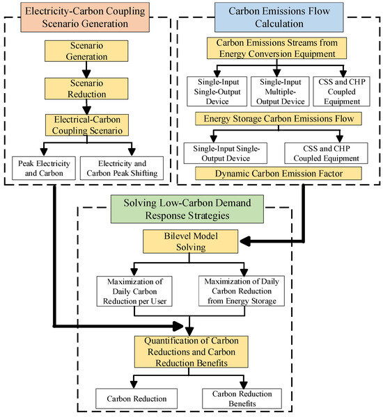
Figure 6. The complete flowchart of the proposed low-carbon demand response strategy.

The solution steps for the low-carbon demand response strategy model proposed in this paper are as follows:

Step 1: Initialise the model by inputting data for the PIES units, energy storage systems, and loads.

Step 2: Obtain 24 h power flow distribution data for the PIES, including line flows and nodal flows.

Step 3: Based on the carbon emission flow theory, calculate the system’s nodal carbon intensity and then use the corresponding formula to determine the dynamic carbon emission factor for each period of the 24 h day.

Step 4: Implement low-carbon demand response for consumers with the objective of maximising their daily carbon reduction. This determines the maximum carbon reduction and corresponding revenue achievable within a dispatch cycle by adjusting consumer electricity consumption patterns.

Step 5: Implement low-carbon demand response for the energy storage system with the objective of maximising its daily carbon reduction. Record the maximum carbon reduction and revenue achieved through the participation of the energy storage unit within the dispatch cycle.

Step 6: Analyse and compare the economic and low-carbon performance across the different scenarios.

5. Case Study

5.1. Parameter Settings

The topological structure of the PIES for the case study is shown in Figure 4, and the parameter settings for each piece of equipment are listed in Table 1. The optimisation model constructed in this paper is a day-ahead centralised optimisation led by the park operator to maximise the total carbon emission reduction of the system. The model is formulated as a mixed-integer linear programming (MILP) problem, which is solved using the CPLEX commercial solver on the MATLAB 2021b platform.

Table 1. Setting of PIES device parameters.

Parameter Name	Setting	Parameter Name	Setting
Coal price	700 CNY/t	Electric boiler	40 MW
Natural gas price	3.5 CNY/m3	Thermal power unit upper/lower output limits	240/80 MW
CHP electric output	125 × 2 MW	Thermal power unit ramp rate	80/−80 MW/h
CHP thermal output	150 × 2 MW	Electrical energy storage capacity and power	100 MWh/20 MW
Gas-fired boiler	80 MW	Thermal energy storage capacity and power	100 MWh/15 MW

Based on the constructed PIES topological structure and specific parameter settings, the corresponding typical scenario curves for “electricity–carbon peak alignment” and “electricity–carbon peak misalignment” are obtained using the methods described in Section 2.1 and Section 2.2, as shown in Figure 7 and Figure 8, respectively. In Figure 7, under the “electricity–carbon peak alignment” scenario, the renewable energy output is at its daily low during the peak load period from 10:00 to 15:00. Concurrently, the peak periods for load and the corresponding carbon emission factor are highly coincident, indicating that the system primarily relies on high-carbon units for power supply during this time, as renewable energy generation is insufficient to meet the load demand. Conversely, in the “electricity–carbon peak misalignment” scenario shown in Figure 8, the carbon emission factor is at a valley during the daytime peak load period (10:00–15:00) due to abundant renewable energy output. However, during the secondary peak load period at night (19:00–21:00), the carbon emission factor climbs to its peak as renewable energy output diminishes, resulting in a temporal misalignment between the electricity consumption peak and the carbon emission peak. Based on these two typical electricity–carbon coupling scenarios, a targeted validation of the proposed low-carbon demand response strategy will be conducted below.

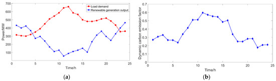
Figure 7. “Electricity–carbon peak alignment” scenario: (a) renewable output and load curves; (b) dynamic carbon emission factor.

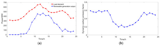
Figure 8. “Electricity–carbon peak misalignment” scenario: (a) renewable output and load curves; (b) dynamic carbon emission factor.

5.2. Analysis of Carbon Emission Reduction from User Participation in Low-Carbon Demand Response

In this paper, the low-carbon benefits brought to the PIES by user participation in low-carbon demand response are validated under the typical scenarios of “electricity–carbon peak alignment” and “electricity–carbon peak misalignment”. The carbon allowance price is set with reference to the projected 2024 domestic carbon market price from reference [22], with an average price of 91.6 CNY/t. For comparison with the results of the low-carbon demand response analysis, the electricity demand response in the case study considers a price-based demand response guided by electricity prices, with the time-of-use (TOU) tariffs shown in Table 2.

Table 2. Time-of-use electricity price.

Time Period		Main-Grid Electricity Price (CNY/kWh)
Peak	08:00–15:00	1.0467
	18:00–21:00
Shoulder	06:00–08:00	0.6821
	15:00–18:00
	21:00–22:00
Off-peak	22:00–next day06:00	0.3782

Figure 9 compares the time-of-use electricity tariff with the dynamic carbon emission factor. Figure 10 illustrates the load changes in the PIES before and after user participation in electricity demand response and low-carbon demand response under the “electricity–carbon peak alignment” scenario. As shown in Figure 10a, under the electricity demand response mechanism guided by electricity prices, users proactively reduce or shift their load from the peak period of 8:00–15:00 to off-peak periods to save on electricity costs. In the “electricity–carbon peak alignment” scenario, the peak electricity consumption period is also the peak carbon emission period. Therefore, the peak-shaving and valley-filling effect of electricity demand response on the load can simultaneously reduce both the energy costs and carbon emissions of the PIES. Figure 10b demonstrates that low-carbon demand response can similarly achieve a peak-shaving and valley-filling effect on carbon emissions. By reducing and shifting the load during the high-carbon period of 8:00–15:00, it also serves to lower the PIES’s electricity costs and carbon emissions. Notably, during the evening peak period of 19:00–21:00, the electricity price is high. However, due to higher renewable energy output at this time, the carbon emission factor is actually low. In this situation, further reducing or shifting the load would be detrimental to the accommodation of renewable energy, leading to a waste of renewable resources. In contrast, low-carbon demand response encourages users to shift their load from the peak carbon emission factor period to the 19:00–21:00 slot, which facilitates the consumption of renewable energy and significantly reduces the PIES’s carbon emissions. Table 3 presents the carbon emission reduction and the corresponding benefits for the PIES under different demand response mechanisms. The data in the table indicate that in the “electricity–carbon peak alignment” scenario, both the carbon emission reduction and the resulting benefits are lower under electricity demand response compared to low-carbon demand response. With low-carbon demand response, the CO₂ emissions from PIES users are reduced by 29.79 tonnes, and the reduction benefits increase by CNY 2729. Therefore, in such scenarios, both electricity prices and carbon emission factors can effectively guide users. While both demand response mechanisms contribute to energy conservation and carbon reduction, low-carbon demand response demonstrates a superior effect in reducing carbon emissions.

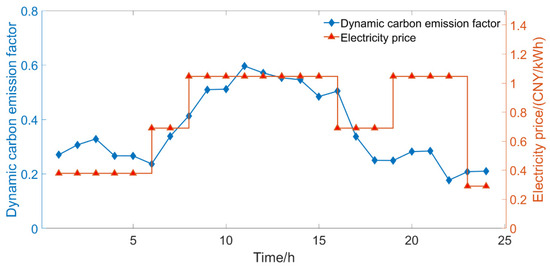
Figure 9. Comparison of dynamic carbon emission factors and TOU in the “electricity–carbon peak alignment” scenario.

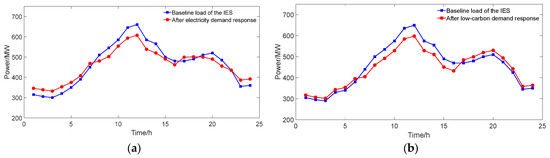
Figure 10. Demand response results in the “electricity–carbon peak alignment” scenario: (a) electricity demand response; (b) low-carbon demand response.

Table 3. Demand response benefits in different scenarios.

Scenario Setting	Electricity–Carbon Peak Alignment		Electricity–Carbon Peak Misalignment
	Emission Reduction/t	Emission-Reduction Benefit/CNY	Emission Reduction/t	Emission-Reduction Benefit/CNY
Electricity demand response	138.69	12,704	62.17	5694
Low-carbon demand response	168.48	15,433	182.25	16,694

Figure 11 shows a comparison between the dynamic carbon emission factor and the electricity price under the “electricity–carbon peak misalignment” scenario. In this scenario, the electricity load and carbon emission intensity within the PIES exhibit different peak and valley characteristics. Particularly during the 0:00–16:00 period, their peaks and valleys are opposite. Consequently, the load curves of PIES users will also change differently under the two demand response mechanisms. As illustrated in Figure 12, in the “electricity–carbon peak misalignment” scenario, the carbon reduction effect of electricity demand response is significantly weakened. This is because, during the off-peak electricity price periods, the load demand is primarily met by high-carbon, high-cost generation units. Shifting excessive load to these off-peak periods would increase the PIES’s energy costs and, simultaneously, its carbon emissions. In contrast, under low-carbon demand response, once users perceive the variations in carbon emissions and the corresponding reduction benefits at different times of the day, they will reduce their electricity consumption during the two high-carbon-factor periods (0:00–7:00 and 19:00–24:00) and shift it to periods with lower carbon emission factors. Observing the load curve after low-carbon demand response, it is evident that an “anti-peak-shaving” phenomenon occurs from 9:00 to 15:00. While this would typically be unfavourable, in this specific context, it is acceptable because renewable energy is at its peak output, and there are sufficient conventional units available as backup capacity in the PIES, ensuring the system remains within safe operational limits. As seen in Table 3, influenced by the “electricity–carbon peak misalignment,” the low-carbon benefits that electricity demand response can bring to PIES users are greatly diminished. Conversely, the equivalent user-side emission reduction and the corresponding benefits generated by low-carbon demand response are enhanced, showing an increase of 120.08 tonnes and CNY 10,999, respectively, compared to electricity demand response. Therefore, in the “electricity–carbon peak misalignment” scenario, the carbon reduction effect of electricity demand response deteriorates, whereas user participation in low-carbon demand response can achieve a higher volume of emission reductions.

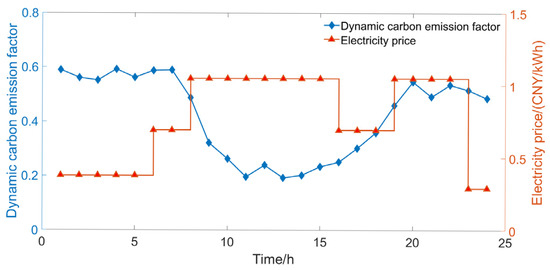
Figure 11. Comparison of dynamic carbon emission factors and TOU in the “electricity–carbon peak misalignment” scenario.

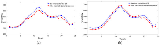
Figure 12. Demand response results in the “electricity–carbon peak misalignment” scenario: (a) electricity demand response; (b) low-carbon demand response.

To further compare the differences between the low-carbon demand response proposed in this paper and conventional electricity demand response, and to analyse the benefits of low-carbon demand response for users from various perspectives, the economic benefit results of the two demand response mechanisms under different scenarios are presented in Table 4. The data in the table show that electricity demand response elicits the largest response volume and yields the highest direct benefits in the “electricity–carbon peak alignment” scenario. In this scenario, the peak electricity price coincides with the peak carbon intensity. Electricity demand response shifts electricity consumption from high-price periods to low-price periods, increasing the response volume by 240 kWh and the response benefits by CNY 1691 compared to low-carbon demand response, thus demonstrating better economic performance. Low-carbon demand response, on the other hand, typically avoids electricity consumption during high-carbon periods and prioritises the use of energy during low-carbon periods. In the “electricity–carbon peak alignment” scenario, low-carbon periods are generally also low-price periods, which allows for considerable economic benefits as well. In the “electricity–carbon peak misalignment” scenario, the load peak occurs precisely when wind and solar power output are abundant. Low-carbon demand response enables the output from these renewable units to meet the load demand. In contrast, electricity demand response, guided by price, often results in the load during off-peak periods being met by high-carbon units. Consequently, under the low-carbon demand response, both the response volume and the response benefits are higher than those under the electricity demand response, with the response volume increasing by 240 kWh and the benefits by CNY 2349.

Table 4. Economic benefits of demand response across different scenarios.

Scenario Setting	Electricity–Carbon Peak Alignment		Electricity–Carbon Peak Misalignment
	Response Energy/MWh	Response Revenue/CNY	Response Energy/MWh	Response Revenue/CNY
Electricity demand response	2.636	18,532	2.169	15,245
Low-carbon demand response	2.396	16,841	2.503	17,594

5.3. Analysis of Carbon Emissions from Energy Storage Participation in Low-Carbon Demand Response

Figure 13 shows the charging/discharging power and state-of-charge (SOC) curves for the energy storage system when participating in low-carbon demand response under the two typical scenarios. As can be seen from the figure, in the “electricity–carbon peak alignment” scenario, the energy storage system primarily charges during periods of abundant renewable energy output and low system carbon intensity, such as 1:00–7:00 and 22:00–23:00. This facilitates the accommodation of surplus green electricity, achieving a temporal shift and storage of low-carbon energy. Conversely, during high-load and high-carbon-intensity periods like 11:00–14:00, the energy storage system discharges in response to the high carbon price signal. This action serves two purposes: it compensates for the power deficit caused by insufficient renewable energy output and peak load, and it effectively reduces the need to dispatch high-carbon marginal units, significantly alleviating the operational and carbon emission pressures on the system. In the “electricity–carbon peak misalignment” scenario, the charging and discharging behaviour of the energy storage system follows the same carbon signal response logic: charging is concentrated during the 11:00–15:00 period, characterised by high renewable energy output and low carbon intensity, while discharging occurs during high-carbon-intensity periods, such as 0:00–5:00 and 20:00–23:00. The consistent charging and discharging behaviour of the energy storage system in both scenarios demonstrates that it effectively achieves a spatiotemporal shift of carbon energy through a “low-carbon charge, high-carbon discharge” model, thereby enhancing the low-carbon performance and economic efficiency of the system’s operation.

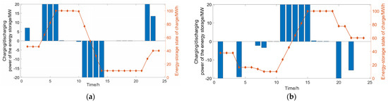
Figure 13. Energy storage charging and discharging behaviour under low-carbon demand response: (a) “electricity–carbon peak alignment” scenario; (b) “electricity–carbon peak misalignment” scenario.

Table 5 presents the benefits of the energy storage system from participating in low-carbon demand response under both scenarios. As shown in the table, under the low-carbon demand response mode, the PIES operator adjusts the charging and discharging behaviour of the energy storage system according to changes in the dynamic carbon emission factor. This can effectively reduce the PIES’s carbon emissions and generate low-carbon benefits. Through the “low-carbon charge, high-carbon discharge” strategy guided by the dynamic carbon emission factor, the energy storage system stores low-carbon electricity during periods of high renewable energy output and low carbon potential and discharges it during high-carbon periods to replace traditional high-carbon power sources. This not only reduces the carbon emission intensity of the PIES but also enhances the efficiency of renewable energy accommodation through synergistic optimisation of electricity and carbon emissions, achieving dual gains in flexibility and low-carbon performance.

Table 5. Low-carbon benefits of energy storage in different scenarios.

Scenario	Emission Reduction/t	Emission-Reduction Benefit/CNY
Electricity–carbon co-peak	21.88	2004
Electricity–carbon peak-shifting	23.90	2189

5.4. Analysis of the Synergistic Relationship Between Users and Energy Storage in Low-Carbon Demand Response

Figure 14a and Figure 14b illustrate the carbon emissions corresponding to the charging and discharging of energy storage systems under two typical scenarios, respectively. In these figures, a positive value on the y-axis represents the charging of the energy storage system, which corresponds to releasing carbon, while a negative value signifies discharging in order to supply power to the load, corresponding to absorbing carbon. This visualisation allows for a direct observation of the changes in carbon emission intensity during different charge–discharge states of the energy storage system, thereby validating the effectiveness of the “carbon carrying capacity” concept in characterising its carbon-related behaviour.

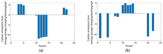
Figure 14. Operational carbon emissions of energy storage: (a) “electricity–carbon peak alignment” scenario; (b) “electricity–carbon peak misalignment” scenario.

Furthermore, by cross-referencing Figure 14 with the renewable energy output and load curves in Figure 7 and Figure 8, as well as the carbon emission trends indicated by the dynamic carbon emission factor for two scenarios, the following observations can be made.

In the “electricity–carbon peak alignment“ scenario, users proactively curtail and shift their load during the high-carbon period of 11:00–15:00. This timeframe also coincides with peak load and insufficient renewable energy generation. During this interval, the energy storage system discharges to supply power to users, compensating for the power deficit and replacing the operation of high-carbon-emitting units, thereby supporting system-wide carbon reduction in a “carbon absorption” state. Conversely, during low-carbon periods with abundant renewable energy, such as 3:00–5:00 and 22:00–23:00, users shift their load from high-carbon periods to these times to enhance renewable energy consumption. The energy storage system also charges during these intervals, collaborating with users to increase the renewable energy accommodation level, thus operating in a “carbon release” state. In the “electricity–carbon peak misalignment” scenario, users shift their load to the low-carbon-intensity period of 11:00–15:00, synergising with the energy storage charging behaviour to consume renewable energy. Meanwhile, during high-carbon periods like 0:00–5:00 and 20:00–23:00, user load reduction and energy storage discharge once again act in concert, reducing the system’s carbon emissions while ensuring power supply. This multi-level coordination between users and the energy storage system, in terms of both timing and response to carbon signals, clearly demonstrates their synergistic relationship in the low-carbon optimisation process.

Overall, in both two scenarios, users and energy storage systems exhibit a significant synergistic relationship when participating in low-carbon demand response. Users indirectly engage in regulation of the system’s carbon flow by dynamically adjusting their electricity consumption behaviour in response to carbon signals—curtailing load during high-carbon periods and increasing usage during low-carbon periods. In contrast, the energy storage system directly modulates the spatiotemporal distribution of carbon flow at the energy conversion stage through intelligent charge–discharge strategies: discharging to replace high-carbon power sources during high-carbon periods and charging to absorb surplus green electricity during low-carbon periods. Acting from the demand side and supply side, respectively, both entities respond to the same carbon price or intensity signal. They coordinate on the temporal scale and complement each other’s regulatory functions, synergistically enhancing the system’s capacity for renewable energy accommodation and its low-carbon operational level. It is within this synergistic relationship that the energy storage system demonstrates regulatory characteristics similar to user response, capable of autonomously adjusting its charging and discharging behaviour based on carbon signals and significantly influencing the system’s carbon footprint. Therefore, an energy storage system can effectively be regarded as a special, highly flexible “virtual user” that actively participates in low-carbon demand response.

6. Conclusions

To effectively reduce the carbon emissions of the PIES, this paper, based on an in-depth exploration of the electricity–carbon coupling relationship, focuses on tapping the carbon emission potential of users and energy storage. A low-carbon demand response strategy is proposed and validated through case studies under two typical electricity–carbon coupling scenarios. The main conclusions are as follows:

(1) An analytical framework based on the typification of electricity–carbon coupling states was proposed. By analysing the correlation mechanism between the system’s carbon flow and its operational state under various combinations of renewable energy output and load, this study is the first to define two typical scenarios: “electricity–carbon peak alignment” and “electricity–carbon peak misalignment”. This approach condenses the continuously evolving electricity–carbon coupling relationship into discrete, highly representative states, deepening our understanding of the key conflicts and mechanisms in the low-carbon operation of multi-energy systems. It also provides a structured scenario basis for the formulation and evaluation of low-carbon demand response strategies.

(2) A coordinated “user plus energy storage” low-carbon demand response strategy centred on a dynamic carbon signal was constructed. By introducing a dynamic carbon emission factor as a unified guiding signal, the strategy not only coordinates user-side load optimisation with the “low-carbon charge, high-carbon discharge” strategy of the energy storage system but also establishes a quantifiable model for assessing carbon reduction and economic benefits. The results validate that this strategy enhances economic efficiency while reducing the system’s carbon emission intensity.

(3) The definition and regulatory dimensions of participants in low-carbon demand response were expanded. This work innovatively defines energy storage as a “virtual user,” transforming it from a passive dispatch object into a key regulatory resource that can autonomously respond to carbon signals based on its electricity consumption characteristics. This not only improves system flexibility but also enhances renewable energy accommodation and carbon reduction effectiveness, offering a new approach for the low-carbon dispatch of PIESs.

(4) Compared to traditional electricity demand response, the proposed low-carbon demand response strategy enhances carbon emission reduction by 21.5% under the “electricity–carbon peak alignment” scenario, and this reduction even doubles under the “electricity–carbon peak misalignment” scenario. Additionally, the integration of energy storage for response increases the park’s average carbon reduction by 15%. This demonstrates that the strategy proposed in this paper significantly improves the park’s capability for carbon emission reduction.

Although this study has yielded some results, it has not yet conducted an in-depth discussion on the impact of other energy forms within the park-level integrated energy system, such as heat and hydrogen, on its overall low-carbon operation. Future work will investigate this aspect further to fully capture the comprehensive influence of the system’s multi-energy coupling and complementarity on its low-carbon operational modes.

Appendix B.1. Carbon Emission Flow Theory: Definitions of Relevant Matrices

(1)

Branch Power Flow Distribution Matrix $P_{\mathrm{B}}={(P_{\mathrm{B}ij})}_{N\times N}$

$$P_{\mathrm{B}ij}=\left\{\begin{array}{cc}{P}_{ij},& P_{ij}>0\\ 0,& P_{ij}\le 0\end{array}\right.$$

(A1)

where P_ij represents the magnitude of power flowing from node i to node j, and N denotes the total number of nodes.

(2)

Source injection distribution matrix $P_{\mathrm{G}}={(P_{\mathrm{G}kj})}_{K\times N}$

$$P_{\mathrm{G}kj}=\left\{\begin{array}{cc}{P}_k,& k,j\in G_{kj}\\ 0,& k,j\notin G_{kj}\end{array}\right.$$

(A2)

where P_k denotes the injection power from source k, G_kj represents the source set indicating the connection of source k to node j, and k is the total number of sources.

(3)

Load distribution matrix $P_{\mathrm{L}}={\left(P_{\mathrm{L}mj}\right)}_{M\times N}$

$$P_{\mathrm{L}mj}=\left\{\begin{array}{cc}{P}_{\mathrm{load},mj},& m,j\in M_{mj}\\ 0,& m,j\notin G_{kj}\end{array}\right.$$

(A3)

where P_load,mj represents the power magnitude of load m, M_mj denotes the load set indicating the connection of load m to node j, and M is the total number of loads.

(4)

Node flux matrix $P_{\mathrm{N}}$

$$P_{\mathrm{N}}=diag\left({\xi }_{N+K}\left[\begin{array}{c}{P}_B\\ P_G\end{array}\right]\right)$$

(A4)

where the diagonal elements in P_N represent the total inflow power at each node, and ξ_N+K denotes a row vector with all elements equal to unity.

(5)

Source-side carbon emission factor vector $E_{\mathrm{G}}$

$$E_{\mathrm{G}}={\left[\begin{array}{cccc}{e}_{\mathrm{G}1},& e_{\mathrm{G}2},& \cdots ,& e_{\mathrm{G}k}\end{array}\right]}^{\mathrm{T}}$$

(A5)

where e_Gk denotes the carbon emission factor of source k.

Appendix B.2. Calculation Formula for the Dynamic Carbon Emission Factor Matrix

(1)

Node carbon emission intensity vector $E_N$

$$E_N={\left(P_N-P_{\mathrm{B}}^{\mathrm{T}}\right)}^{-1}{P}_{\mathrm{G}}^{\mathrm{T}}{E}_{\mathrm{G}}$$

(A6)

(2)

Branch carbon flow rate distribution matrix $R_{\mathrm{B}}$

$$R_{\mathrm{B}}=P_{\mathrm{B}}diag\left(E_N\right)$$

(A7)

(3)

Load carbon flow rate vector $R_{\mathrm{L}}$

$$R_{\mathrm{L}}=P_{\mathrm{L}}{E}_N$$

(A8)

Appendix B.3. Computational Formula for Node-Level Carbon Intensity in Electricity, Gas, and Heating Networks of PIES

The computational formula for carbon emission intensity at grid nodes is expressed as

$$e_{e,i}^N={\displaystyle \frac{{\displaystyle \sum _{i\in N}{P}_{\mathrm{PG},i}{e}_{e,\mathrm{G}}}+{\displaystyle \sum _{l\in {\Omega }_{e,in}^i}{P}_{\mathrm{e},l}{e}_{e,l}^B}}{{\displaystyle \sum _{i\in N}{P}_{\mathrm{PG},i}}+{\displaystyle \sum _{l\in {\Omega }_{e,in}^i}{P}_{\mathrm{e},l}}}}$$

(A9)

where $e_{e,i}^N$ represents the carbon emission intensity at grid node i; $e_{e,l}^B$ denotes the carbon emission intensity of branch l; $e_{e,\mathrm{G}}$ indicates the carbon emission intensity of power generation units; $P_{\mathrm{PG},i}$ corresponds to the active power on branch l; and ${\Omega }_{e,in}^i$ signifies the set of branches flowing into node i.

The calculation formula for nodal carbon intensity in district heating networks is expressed as

$$e_{h,i}^N={\displaystyle \frac{{\displaystyle \sum _{i\in N}{P}_{\mathrm{HS},i}{e}_{h,\mathrm{S}}}+{\displaystyle \sum _{l\in {\Omega }_{h,in}^i}{P}_{h,l}{e}_{h,l}^B}}{{\displaystyle \sum _{i\in N}{P}_{\mathrm{HS},i}}+{\displaystyle \sum _{l\in {\Omega }_{h,in}^i}{P}_{h,l}}}}$$

(A10)

where $e_{e,i}^N$ denotes the carbon emission intensity at heating network node i; $e_{h,l}^B$ represents the carbon emission intensity of pipeline l; $e_{h,\mathrm{S}}$ indicates the carbon emission intensity of heat supply units; $P_{\mathrm{HS},i}$ corresponds to the thermal power supplied by the heat source at node i; $P_{h,l}$ refers to the equivalent thermal power on pipeline l; and ${\Omega }_{h,in}^i$ signifies the set of pipelines flowing into node i.

The computational formula for nodal carbon intensity in natural gas networks is given by

$$e_{g,i}^N={\displaystyle \frac{{\displaystyle \sum _{i\in N}{P}_{\mathrm{GS},i}{e}_{g,\mathrm{S}}}+{\displaystyle \sum _{l\in {\Omega }_{g,in}^i}{P}_{g,l}{e}_{g,l}^B}}{{\displaystyle \sum _{i\in N}{P}_{\mathrm{GS},i}}+{\displaystyle \sum _{l\in {\Omega }_{g,in}^i}{P}_{g,l}}}}$$

(A11)

where $e_{g,i}^N$ represents the carbon emission intensity at gas network node i; $e_{g,l}^B$ denotes the carbon emission intensity of pipeline l; $e_{g,\mathrm{S}}$ indicates the carbon emission intensity of gas sources; $P_{\mathrm{GS},i}$ corresponds to the equivalent power of the gas source at node i; $P_{g,l}$ refers to the equivalent power on pipeline l; and ${\Omega }_{g,in}^i$ signifies the set of pipelines flowing into node i.

References

- Sun, S.; Xing, J.; Cheng, Y.; Yu, P.; Wang, Y.; Yang, S.; Ai, Q. Optimal Scheduling of Integrated Energy System Based on Carbon Capture-Power to Gas Combined Low-Carbon Operation. Processes 2025, 13, 540. [Google Scholar] [CrossRef]
- Liu, J.; Ma, L.; Wang, Q. Energy Management Method of Integrated Energy System Based on Collaborative Optimization of Distributed Flexible Resources. Energy 2023, 264, 12598. [Google Scholar] [CrossRef]
- Guo, Y.; Wang, Q.; Wang, M.; Wang, Z.; Liu, Y.; Chen, Y. Low-carbon economic operation strategy of park integrated energy system considering carbon flow optimization. Electr. Power Eng. Technol. 2025, 44, 64–75. [Google Scholar] [CrossRef]
- Yang, C.; Dong, X.; Wang, G.; Lv, D.; Gu, R.; Lei, Y. Low-carbon economic dispatch of integrated energy system with CCS–P2G–CHP. Energy Rep. 2024, 12, 42–51. [Google Scholar] [CrossRef]
- Li, X.; Liu, L.; Hang, J.; Wu, X.; Li, H.; Chen, Y. Optimal scheduling of park-level integrated energy system with coupling of P2G and CCS. Proc. CSU-EPSA 2023, 35, 18–25. [Google Scholar] [CrossRef]
- Chantzis, G.; Giama, E.; Nižetić, S.; Papadopoulos, A.M. The potential of demand response as a tool for decarbonization in the energy transition. Energy Build. 2023, 296, 113255. [Google Scholar] [CrossRef]
- Li, Y.; Han, M.; Shahidehpour, M.; Li, J.; Long, C. Data-driven distributionally robust scheduling of community integrated energy systems with uncertain renewable generations considering integrated demand response. Appl. Energy 2023, 335, 120749. [Google Scholar] [CrossRef]
- Lyu, X.; Liu, T.; Liu, X.; He, C.; Nan, L.; Zeng, H. Low-carbon robust economic dispatch of park-level integrated energy system considering price-based demand response and vehicle-to-grid. Energy 2023, 263, 125739. [Google Scholar] [CrossRef]
- Cai, C.; He, Y.; Shi, Q.; Hou, H.; Wang, B. Low-carbon optimal dispatching of hydrogen-containing IES considering joint green certificate–carbon emission trading and demand response. Electr. Power Eng. Technol. 2025, 44, 43–52. [Google Scholar] [CrossRef]
- Li, Y.; Zhang, N.; Du, E.; Liu, Y.; Cai, X.; He, D. Mechanism study and benefit analysis on power system low-carbon demand response based on carbon emission flow. Proc. CSEE 2022, 42, 2830–2842. [Google Scholar] [CrossRef]
- Ye, Y.; Xing, H.; Mi, Y.; Yan, Z.; Dong, J. Low-carbon optimal dispatching of integrated energy system considering low-carbon demand response and Stackelberg game. Autom. Electr. Power Syst. 2024, 48, 34–43. [Google Scholar] [CrossRef]
- Yang, Z.; Xing, H.; Jiang, W.; Wang, H.; Sun, Y.; Yan, Z. Optimal scheduling of integrated energy system with coal-to-hydrogen and carbon capture power plant based on low-carbon demand response. Electr. Power Autom. Equip. 2024, 44, 25–32. [Google Scholar] [CrossRef]
- Zhang, X.; Wang, L.; Huang, L.; Wang, S.; Wang, C.; Guo, C. Optimal dispatching of park-level integrated energy system considering augmented carbon emission flow and carbon trading bargain model. Autom. Electr. Power Syst. 2023, 47, 34–46. [Google Scholar] [CrossRef]
- Yang, M.; Zhu, Y.; Yu, X.; SU, X.; Wang, Y.; Wang, J.; Liu, J. Distributionally robust low-carbon scheduling of integrated energy system considering source–load collaborative carbon reduction under multiple time scales. Electr. Power Autom. Equip. 2025, 45, 34–45. [Google Scholar] [CrossRef]
- Liu, H.; Li, H.; Ma, J.; Chen, J.; Zhang, W. Distributionally robust optimal dispatching of integrated electricity and heating system considering source–load uncertainty. Electr. Power Autom. Equip. 2023, 43, 1–8. [Google Scholar] [CrossRef]
- Mu, C.; Zhang, J.; Cheng, C.; Xu, Y.; Yang, Y. High-dimensional uncertainty scenario generation method for hydro–wind–solar multi-energy complementary system considering spatio-temporal correlation. Power Syst. Technol. 2024, 48, 3614–3623. [Google Scholar] [CrossRef]
- Zhao, S.; Zhao, P.; Wei, Z.; Liao, Y.; Wang, Z. Multi-scenario stochastic optimal scheduling considering multi-prediction error band information under data-driven. Electr. Power Autom. Equip. 2024, 44, 52–59. [Google Scholar] [CrossRef]
- Cheng, Y.; Guo, X.; Liu, Q. Quantification model of carbon emission reduction benefits based on dynamic carbon emission factors in a substation area. Mod. Electr. Power 2025, 42, 168–175. [Google Scholar] [CrossRef]
- Cui, Y.; Zou, X.; Zhao, Y.; Fu, X.; Shen, Y. Electricity–carbon integrated demand response scheduling method for new power system considering dynamic electricity–carbon emission factor. Electr. Power Autom. Equip. 2024, 44, 1–7. [Google Scholar] [CrossRef]
- Zhou, T.; Kang, C.; Xu, Q.; Chen, Q. Preliminary investigation on a method for carbon emission flow calculation of power system. Autom. Electr. Power Syst. 2012, 36, 44–49. [Google Scholar] [CrossRef]
- Cheng, Y.; Zhang, N.; Wang, Y.; Yang, J.; Kang, C.; Xia, Q. Modeling Carbon Emission Flow in Multiple Energy Systems. IEEE Trans. Smart Grid 2019, 10, 3562–3574. [Google Scholar] [CrossRef]
- Wang, K.; Lü, C. Review and outlook of global and China’s carbon markets. J. Beijing Inst. Technol. (Soc. Sci. Ed.) 2025, 27, 19–36. [Google Scholar] [CrossRef]
Disclaimer/Publisher’s Note: The statements, opinions and data contained in all publications are solely those of the individual author(s) and contributor(s) and not of MDPI and/or the editor(s). MDPI and/or the editor(s) disclaim responsibility for any injury to people or property resulting from any ideas, methods, instructions or products referred to in the content. |
© 2025 by the authors. Licensee MDPI, Basel, Switzerland. This article is an open access article distributed under the terms and conditions of the Creative Commons Attribution (CC BY) license (https://creativecommons.org/licenses/by/4.0/).