Numerical Simulation on the Propagation Behaviour of Hydraulic Fractures in Sandstone–Shale Interbeds

Abstract

In the shale oil reservoirs, sandstone and shale often overlie each other. This significantly affects the vertical propagation of hydraulic fractures (HFs); however, the underlying mechanisms still remain unclear. This study employs Xsite software to investigate the influence of rock fracture toughness, tensile strength, elastic modulus, Poisson’s ratio, interlayer stress contrast, and the flow rate and viscosity of fracturing fluid on the propagation behaviour of HFs in sandstone–shale interbeds. As the type-I fracture toughness of the shale layer increases, the area of the vertical HF decreases and the average HF width becomes smaller. As the tensile strength of the sandstone layer increases, the distribution range of fluid pressure at the interface expands. The HF prefers to propagate in the softer rock rather than the harder one. A relatively narrower HF width is created in the layer with a higher elastic modulus resulting in a higher flow resistance to fracturing fluid. A shale layer with a high Poisson’s ratio is more likely to undergo a lateral expansion, causing stress at the fracture tip to be dispersed. When the effect of lithological interfaces is considered, an increasing interlayer stress contrast causes HFs to gradually transition from penetrating the interfaces to becoming confined between the two interfaces. When the influence of the lithological interface is not considered, an increasing interlayer stress contrast causes the HF to gradually transition from a penny-shaped fracture to a blade-shaped fracture. The HF penetrates the interfaces more easily at a higher injection rate and fluid viscosity, because most of the injected energy is used to create new fractures rather than leakoff into the interfaces. Understanding the influence of these factors on the HF propagation behaviour is of great significance for optimising hydraulic fracturing design.

1. Introduction

Complex layered rock develops in the formation of shale oil reservoirs, exhibiting significant stratigraphic heterogeneity. This heterogeneity restricts the vertical propagation of hydraulic fractures (HFs), making it difficult to achieve the desired outcomes in reservoir stimulation.

The study of the HF geometry in complex-layered shale reservoirs is a hot topic in the field of oil and gas development. Tan and Liao [1,2] conducted a series of triaxial fracturing experiments on shale outcrops and established a finite element model of hydraulic fracturing in layered shale reservoirs. They indicated that the strength characteristics of lithological interfaces have a significant impact on HF propagation. The stronger the laminar cohesive force and rock interface properties, the easier it is for HFs to cross the rock interface [3,4]. A decrease in bedding shear strength enhances the ability of HFs to divert [5]. Li et al. and Lu et al. [6,7] indicated that the dip angle of the lithological interface also affects the vertical propagation behaviour of HFs. It is more likely to penetrate vertically through interface with a lower dip angle. Zhao et al. [8] concluded that some geological and engineering parameters control the cross-layer propagation behaviour of HFs in continental shale reservoirs, including the in situ stress contrast, elastic modulus contrast, and fracturing fluid parameters. Among these, the in situ stress contrast is the most significant factor affecting the vertical propagation behaviour of HFs [9,10]. The smaller the stress contrast between layers, the greater probability for the HF to penetrate the rock interface [11,12]. Tang et al. [13] studied the interaction between multiple HFs and bedding planes and found that the bedding plane induces shear slip in HFs. Ma et al. [14] studied the effects of elastic modulus, the Poisson’s ratio, and other factors on HF propagation. Higher values of elastic modulus and Poisson’s ratio make it easier for HF to form, and a higher Poisson’s ratio results in faster HF propagation. High fracturing fluid injection rates and high viscosity are conducive to the vertical growth of HFs [15,16,17]. In addition, the interlayer permeability difference, filtration loss coefficient, perforation parameter, and interlayer friction coefficient also exert a certain degree of influence on the vertical propagation of HFs in shale reservoirs. In addition to the traditional physics-driven method, artificial neural networks and machine learning are new trends in HF simulation within reservoirs [18].

In summary, the above-mentioned studies mainly focus on a single factor which affects the HF geometry. However, the actual propagation behaviour of HFs is not controlled by a single factor but is the result of the combined influence of factors such as interlayer stress conditions, rock mechanical properties, and fracturing fluid parameters [4]. Furthermore, the influence on HF propagation varies significantly depending on the combination of different formation conditions. Therefore, this paper investigates the influence of factors such as rock mechanical properties, interlayer stress, and fracturing fluid properties on the vertical propagation behaviour of HF in sandstone–shale interbeds.

2. Numerical Model Building and Validation

2.1. HF Model Building

XSite (Version 3.0.53) is a commercial software used for hydraulic fracturing simulation based on the discrete lattice method [19]. It simplifies the bonded particle model into a lattice network, where each node in the network represents a particle in the bonded particle model and the springs represent the contacts between particles. One of the most apparent weaknesses of the discrete lattice method is computation speed because of the extensive particles and springs among them. The others are the scaling and resolution effects because the geometry size of HF in this method is on the order of 10 m, whereas the actual HF is usually on the order of 100 m. Pipe network is used to connect fluid units and the pipeline length represents the HF width, which is different from the conventional HF model.

2.1.1. Solid Mechanics Equations Due to HF Deformation

Rocks are represented by a series of nodes connected by the springs. Each node possesses three translational and three rotational freedom degrees. The translational freedom degrees of the nodes are calculated using Newton’s second law:

$${\dot{u}}_i^{\left(t+\Delta t/2\right)}={\dot{u}}_i^{\left(t-\Delta t/2\right)}+\left(\sum F_i^{\left(t\right)}\right){\displaystyle \frac{\Delta t}{m}}$$

(1)

$$u_i^{\left(t+\Delta t\right)}=u_i^{\left(t\right)}+{\dot{u}}_i^{\left(t+\Delta t/2\right)}\Delta t$$

(2)

where ${\dot{u}}_i^{(t)}$ is the velocity at time t in the i-component, m/s and $u_i^{(t)}$ is the t-momentum displacement in the i-component, m. m is the mass, Kg. F_i is force of the i-component, N and ∆t is the time increment, s.

The angular velocity of node component i (i = 1, 2, 3) at the moment t is given by:

$${\omega }_i^{\left(t+\Delta t/2\right)}={\omega }_i^{\left(t-\Delta t/2\right)}+{\displaystyle \frac{\sum M_i^{\left(t\right)}}{I}}\Delta t$$

(3)

where $\sum M_i^{\left(t\right)}$ is the sum of all i-component moments, N·m, and I is the inertia moment, kg·m². ${\omega }_i$ is the angular velocity, rad/s.

The normal force and shear stress of springs are expressed as:

$$\left\{\begin{array}{l}{F}_i^N\leftarrow F_i^N+{\dot{u}}_i^N{k}^N\Delta t\\ F_i^S\leftarrow F_i^S+{\dot{u}}_i^S{k}^S\Delta t\end{array}\right.$$

(4)

where k^N and k^S are normal and tangential spring stiffness, respectively, N/m and F_i^N and F_i^S are normal and tangential forces at the moment t, respectively, N. ${\dot{u}}_i^N$ and ${\dot{u}}_i^S$ are normal and tangential velocities, respectively, m/s.

The relationship between the elastic characteristics of microscopic springs and macroscopic rock bodies is expressed as follows:

$$\left\{\begin{array}{l}{F}^{N\max }={\alpha }_{t}T{R}^2\\ F^{S\max }=\mu F^{N\max }+{\alpha }_{s}C{R}^2\end{array}\right.$$

(5)

where F^Nmax and F^Smax are the tensile and shear strengths of the spring, respectively, N; α_t and α_s are the tensile and shear strength correction factors, respectively; T and C are the rock tensile and shear strengths, respectively, Pa; R is the unit dimension, m; and μ is the frictional coefficient, dimensionless.

2.1.2. Fluid Flow Equations Inside the HF

The flowing fluid is simulated by using pipe networks to connect fluid units, which are positioned at the centres of broken springs or spring joints. Newly formed microcracks are automatically integrated into the pipe networks.

Based on the lubrication equation and the assumption that the pipeline length equals its width, the formula to calculate the fluid flow rate from node A to B along the pipeline is as follows [19]:

$$q=\beta k_r{\displaystyle \frac{a^3}{12\mu }}\left[p_{\mathrm{A}}-p_{\mathrm{B}}+{\rho }_{W}g(z_{\mathrm{A}}-z_{\mathrm{B}})\right]$$

(6)

where β is the calibration coefficient, dimensionless; a is the HF width, m; μ is the liquid viscosity, Pa·s; p is the fluid pressure at the node, Pa; ρ_w is the fluid density, kg/m³; z_A and z_B are the hydraulic head at the nodes A and B, respectively, m; and k_r is the relative permeability. p_A and p_B are the pressure at the nodes A and B, respectively, and Pa. g is the gravity acceleration, m/s².

The formula to calculate the fluid pressure increment at each time step is as follows:

$$\Delta P={\displaystyle \frac{Q}{V}}{K}_f\Delta t$$

(7)

where Q is the summation of all flow rates, m³/s; V is the node volume, m³; and K_f is the apparent fluid bulk modulus, Pa.

2.1.3. Fluid‒Solid Coupling Method

The fluid initially flows through the HF and gradually infiltrates the rock matrix. This process involves the dynamic properties of the fluid. The fluid infiltrating the rock matrix alters the mechanical and fundamental properties of the rock, thereby influencing the characteristics of the HF, which in turn affects certain properties of the fluid. Ultimately, this feedback loop further impacts the fluid’s flow within the HF. Therefore, the solid mechanics equation and the fluid flow equation are mutually coupled and exert reciprocal influence.

2.2. HF Model Validation

Huang et al. [20] used an artificial cement sample to simulate the propagation behaviour of HF and analysed the influence of bedding plane characteristics and stress conditions on the HF propagation [20]. This paper adopts the same parameters (see Table 1) to conduct numerical simulation. The HF geometry of the numerical simulation is given in Figure 1a. Due to variations in interlayer mechanical properties (e.g., the interface tensile strength is much less than the rock tensile strength), the HFs exhibit markedly discontinuous expansion when crossing the interface. A small part of fracturing fluid leaks off in the interface when the HF crosses the interface. The HF shape and area both agree with Huang’s experiment [20]. During the radial propagation of HFs at the beginning, the HF’s width and radius are both slightly less than the analytical solutions of radial HF, respectively, as shown in Figure 1b. One cause is that the fluid leakoff process in this model is completely different from the Carter’s leakoff used in the analytical solution of the radial HF. Another cause is probably the fracture tip behaviour.

Table 1. Input parameters.

Parameters	Value	Parameters	Value
Density (g/cm3)	3.10	Fracturing fluid injection rate (m3/min)	10.00
Elastic modulus (GPa)	0.72	Maximum horizontal principal stress (MPa)	36.00
Poisson’s ratio (dimensionless)	0.13	Minimum horizontal principal stress (MPa)	32.00
Uniaxial compressive strength (MPa)	6.27	Vertical principal stress (MPa)	38.00
Rock tensile strength (MPa)	1.65	Interface friction angle (°)	31.29
Type-I fracture toughness (MPa·m1/2)	1.32	Interface cohesion (MPa)	2.54
Fracturing fluid viscosity (mPa·s)	3.00	Interface tensile strength (MPa)	0.43
Fracturing fluid density (g/cm3)	1.20

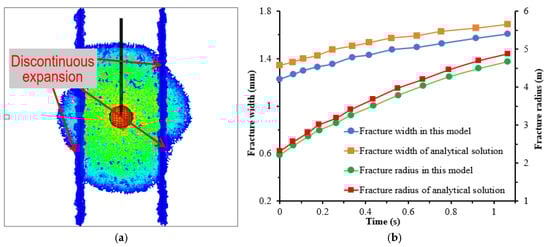
Figure 1. Numerical simulation in this model for validation. (a) HF geometry when crossing the interface. (b) Comparisons with the analytical solutions of radial HF.

3. Modelling of HF Propagation

3.1. Geometry Model and Input Parameters

The HF propagation behaviour of a sandstone–shale interbed is simulated to study the influence of various factors on the morphology of HF. A basic model comprising three rock layers and two interfaces is established in Figure 2. Its dimensions are 20 × 20 × 20 m. A 6 m-long horizontal wellbore is placed at the centre of the shale layer, with the perforation located at the wellbore centre. The basic parameters of the model are given in Table 2, which are adopted in all the subsequent numerical simulations.

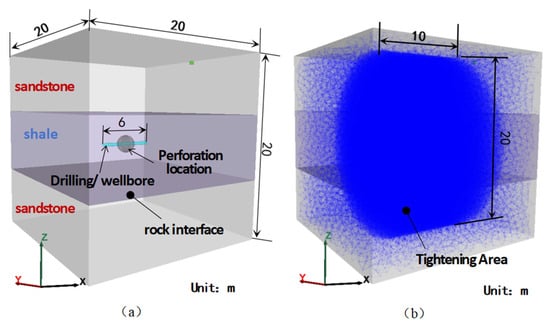
Figure 2. Geometry model (a) and the discrete lattice model (b).

Table 2. Parameter settings of the model.

Parameters	Sandstone	Shale	Parameters	Value
Density (g/cm3)	2.3	2.7	Fracturing fluid density (g/cm3)	1.2
Elastic modulus (GPa)	25.0	14.0	Fracturing fluid viscosity (mPa·s)	3.00
Poisson’s ratio (dimensionless)	0.2	0.3	Fracturing fluid injection rate (m3/min)	10.00
Uniaxial compressive strength (MPa)	200.0	100.0	Interface tensile strength (MPa)	0.50
Tensile strength St (MPa)	4.8	2.0	Interface cohesion (MPa)	0.90
Type-I fracture toughness KIC (MPa·m1/2)	0.3	0.8	Interface friction angle (°)	30.00
Porosity (%)	2.0	6.0	Interface opening degree (m)	0.0001
Permeability (mD)	0.3	0.6
Maximum horizontal principal stress (MPa)	22.0	20.0
Minimum horizontal principal stress (MPa)	17.0	15.0
Vertical principal stress (MPa)	25.0	25.0

3.2. The Influence of Tensile Strength and Type-I Fracture Toughness

The type-I fracture toughness (labelled as K_IC) and the corresponding tensile strength (labelled as S_t) for the shale and sandstone layers were determined according to the empirical formulas proposed by Whittaker et al. [21] and Deng et al. [22], respectively, as shown in Table 3. Other parameters are listed in Table 2. According to Equation (6), the pipe length equals the width of the HF. The width and fluid pressure of the HF according to the numerical simulations are given in Figure 3 and Figure 4.

Table 3. Parameter settings for type-I fracture toughness and tensile strength of rock.

Rock	Reference	Empirical Formula	KIC (MPa·m1/2)	St (MPa)
shale	Ref. [21]	$S_t=9.35 K_{\mathrm{IC}}-2.53$	0.3	0.275
			0.7	4.015
			1.1	7.755
			1.5	11.495
sandstone	Ref. [22]	$r={\displaystyle \frac{1}{2\pi }}{\left({\displaystyle \frac{K_{\mathrm{IC}}}{S_{\mathrm{t}}}}\right)}^2{\left[\cos {\displaystyle \frac{\theta }{2}}\left(1+\sin {\displaystyle \frac{\theta }{2}}\right)\right]}^2$ $S_t=K_{\mathrm{IC}}/\sqrt{2\pi r}$	0.219	3.5
			0.313	5.0
			0.406	6.5
			0.500	8.0

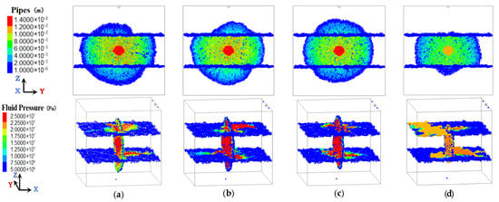
Figure 3. HF propagation patterns and fluid pressure distribution under different fracture toughness of shale. (a) 0.3 MPa·m^1/2. (b) 0.7 MPa·m^1/2. (c) 1.1 MPa·m^1/2. (d) 1.5 MPa·m^1/2.

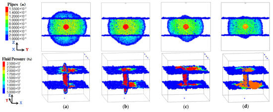
Figure 4. HF propagation patterns and fluid pressure distribution under different tensile strengths of sandstone. (a) 3.5 MPa. (b) 5.0 MPa. (c) 6.5 MPa. (d) 8.0 MPa.

As shown in Figure 3, when the type-I fracture toughness (K_IC) of the shale layer is less than 1.1 MPa·m^1/2, the distribution range of fluid pressure at the interface is limited around the contact area, whereas the fluid pressure values at the injection points are greater than 25 MPa (the vertical principal stress) resulting in the HF penetrating both the upper and lower interfaces. As the type-I fracture toughness of the shale layer increases, the distribution range of fluid pressure at the interface expands, but the fluid pressure values at the injection points decrease. As the type-I fracture toughness of the shale layer increases, the area of the vertical HF decreases and the average HF width becomes smaller.

As shown in Figure 4, when the tensile strength (S_t) of the sandstone layer is less than 3.5 MPa, the vertical main HF is approximately circular. As the tensile strength of the sandstone layer increases, the distribution range of fluid pressure at the interface expands, but the fluid pressure at the injection point decreases. Once the fluid pressure at the injection point is less than 25 MPa (vertical principal stress), the interface cannot be open, resulting in the HF being limited in the shale layer. In addition, the tensile strength of the interface is usually less than the shale or sandstone matrix, a small part of fracturing fluid will prefer to diffuse along the interface and not open the interface.

3.3. The Influence of Shale’s Elastic Modulus and Poisson’s Ratio

Only the elastic modulus (8 GPa,16 GPa, 24 GPa, and 32 GPa) and the Poisson’s ratio (0.2, 0.25, 0.3, and 0.35) of the shale layer vary, the remaining parameters are in Table 2, and the simulation results are given in Figure 5 and Figure 6.

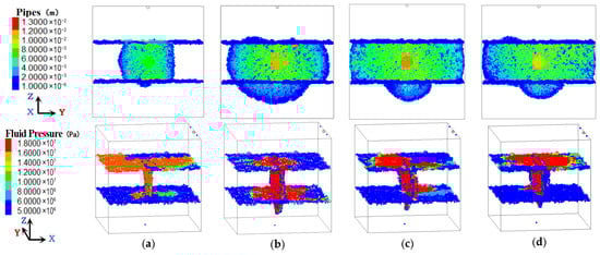
Figure 5. HF patterns and fluid pressure distribution under different shale elastic moduli. (a) 8 GPa. (b) 16 GPa. (c) 24 GPa. (d) 32 GPa.

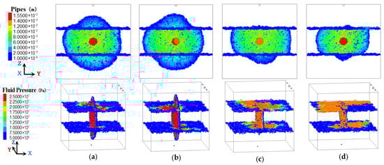
Figure 6. HF patterns and fluid pressure distribution under different shale Poisson’s ratios. (a) 0.2. (b) 0.25. (c) 0.3. (d) 0.35.

As shown in Figure 5, when the elastic modulus of the shale layer is less than 8 GPa, the height of the HF is limited to the shale layer and it cannot cross the interlayer. The reason is that the elastic modulus of the sandstone layer is 25 GPa, which is much greater than the elastic modulus of the shale layer. When the elastic modulus of the shale layer is greater than 25 GPa, the HF can cross the interlayer easily. It indicates that the HF prefers to propagate in the softer layer rather than the harder one. If the shale layer is much harder than the sandstone layer in the actual reservoir, the HF will shift to the sandstone layer even though the injected point locates in the shale layer. In contrast, if the shale layer is much softer than the sandstone layer, the HF will be fully restrained in the shale layer. A relatively narrower HF width is created in the harder layer, resulting in a higher flow resistance of fracturing fluid and a higher fluid pressure inside the HF and lithological interface.

As shown in Figure 6, as the Poisson’s ratio of the shale layer increases, the HF gradually shifts from penetrating both the upper and lower interfaces to penetrating only the lower interface. The cross-layer area decreases, while the HF width increases slightly. When the Poisson’s ratio is 0.2 or 0.25, the fluid pressure distribution at the interface is similar, exhibiting a smaller distribution range but higher fluid pressure at the injection point. As the Poisson’s ratio of shale increases, the distribution range of fluid pressure at the interface expands, while the fluid pressure at the interface decreases.

Low elastic modulus is characterised by low stiffness and high fracture toughness. The fluid energy released during fracture propagation is extensively absorbed, thereby limiting fracture growth. In contrast, rock layers with a high elastic modulus exhibit high stiffness and brittleness. Once the HF forms, stress concentration at the HF’s tip becomes pronounced, leading to accelerated fracture propagation and ultimately a larger HF. A low Poisson’s ratio results in a reduced lateral deformation capacity, with energy more concentrated in vertical deformation. Therefore, the HF tends to extend vertically, making them more prone to penetrate the interlayer. In contrast, a shale layer with a high Poisson’s ratio is more likely to undergo a lateral expansion, causing stress at the HF tip to be dispersed.

According to Section 3.2 and Section 3.3, a simple sensitivity analysis showing the impact of the rock’s mechanical properties on the HF’s penetration behaviour is given in Figure 7.

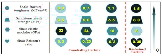
Figure 7. Impact of the rock’s mechanical properties on fracture penetration.

3.4. The Influence of Interlayer Stress

The principal stress of the shale layer keeps consistent with Table 2, while the stress of the sandstone layer is modified, as shown in Table 4. The remaining parameters are in Table 2. Two scenarios are simulated: one considering the influence of lithological interface properties (i.e., taking into account the tensile strength, cohesion, and internal friction angle of the interface), and another disregarding these effects. Disregarding the effects of lithological interface properties means that the interface is still perfectly bonded when the HF penetrates both the upper and lower interfaces. Under this condition, the HF will not open the lithological interface. The simulation results are presented in Figure 8 and Figure 9.

Table 4. Ground stress settings in sandstone formations.

Interlayer Stress Contrast (MPa)	Maximum Horizontal Principal Stress (MPa)	Minimum Horizontal Principal Stress (MPa)	Vertical Principal Stress (MPa)
1	21	16	25
2	22	17	25
4	24	19	25
8	28	23	25

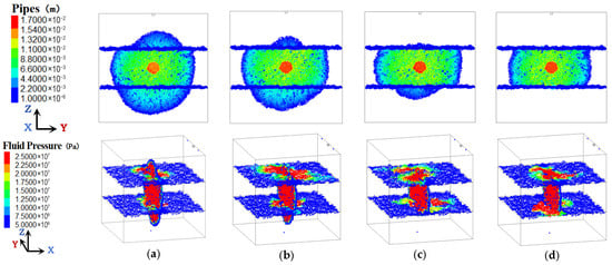
Figure 8. HF propagation morphology and fluid pressure distribution under varying interlayer stress contrasts (considering lithological interfaces). (a) 1 MPa. (b) 2 MPa. (c) 4 MPa. (d) 8 MPa.

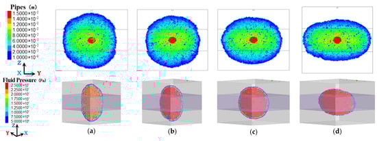
Figure 9. HF propagation morphology and fluid pressure distribution under varying interlayer stress contrasts (without considering the lithological interface). (a) 1 MPa. (b) 2 MPa. (c) 4 MPa. (d) 8 MPa.

As shown in Figure 8, when the effects of lithological interfaces are considered, an increasing interlayer stress contrast causes the HF to gradually transition from penetrating both the upper and lower interfaces to penetrating only the lower interface and eventually becoming confined between the two interfaces. The HF width gradually increases, and both the magnitude and distribution range of fluid pressure increase along the two interfaces. The leakoff area of the fracturing fluid along the lithological interfaces also expands. When the interlayer stress contrast becomes sufficiently large (e.g., larger than 8 MPa in Figure 8d), the fracturing fluid flows almost entirely along the lithological interface and the HF height equals the thickness of the shale layer.

As shown in Figure 9, when the influence of the lithological interface is not considered, the morphology of the HF is generally smoother. As the interlayer stress contrast increases, the HF height gradually decreases, while the HF width gradually increases. The shape of HF gradually transitions from a penny-shaped fracture to a blade-shaped fracture. It is inferred that when the interlayer stress contrast is sufficiently large (e.g., larger than 8 MPa in Figure 9d), the expansion region of the HF is almost confined in the shale layer, resulting in a “stress barrier” phenomenon. For the practical fracturing treatments, if the minimum principal stress is along the horizontal direction, the vertical propagation of the HF is highly restrained by the stress barrier. A critical value of stress contrast may exist to prevent the HF from crossing the interface.

3.5. The Influence of Fracturing Fluid Injection Rate and Viscosity

By keeping the total injected volume of fracturing fluid constant, with parameter settings as shown in Table 2, the simulation results for HF cross-layer propagation at different fracturing fluid flow rates (5 m³/min, 10 m³/min, 15 m³/min) are shown in Figure 10. The HF propagates through the formation under different fracturing fluid viscosities (2 mPa·s, 4 mPa·s, 10 mPa·s, and 30 mPa·s), which are shown in Figure 11.

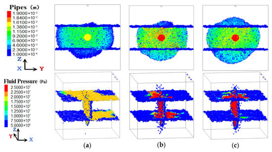
Figure 10. HF morphology and fluid pressure distribution at different injection rates. (a) 5 m³/min. (b) 10 m³/min. (c) 15 m³/min.

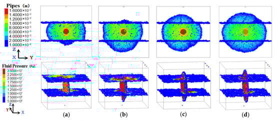
Figure 11. HF morphology and pressure distribution under different fracturing fluid viscosities. (a) 2 mPa·s. (b) 4 mPa·s. (c) 10 mPa·s. (d) 30 mPa·s.

As shown in Figure 10, when the fracturing fluid flow rate is less than 5 m³/min, the range of fluid pressure distribution at the interface is larger, the fluid pressure at the injection point is lower, and the HF penetration behaviour is restricted. When the total injected volume of fracturing fluid remains constant and the flow rate increases, the range of fluid pressure distribution at the upper and lower interfaces decreases, and fluid pressure at the injection point increases. This phenomenon indicates that a HF penetrates the interface more easily at a higher injection rate. This is because the injected energy equals to the product of injection rate and pressure. The process of fracturing fluid leakoff into the interface is insufficient under a higher injection rate. Most of the injected energy is used to create new fractures rather than leakoff into the pre-existing interfaces.

As shown in Figure 11, the viscosity of the fracturing fluid significantly promotes the vertical propagation of HFs. The higher the viscosity is, the smaller the range of fluid pressure distribution at the interface, the greater the fluid pressure value at the injection point. This phenomenon indicates that a higher viscosity will increase the ability to penetrate the interface, resulting in a vertically preferential HF. This is because a higher viscosity of fracturing fluid will greatly increase the seepage resistance along the interface and thus push more fluid flowing along the vertical HF. The fracturing fluid with the higher injection rate and viscosity will increase the ability of crossing the interface.

According to Section 3.4 and Section 3.5, a simple sensitivity analysis showing the impact of the stress contrast and fracturing fluid parameters on the HF penetration behaviour is given in Figure 12.

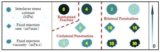
Figure 12. Impact of the stress contrast and fracturing fluid parameters on fracture penetration.

4. Conclusions

A model of HF propagation through sandstone–shale interbeds is built using XSite software. Some interesting findings are as follows:

(1)

The higher the tensile strength and the greater the type-I fracture toughness of the shale layer, the more pronounced the inhibitory effect on the propagation of HFs. The smaller the interlayer stress contrast, the higher the fracturing fluid flow rate, and the greater the fracturing fluid viscosity, the easier it is for the HF to vertically penetrate the rock interface.

(2)

The propagation of HFs is inversely correlated with shale fracture toughness, tensile strength, and Poisson’s ratio, and directly correlated with elastic modulus. The larger the Poisson’s ratio and the smaller the elastic modulus of the shale layer, the greater the rock fracture toughness and tensile strength, ultimately resulting in a smaller HF.

(3)

When the effect of lithological interfaces is considered, an increasing interlayer stress contrast causes the HF to gradually transition from penetrating the interfaces to becoming confined between the two interfaces. When the influence of the lithological interface is not considered, the shape of the HF gradually transforms from a penny-shaped fracture to a blade-shaped fracture.

References

- Tan, P.; Jin, Y.; Hou, B.; Zheng, X.; Guo, X.; Gao, J. Experiments and analysis on hydraulic sand fracturing by an improved true tri-axial cell. J. Petrol. Sci. Eng. 2017, 158, 766–774. [Google Scholar] [CrossRef]
- Liao, S.Z.; Hu, J.H.; Zhang, Y. Mechanism of hydraulic fracture vertical propagation in deep shale formation based on elastic–plastic model. Eng. Fract. Mech. 2024, 295, 109806. [Google Scholar] [CrossRef]
- Yang, X.F.; Chang, C.; Cheng, Q.Y.; Xie, W.; Hu, H.; Li, Y.; Huang, Y.; Peng, Y. The influence of rock and natural weak plane properties on the vertical propagation of hydraulic fractures. Processes 2024, 12, 2477. [Google Scholar] [CrossRef]
- Wang, Y.Z. Mechanism and Engineering Application of Vertical Penetration Fracturing in Terrestrial Shale Oil Reservoirs. Ph.D. Thesis, China University of Petroleum, Beijing, China, 2023. [Google Scholar] [CrossRef]
- Zhang, T.J. Study on Fracture Propagation Law of Hydraulic Fracturing in Bedding Formation. Master’s Thesis, Shijiazhuang Tiedao University, Shijiazhuang, China, 2024. [Google Scholar] [CrossRef]
- Li, J.L.; Zhong, Y.; Yan, Y.H.; Huang, T.; Mou, Q.; Yang, B. Mechanism of hydraulic fracture propagation and the uneven propagation behavior of multiple clusters in shale oil reservoirs. Fuel 2025, 395, 135241. [Google Scholar] [CrossRef]
- Lu, Y.R.; Cai, Z.; Huang, D.; Yao, X.; Ma, Q.; Chen, D. Peridynamic modeling and analysis of interfacial crack propagation by hydraulic fracturing in layered shale. Comput. Geotech. 2025, 184, 107280. [Google Scholar] [CrossRef]
- Zhao, Y.X.; Wang, L.; Ma, K.; Zhang, F. Numerical simulation of hydraulic fracturing and penetration law in continental shale reservoirs. Processes 2022, 10, 2364. [Google Scholar] [CrossRef]
- Ju, Y.; Liu, P.; Chen, J.L.; Yang, Y.; Ranjith, P.G. CDEM-based analysis of the 3D initiation and propagation of hydrofracturing cracks in heterogeneous glutenites. Nat. Gas. Sci. Eng. 2016, 35, 614–623. [Google Scholar] [CrossRef]
- Zheng, H.; Li, F.X.; Wang, D. Numerical Investigation of Complex Hydraulic Fracture Propagation in Shale Formation. Processes 2024, 12, 2630. [Google Scholar] [CrossRef]
- Fu, S.H.; Hou, B.; Xia, Y.; Chen, M.; Wang, S.; Tan, P. The study of hydraulic fracture height growth in coal measure shale strata with complex geologic characteristics. J. Petrol. Sci. Eng. 2022, 211, 110164. [Google Scholar] [CrossRef]
- Gao, Y.; Qin, Q.P.; Bian, X.B.; Wang, X.; Xu, W.; Zhao, Y. Propagation law of hydraulic fractures in continental shale reservoirs with sandstone–shale interaction. Processes 2024, 12, 2931. [Google Scholar] [CrossRef]
- Tang, J.Z.; Wu, K.; Zeng, B.; Huang, H.; Hu, X.; Guo, X.; Zuo, L. Investigate effects of weak bedding interfaces on fracture geometry in unconventional reservoirs. J. Petrol. Sci. Eng. 2018, 165, 992–1009. [Google Scholar] [CrossRef]
- Ma, P.C.; Tang, S.F. Simulation of key influencing factors of hydraulic fracturing fracture Propagation in a shale reservoir based on the displacement discontinuity method. Processes 2024, 12, 1000. [Google Scholar] [CrossRef]
- Hou, Z.K.; Cheng, H.L.; Sun, S.W.; Chen, J.; Qi, D.Q.; Liu, Z.B. Crack propagation and hydraulic fracturing in different lithologies. Appl. Geophys. 2019, 16, 243–251. [Google Scholar] [CrossRef]
- Yang, L.Z.; Wang, X.Y.; Niu, T. Propagation characteristics of multi-cluster hydraulic fracturing in shale reservoirs with natural fractures. Appl. Sci. 2025, 15, 4418. [Google Scholar] [CrossRef]
- Zhuo, R.Y.; Ma, X.F.; Li, J.M.; Zhang, S.; Zou, Y.; Ma, J. Study on the effect of fluid viscosity and injection rate on the geometry of hydraulic fractures penetrating through laminae planes and the proppant distribution in deep shale oil reservoirs. Rock Mech. Rock. Eng. 2024, 58, 2763–2780. [Google Scholar] [CrossRef]
- Khormali, A.; Ahmadi, S.; Aleksandrov, N.A. Analysis of reservoir rock permeability changes due to solid precipitation during waterflooding using artificial neural network. J. Pet. Explor. Prod. Technol. 2025, 15, 17. [Google Scholar] [CrossRef]
- Huang, L.K.; Liu, J.J.; Zhang, F.S.; Fu, H.; Zhu, H.; Damjanac, B. 3D lattice modeling of hydraulic fracture initiation and near-wellbore propagation for different perforation models. J. Petrol. Sci. Eng. 2020, 191, 107169. [Google Scholar] [CrossRef]
- Huang, B.X.; Liu, J.W. Experimental investigation of the effect of bedding planes on hydraulic fracturing under true triaxial stress. Rock Mech. Rock. Eng. 2017, 50, 2627–2643. [Google Scholar] [CrossRef]
- Whittaker, B.N.; Singh, R.N.; Sun, G. Rock Fracture Mechanics: Principles, Design and Applications; Elsevier: Amsterdam, The Netherlands, 1992; ISBN 0444896848. [Google Scholar]
- Deng, H.F.; Zhu, M.; Li, J.L.; Wang, Y. Study of mode-I fracture toughness and its correlation with strength parameters of sandstone. Rock. And. Soil Mech. 2012, 33, 3585–3591. [Google Scholar] [CrossRef]
Disclaimer/Publisher’s Note: The statements, opinions and data contained in all publications are solely those of the individual author(s) and contributor(s) and not of MDPI and/or the editor(s). MDPI and/or the editor(s) disclaim responsibility for any injury to people or property resulting from any ideas, methods, instructions or products referred to in the content. |
© 2025 by the authors. Licensee MDPI, Basel, Switzerland. This article is an open access article distributed under the terms and conditions of the Creative Commons Attribution (CC BY) license (https://creativecommons.org/licenses/by/4.0/).