Multiphysics Numerical Simulation Model and Hydraulic Model Experiments in the Argon-Stirred Ladle

Abstract

The argon-stirred ladle is a standard piece of steelmaking refining equipment. The molten steel quality will improve when a good argon-stirred process is applied. In this paper, a Multiphysics model that contained fluid flow, bubble transport, alloy transport, bubble heat flux, alloy heat flux, alloy melting, and an alloy concentration species transport model was established. The fluid model and bubble transport model that were used to calculate the fluid velocity were verified by the hydraulic model of the ladle that was combined with particle image velocimetry measurement results. The numerical simulation results of the temperature fields and steel–slag interface shape were verified by a ladle that contained 25 t of molten steel in a steel plant. The velocity difference between the hydraulic model and numerical model decreased when the C_L (integral time-scale constant) increased from 0 to 0.3; then, the difference increased when the C_L increased from 0.3 to 0.45. The results showed that a C_L of 0.3 approached the experiment results more. The bubble heat flux model was examined by the industrial practice, and the temperature decrease rate was 0.0144 K/s. The simulation results of the temperature decrease rate increased when the initial bubble temperature decreased. When the initial bubble temperature was 800 °C, the numerical simulation results showed that the temperature decrease rate was 0.0147 K/s, and the initial bubble temperature set at 800 °C was more appropriate. The average melting time of the alloy was 12.49 s and 12.71 s, and the mixture time was approximately the same when the alloy was added to two slag eyes individually. The alloy concentration had fewer changes after the alloy was added in the ladle after 100 s.

1. Introduction

In metallurgy, the argon-stirred ladle is a low-cost, highly efficient, and common refining method for the improvement of the molten steel temperature, the homogeneity ofmolten steel concentration [1,2,3,4,5,6,7,8,9], inclusion floatation [10,11,12,13,14,15,16], and increase in the kinetic reaction [17,18,19,20] in the ladle.

Studies on the argon-stirred ladle numerical simulation have focused on the following topics: (1) fluid-flow simulation [21], (2) bubble transport modeling, (3) temperature simulation, (4) alloy melting, (5) alloy concentration or other species transport [22], and (6) kinetic reaction in the ladle. In the fluid-flow simulation, the Euler–Euler approach [23,24], the single-phase methods by exerting an additional force on the fluid flow [25,26,27], the multiphase volume of fluid (VOF) method [2,28,29,30], and the Euler–Lagrange method [31,32,33] considered the bubble as a discrete phase and the molten steel and molten slag as the continuum phase. In the bubble transport modeling, Xue et al. [34] studied the effect of small bubbles on inclusion removal, and the results showed that the small bubble is beneficial to inclusion removal. Zhu et al. [35] studied the effect of an argon-stirred ladle on the inclusion removal, and the results showed that a larger size of inclusion will be removed more quickly and the difficulty of the inclusion removal will increase when the inclusion diameter decreases. In the molten steel temperature simulation, Urióstegui-Hernández [36] considered the heat transfer between the fluid and the bubble using the Euler–Euler methods. Cheng et al. [37] studied the effect of the slot plug on the flow in the ladle and temperature exchange with the argon. In the alloy melting simulation, Bhattacharjee et al. [38] studied the alloy melting in the argon-stirred ladle by numerical simulation, and the results showed that dissolution rates are a function of gas flow rate and vessel dimensions and depend on the diffusivity of the alloy and initial size. In the alloy concentration or other species, Liu et al. [28] studied the species transport in the argon-stirred ladle, and monitoring the species concentration varies with solution time. In the kinetic reaction in the ladle studies, Kwon et al. [39] studied the Al-deoxidation in the argon-stirred ladle to predict the inclusion formation. Lachmund et al. [40] established a desulfurization model and predicted the desulphurization process by numerical simulation. Singh et al. [41] studied the desulfurization with kinetic data acquired from Thermo-Calc software, and the results showed that dual plugs are better than a single plug when the flow is the same.

Recently, Mantripragada [36] studied the argon plugs’ position and flow rate on the argon-stirred ladle refined by numerical simulation. They pointed out a dimensional variation in the optimized ladle. Wondrak et al. [42] used Sn-Bi alloy in industrial experiments, and the results showed the ‘slag eye’ size and velocity magnitude in the molten alloy surface. The experimental results will benefit the numerical simulation optimization. Uriostegui-Hernandez et al. [43] studied the fluid flow and mass transfer of sulfur; the results showed that the desulfurization rates increase as the argon gas flow rate increases. Wang et al. [44] studied the effect of the argon-stirred process on the ladle refractory erosion by numerical simulation and industrial practice. The results showed that the refractory erosion will increase near the slag layer and near the bottom gas inlet. Joubert [45] studied the mass transfer of the species in the steel–slag phase in the argon-stirred ladle by a numerical simulation and a hydraulic model simulation. The results showed that the numerical simulation model of species transport showed good consistency with the hydraulic simulation. Guo et al. [16] studied the effect of plug position, argon flow rate, and inclusion size on the inclusion removal. The results showed that the inclusion removal rate will increase when the argon flow rate grows. Riabov et al. [46] studied the bubble diameter, plume area, and bubble velocity using a hydraulic model combined with particle image velocimetry technology. The results showed that the increase in the diameter of the porous plug will lead to a small bubble diameter and poorer mixing conditions. Li et al. [47] studied the bubble transport and fluid flow in an argon-stirred ladle by the volume of the fluid (VOF) model with a finer scale of mesh coupling with a sub-grid-scale large eddy simulation. The results showed that the slag eye size varies with time, and the bubble detachment frequency has a direct effect on the slag eyes. A new correlation of the slag eye and the modified Froude number was established.

In the previous work, the argon-stirred ladle that contained molten steel was 80~300 t. The tundish was applied in the argon-stirred ladle during the casting process. The tundish is helpful in the molten steel temperature, species homogeneity, and inclusion removal. However, there is no tundish in the casting process; when the argon-stirred steel that contained molten steel is about 25~30 t, the effect of molten steel temperature, species homogeneity, and fluid flow in the argon-stirred ladle is essential. In this paper, a numerical simulation model was established that contained a fluid flow simulation, bubble transport, alloy transport, alloy melting, alloy concentration species transport, and a bubble and alloy heat transfer simulation. In this paper, a random walk model was introduced to simulate the bubble transport and bubble drive flow novelty. The effect of random transport parameters on the bubble drive flow simulation was examined by particle image velocimetry results of the hydraulic model. The heat transfer model of the bubble and the molten steel was introduced for the first time, and the bubble heat transfer simulation was examined by industrial practice where the ladle contained 25 t of molten steel in a steel plant. The molten steel temperature distribution in the ladle was revealed for the first time. The effect of the alloy-added situation on the alloy concentration diffusion was discussed. The numerical simulation model was helpful in the argon-stirred ladle design and process modification.

2. Experimental Methods

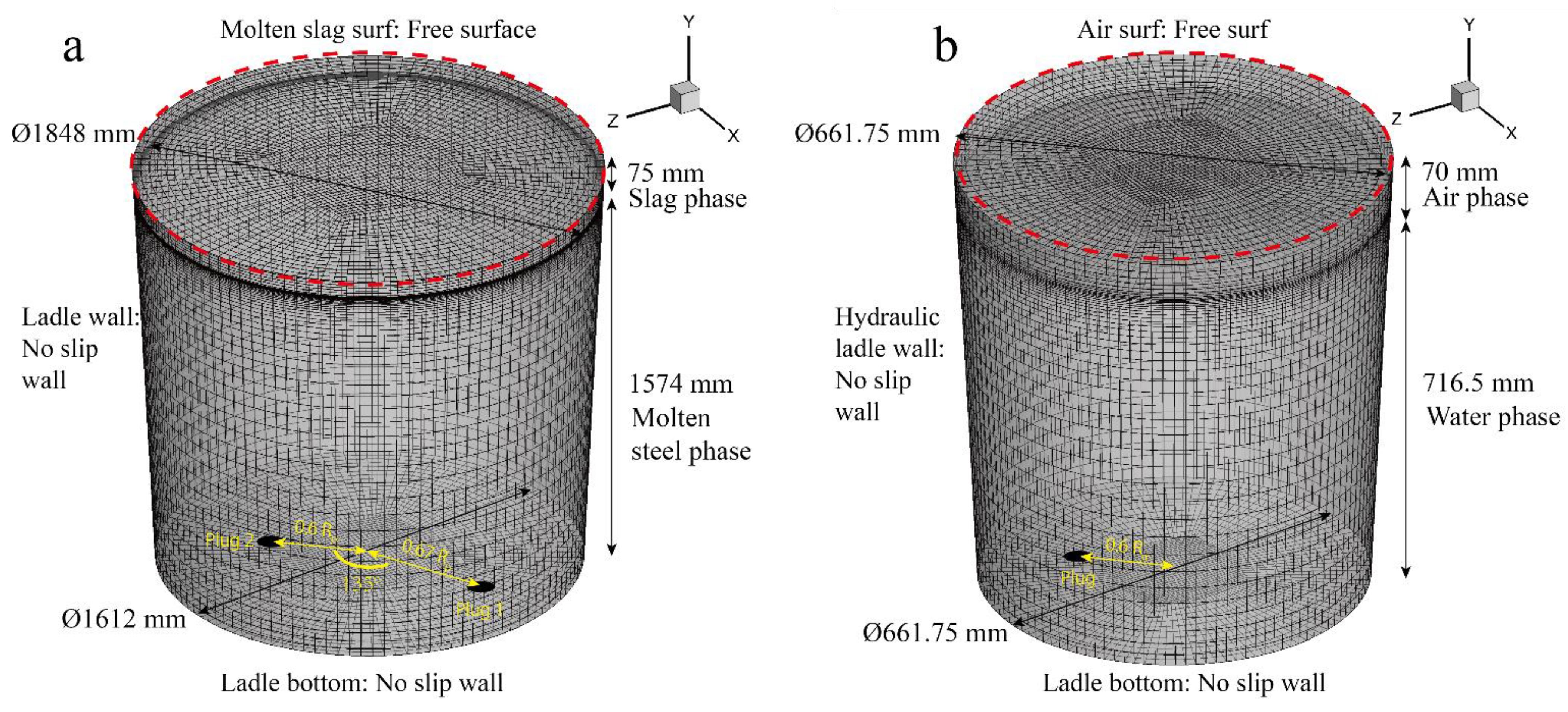
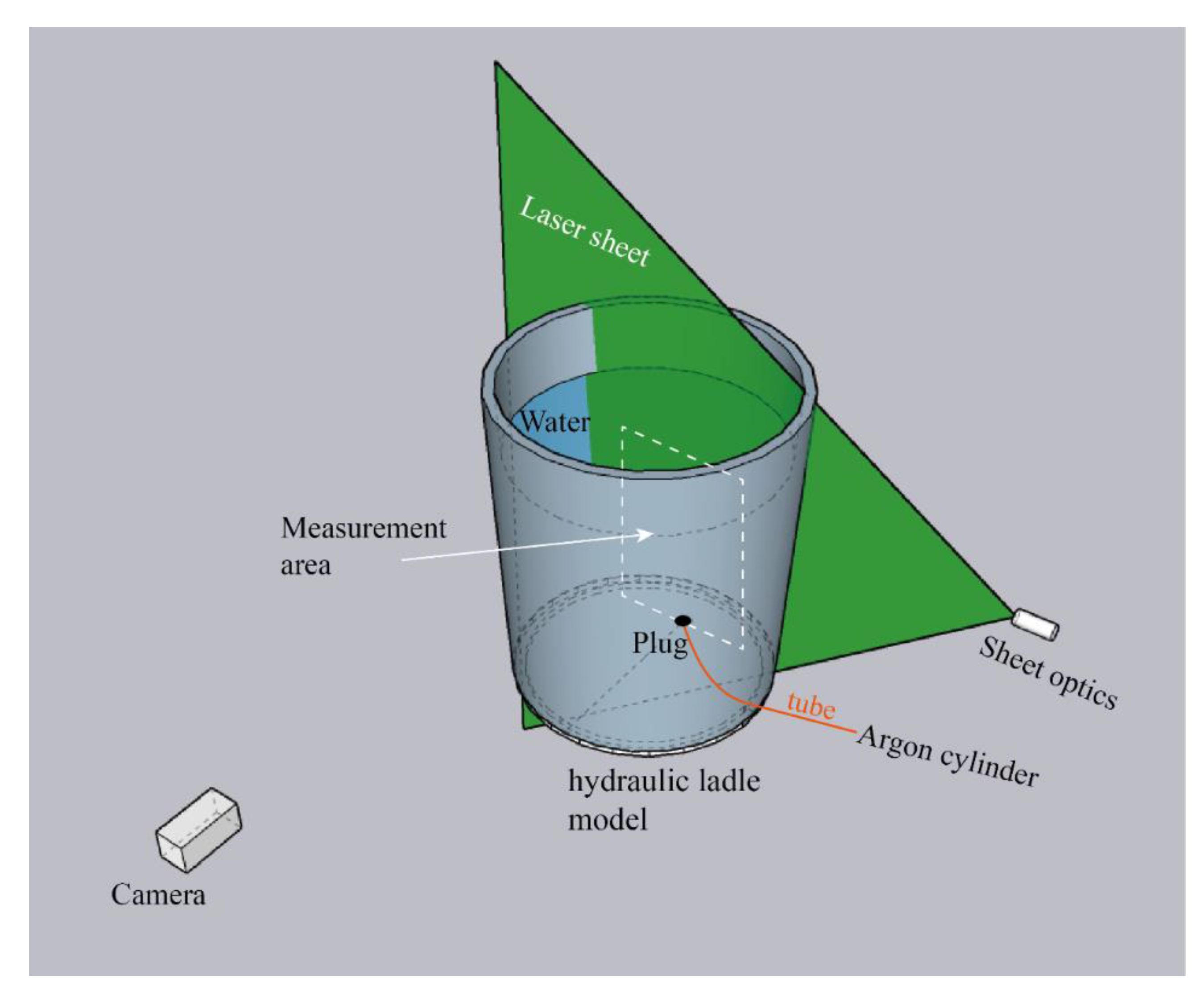
2.1. The measurement of the Fluid Flow in the Ladle Water Model

A hydraulic model of the ladle was established by the principle of hydraulic similarity. The ratio was 1:2.4 between the water model and the prototype. The dimensions of the argon-stirred ladle in the prototype and water model are shown in

Table 1. The dimensions of argon-stirred ladle in prototype and water model.

Item	Parameters
The bottom diameter of the hydraulic model/mm	661.75
Top diameter of the hydraulic model/mm	752
Height of the hydraulic model/mm	910.5
Height of water/mm	716.5
Position of argon plug in the hydraulic model	0.6 Rm
The bottom diameter of the prototype ladle/mm	1612
Top diameter of prototype ladle/mm	1848
Height of the prototype ladle/mm	2374
Hight of molten steel/mm	1574
Position of argon plugs in prototype	0.6 Rp and 0.67 Rp

Where R represents the radius, subscript m represents the hydraulic model, and p represents the prototype.

. The angle between the two plugs was 135° in the prototype. The fluid velocity in the hydraulic model was measured by particle image velocimetry (PIV) technology. The prototype ladle can contain 25 t of molten steel.

Figure 1 shows the schematic of the velocity measurements in the hydraulic ladle. The plug was placed at 0.6R_m, and the laser sheet emission was from the right side and passed through the plug. The camera was vertical to the plane where the laser sheet was at. The flow rate was 6 L·min⁻¹, controlled by the valve, and the argon flowed through the tube and out from the plug. The PIV equipment contained: laser (Litron lasers LPY704-100 PIV, Rugby, UK), guiding arm (LaVision Gmbh, Göttingen, Germany), sheet optics, Nikon AF-S 50 mm f/1.4 G lens (Nikon Corporation, Tokyo, Japan), calibration plate (LaVision Gmbh, Germany), camera (LaVision Gmbh, Germany), programmable timing unit X (PTU X), workstation (Intel(R), Xeon(R), CPU E5-2650 v3 @ 2.30 GHz, two processors), laser power equipment, and laser cooling equipment. The measurement and postprocessing were accomplished by the DaVis 8.4.0 (LaVision GmbH, Germany). The seeding particle was vestosint and the seeding particle diameter was 55 μm; it had a good flow following. The laser shutter opened twice in a very short time, and the camera exposed twice following the laser shutter opening. The time interval of the laser shutter opening twice was 0.01428 s, the camera acquisition rate was 70 Hz, and the acquisition time lasted two seconds. During the measurement, the sampling count was 100 and the time-averaged results were calculated by DaVis 8.4.0. The postprocessing was a cross-correlation model, the interrogation window size was 96 × 96 window size, and the interrogation window was decreased to 64 × 64 window size.

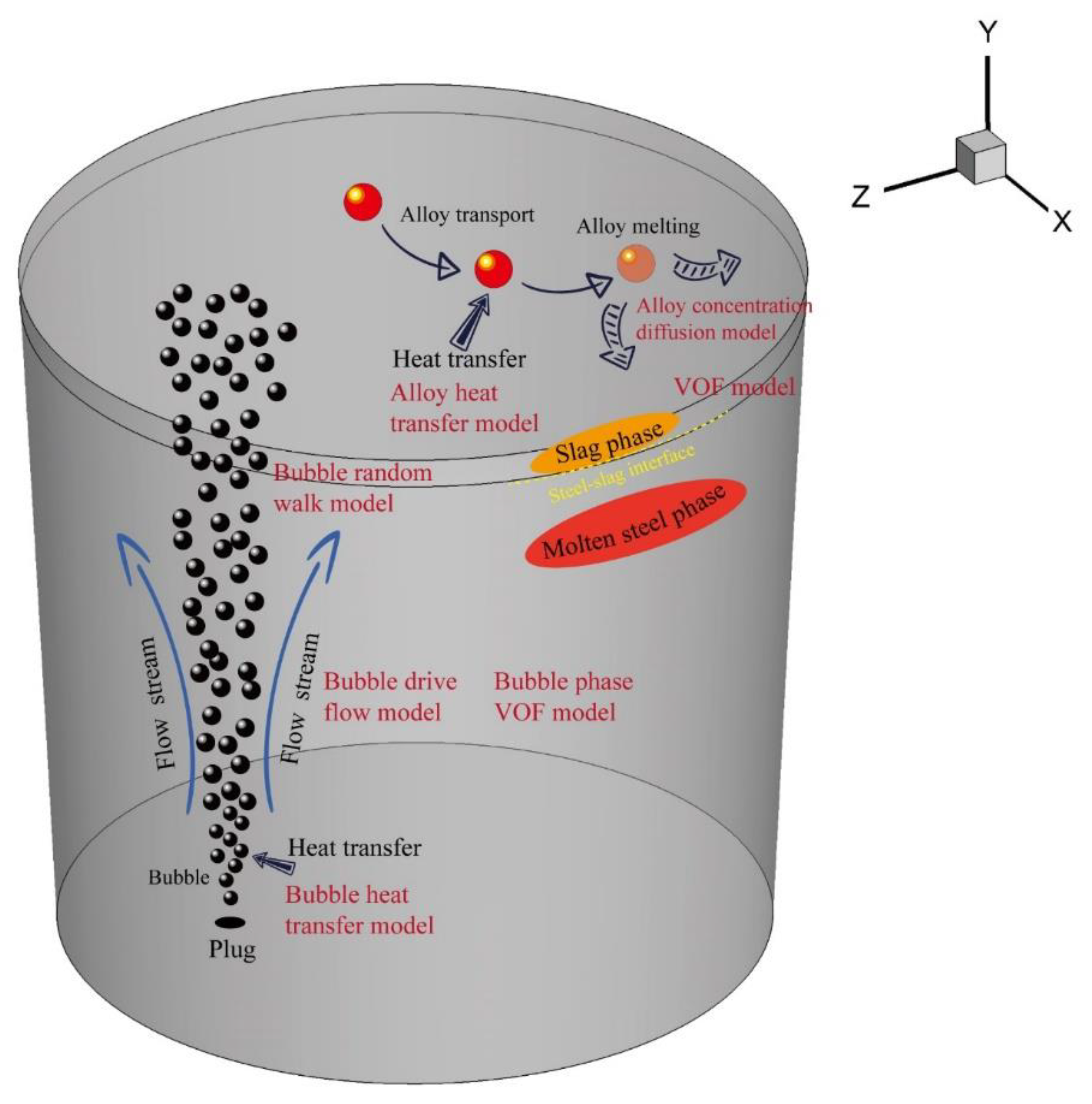
2.2. Numerical Simulation Models

Figure 2 shows the schematic of the numerical simulation model included in the paper. The numerical simulation model had the following part: the fluid flow model, the bubble and alloy transport model, the bubble and fluid heat exchange model, the alloy melting model, the VOF model, and the alloy concentration diffusion model.

2.2.1. Fluid Flow and VOF Model

In this paper, the fluid flow was driven by bubble transport. The governing equations are shown in Equations (1)–(7), and a source term was added to simulate the flow driven by the bubble. The drag force was considered in this paper as the bubble-driven flow, and the source term was added. In this paper, three kinds of fluid phases were considered: molten steel phase, molten slag phase, and argon bubble phase. The continuum surface stress and surface tension models were used in the VOF model. The volume fraction of the bubble in the fluid domain was adjusted by the User-Defined Function (UDF) module. The volume fraction of the bubble was updated according to the bubble’s position.

$$\frac{1}{{\rho }_q}\frac{\partial }{\partial t}({\alpha }_q{\rho }_q)+\nabla \cdot ({\alpha }_q{\rho }_q\overrightarrow{v})=0$$

(1)

$${\displaystyle \sum _{q=1}^n{\alpha }_q=1}$$

(2)

$$\frac{\partial }{\partial t}(\rho \overrightarrow{v})+\nabla (\rho \overrightarrow{v}\overrightarrow{v})=-\nabla p+\nabla (\mu (\nabla \overrightarrow{v}+\nabla {\overrightarrow{v}}^{\mathrm{T}})-\frac{2}{3}\nabla \overrightarrow{v}I)+\rho \overrightarrow{g}+\overrightarrow{F}$$

(3)

$$\frac{\partial }{\partial t}(\rho k)+\frac{\partial }{\partial x_i}(\rho k{u}_i)=\frac{\partial }{\partial x_j}({\alpha }_k{\mu }_{eff}\frac{\partial k}{\partial x_j})+G_k+G_b-\rho \epsilon$$

(4)

$$\frac{\partial }{\partial t}(\rho \epsilon )+\frac{\partial }{\partial x_i}(\rho \epsilon u_i)=\frac{\partial }{\partial x_j}({\alpha }_{\epsilon }{\mu }_{eff}\frac{\partial \epsilon }{\partial x_j})+C_{1\mathsf{\epsilon }}\frac{\epsilon }{k}(G_k+C_{2\mathsf{\epsilon }}{G}_b)+C_{2\mathsf{\epsilon }}\rho \frac{{\epsilon }^2}{k}-R_{\mathsf{\epsilon }}+S_{\epsilon }$$

(5)

$$\overrightarrow{F}=\frac{{\alpha }_l}{\Delta V_{\mathrm{cell}}}{\displaystyle \sum _i^N({\overrightarrow{F}}_{D,i})}Q△t$$

(6)

$${\overrightarrow{F}}_{D,i}=\frac{18\mu C_{D,i}{\mathrm{Re}}_i}{24d_{b,i}^2{\rho }_{b,i}}({\overrightarrow{u}}_l-{\overrightarrow{u}}_{b,i})$$

(7)

where α_q represents the volume fraction of the qth phase, ρ_q represents the density in the qth phase, v represents the velocity, n represents the phase count in the simulation, ρ represents the density, μ represents the molecular viscosity, I is the unit tensor, $\overrightarrow{F}$ is the source term of the bubble-driven flow, k represents the turbulent kinetic energy, G_k represents the generation of turbulence kinetic energy due to the mean velocity gradient, G_b is the generation of turbulence kinetic energy due to buoyancy, ε is turbulent kinetic energy dissipation, α_l represents the volume fraction of the liquid phase, ΔV_cell represents the volume of the cell, N represents the bubble count in the cell, Q represents the flow rate of the argon, Δt represents the time step, C_D,i represents the coefficient of drag force, Rei represents the Reynolds number of bubble, d_b,i represents the diameter of the bubble, ρ_b,i represents the density of the bubble, u_l is the velocity of the fluid, and u_b,i is the velocity of the bubble.

2.2.2. Bubble and Alloy Transport Model

The discrete phase model (DPM) was applied in the bubble and inclusion transport modeling. The bubble and alloy transport equations are shown in Equations (8)–(10). The discrete random walk model was applied in the bubble transport simulation. The randomness of the inclusion transport will increase if the C_L is increased. The bubble will be removed when the bubble reaches the steel–slag interface. The steel–slag interface is when the volume fraction of slag is 0.5. The bubble diameter will increase if the bubble floats. The bubble diameter variation mechanism is shown in Equation (11).

$$\frac{d{\overrightarrow{u}}_p}{dt}=\frac{{\overrightarrow{u}}_l-{\overrightarrow{u}}_p}{{\tau }_r}+\frac{\overrightarrow{g}({\rho }_p-{\rho }_{\mathrm{f}})}{{\rho }_p}$$

(8)

$$T_E=-T_L\ln (r)$$

(9)

$$T_L=C_L\frac{k}{\epsilon }$$

(10)

$$d_{b,i}=\sqrt[3]{\frac{p_0+{\rho }_{\mathrm{l}}gh}{p_0+{\rho }_{\mathrm{l}}g(H-y_i)}}{d}_{\mathrm{bottom}}$$

(11)

where $\overrightarrow{u_p}$ and ${\overrightarrow{u}}_l$ are, respectively, the particle vector and the fluid vector; ρ_p is the particle density; ρ_f is the fluid density; T_E is the eddy lifetime; r is the random Gaussian number; T_L is the integral time scale; C_L (integral time-scale constant) is a constant.

2.2.3. Energy Conservation and Bubble Heat Exchange Model

The governing equation of the temperature is shown in Equations (12) and (13). In this paper, a heat transport model of molten steel and the bubble was applied. The equations of the bubble heat transport are shown in Equations (14)–(19). The bubble temperature is lower than the molten steel temperature, and the heat will transfer from the molten steel to the bubble. The heat transfer energy is based on the energy conservation law. The bubble will stop heat transfer if the bubble temperature is the same as that of the molten steel. The effect of bubble initial injection temperature on the molten steel temperature simulation is discussed in Section 3.2.2.

$$\frac{\partial }{\partial t}(\rho E)+\nabla (\overrightarrow{v}(\rho E+p))=\nabla (k_{eff}\nabla T-{\displaystyle \sum _j{h}_j{\overrightarrow{J}}_j}+({\overline{\overline{\tau }}}_{eff}\cdot \overrightarrow{v}))$$

(12)

$$E=h-\frac{p}{\rho }+\frac{v^2}{2}$$

(13)

$$E_T=C_{b,i}\cdot m_{b,i}\cdot (T_{\mathrm{cell}}-T_{b,init})$$

(14)

$$E_{step}=Nu\cdot k_m\cdot \pi \cdot d_{\mathrm{b},\mathrm{i}}\cdot (T_{\mathrm{cell}}-T_{b,pre.temp})\cdot △t$$

(15)

$$Nu=2+0.6\cdot {\mathrm{Re}}^{1/2}\cdot {\mathrm{Pr}}^{1/3}$$

(16)

$$T_{b,cur.temp}=T_{b,pre.temp}+\frac{E_{step}}{(C_{b,i}\cdot m_{b,i})}$$

(17)

$$\mathrm{Pr}=\frac{{\mu }_f\cdot C_p}{k_m}$$

(18)

$${\mathrm{Re}}_{\mathrm{p}}=\frac{{\rho }_{b,i}{d}_{b,i}({\overrightarrow{u}}_l-{\overrightarrow{u}}_{b,i})}{{\mu }_l}$$

(19)

where h is sensible enthalpy, E_T is the total energy of the bubble, C_b.i is the heat capacity of the bubble, m_b.i is the bubble mass, T_cell is the cell’s temperature where the bubble is injected into the fluid domain, T_b.init is the initial bubble temperature, E_step is the energy exchange in each timestep, Nu is the Nusselt number, k_m is the fluid thermal conductivity, T_{b, pre.temp} is the bubble temperature in the previous timestep, and C_p is the heat capacity of the fluid.

2.2.4. Alloy Melting and Alloy Concentration Diffusion Model

In this paper, a solid crust will form when the alloy is added to the high-temperature molten steel. At this time, the alloy began melting inside the solid crust. The alloy concentration was released until the solid crust melted at a specific time. The alloy concentration numerical simulation governing equation is shown in Equations (20)–(24). The source term was added in a cell where the alloy melted.

$$t_{melt}=\frac{{\rho }_A{C}_{P,A}{d}_A}{2\pi h_{\mathrm{c}}}\frac{T_s-T_0}{T_M-T_s}$$

(20)

$$Nu=\frac{d_A{h}_{\mathrm{c}}}{k_m}$$

(21)

$$Nu=2+(0.4{\mathrm{Re}}_A{}^{1/2}+0.06{\mathrm{Re}}_A{}^{2/3})\cdot {\mathrm{Pr}}^{2/5}$$

(22)

$$\frac{\partial \rho C}{\partial t}+\frac{\partial }{\partial x_i}(\rho u_{i}C-{\Gamma }_k\frac{\partial C}{\partial x_i})=S_C$$

(23)

$$S_C=\frac{m_{alloy}}{m_{\mathrm{cell}}}$$

(24)

where t_melt is the alloy solid crust melting time, ρ_A is the alloy density, C_P,A is the heat capacity of the alloy, d_A is the diameter of the alloy, h_c is the coefficient of the heat transfer, T_s is the solidification temperature of molten steel, T_M is the temperature of molten steel, T₀ is the initial alloy temperature, C is the mass concentration of alloy, S_c is the source term of the alloy melting, m_alloy is the mass of the melted alloy, and m_cell is the mass of the cell where the alloy is melting.

2.3. Boundary Condition and Solution Strategy

Table 2. Relevant parameters in the numerical simulation.

Item	Parameters
Water density (25 °C)/kg·m−3	997.04
Water viscosity (25 °C)/Pa·s	0.8949 × 10−3
Air phase density (25 °C)/kg·m−3	1.185
Air phase viscosity (25 °C)/Pa·s	1.8315 × 10−5
Water surface tension/N·m−1	0.07197
Argon bubble flow rate in hydraulic model/L·min−1	6
Molten steel density/kg·m−3	7000
Molten steel viscosity/Pa·s	0.0067
Molten slag density/kg·m−3	3500
Molten slag viscosity/Pa·s	0.06
Argon density/kg·m−3	1.784
Argon viscosity/Pa·s	2.2624 × 10−5
Molten steel–slag interface surface tension/N·m−1	1.6
Molten steel specific heat/J·kg−1·K−1	680
Molten slag specific heat/J·kg−1·K−1	1100
Argon specific heat/J·kg−1·K−1	1006.43
Molten steel thermal conductivity/W·m−1·K−1	40.3
Molten slag thermal conductivity/W·m−1·K−1	34
Argon thermal conductivity/W·m−1·K−1	0.0242
Alloy density/kg·m−3	5780
Alloy specific heat/J·kg−1·K−1	364
Alloy diameter/mm	50
Alloy thermal conductivity/W·m−1·K−1	26.32
Initial alloy temperature/°C	25
Initial bubble temperature/°C	25, 400, 800
Alloy concentration diffusion coefficient/m2·s−1	1.566 × 10−14
Argon bubble flow rate in prototype/L·min−1	5

shows the relevant parameters that are required in the numerical simulation. The initial bubble diameter and the initial bubble velocity were calculated by Equations (23) and (24). The numerical simulation was calculated by ANSYS Fluent software (ANSYS, Inc., Canonsburg, PA, USA). The inlet boundary condition was set as follows: the bubbles were injected from the plugs, and the inject position was defined by the User-Defined Function (UDF) that was built in the ANSYS Fluent software (ANSYS, Inc., Canonsburg, PA, USA). The boundary name, position, and condition are shown in Figure 3. The bubble flow rate was 5 L·min⁻¹. The bubble injection velocity was 2.63 m·s⁻¹ in this paper. The initial bubble diameter was 3.924 mm. The position of the alloys thrown was above the slag eye by 2.5 m; based on the law of free fall, the velocity of the alloy contacting with the molten steel was 7 m·s⁻¹. Figure 3 shows the hexahedral mesh of the fluid zone in the prototype and hydraulic model. The argon bubble was injected from the bottom of the ladle, and the injection position is shown in Figure 3. In the prototype, argon was injected at two places, and the angle between them was 135°. The solution initialization used standard initialization and computing from all zones. The solution step was 0.001 s, the injection rate of the bubble was one bubble per solution step, and the N_per was 1000. The free surface was used on the top of the slag (in prototype modeling) or the top of the air (in the hydraulic modeling). The rest boundary was taken as the wall boundary. The SIMPLE scheme was used in the pressure-velocity coupling. The residual in the governing equations was 0.001. The heat flux in the ladle wall, the molten slag surf, and the ladle bottom was 0.006 W²·mm⁻².

$$d_{b,init}=(0.35\cdot {(\frac{Q^2}{9.8})}^{0.2})$$

(25)

$$v_{b.init}=\frac{Q}{(N_{per}\cdot \frac{1}{6}\cdot \pi \cdot d_{b,init}^3)}$$

(26)

where v_b,init is the initial velocity when the bubble is injected into the fluid zone and N_per is the bubble injection count in 1 s.

3. Results and Discussion

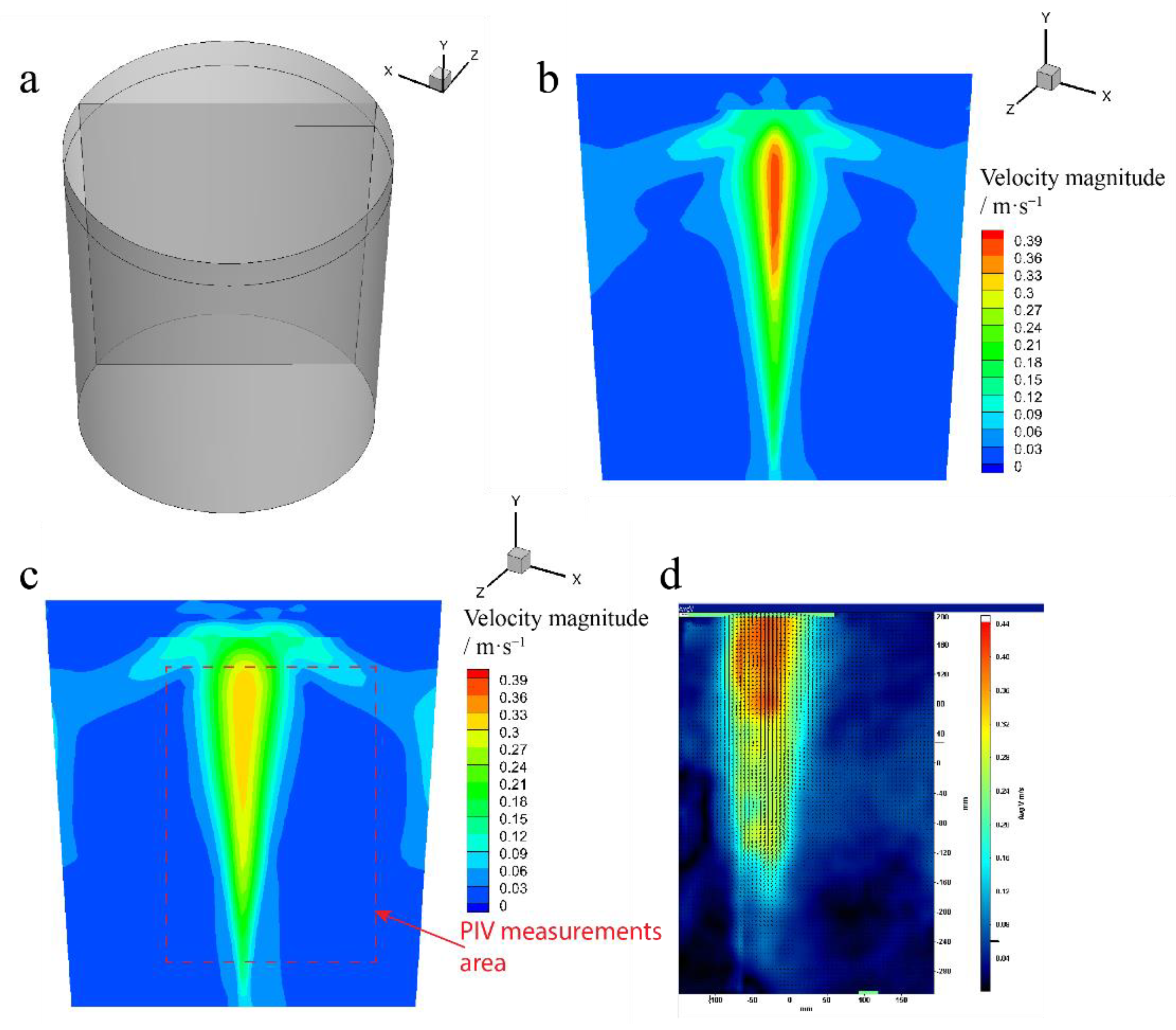
3.1. Model Validation

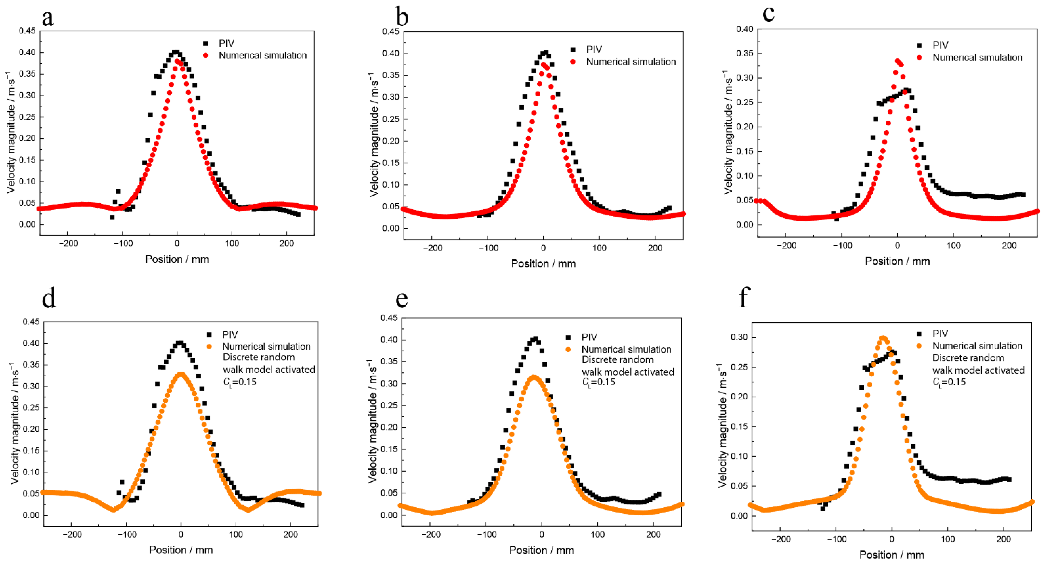
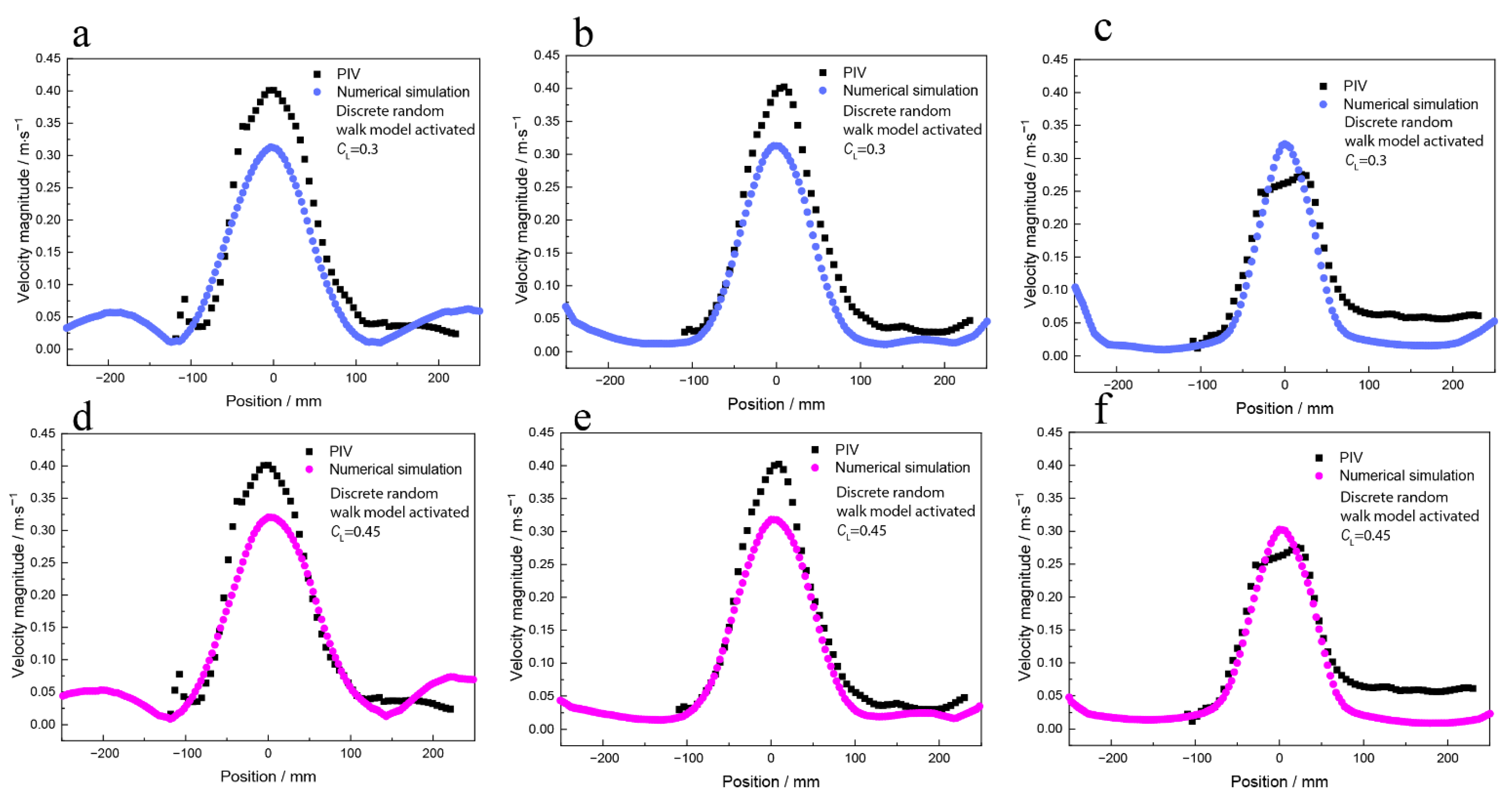
3.1.1. Effect of Discrete Random walk Model on the Simulation Results

Figure 4 shows the simulation results of the water model simulation and the PIV measurements results of the water model. Figure 4a shows the slice position of the numerical simulation results. The PIV measurements area is identical to the slice position. Figure 4b shows the velocity contour of the slice position, the velocity is higher in the center, and the bubbles are transported in the center, which accelerates the fluid velocity when the bubble random transport model is deactivated. The bubble is upward in a straight line, and the velocity contour is symmetrical. Figure 4c shows the velocity contour when the bubble random transport model is activated, and the C_L is 0.15. The area of the velocity at a higher speed is in a reverse cone shape. The maximum velocity is lower than when the random walk model is deactivated. The bubbles are transported in a random way; the degree of dispersion of the bubble position is higher, which results in a lower maximum velocity. Figure 4d shows the PIV measurement result, and the measurement area is plotted in Figure 4c in a red scatter line. Figure 4d shows that the velocity is higher at the top of the ladle model, the velocity in a higher-speed area is in a reverse cone shape, and the velocity contour distribution of the numerical simulation is similar to the PIV measurement results.

Figure 5 shows the quantitative data of the velocity magnitude of the numerical simulation and PIV measurement results. Figure 5a–c show the simulation results of the bubble random walk model being deactivated and the PIV measurement results. The results show that the velocity magnitude distribution is sharp, and the velocity peak is narrow and higher compared to the PIV results. The flow of the fluid in the water model is driven by the bubbles. When the bubble random walk model is deactivated, the flow of the bubbles in the fluid presents a vertical upward movement, so the velocity peaks appear high and narrow. Figure 5d–f show the simulation results when the bubble random walk model is activated, the C_L is 0.15, and the PIV measurements results. The velocity magnitude peak is smaller and broader than when the bubble random walk model is deactivated.

3.1.2. Effect of Time Scale Factor on the Simulation Results

Figure 6 shows the velocity magnitude of the numerical simulation results and the PIV measurements. The numerical simulation result under the case of C_L is 0.3 or 0.45. Figure 7 shows the variance in the velocity difference between the numerical simulation and the PIV measurement results. The calculation range is the velocity data from −100 mm to 100 mm.

In Figure 7, D_L represents the variance in the velocity magnitude difference between the numerical simulation and the PIV measurements, where a C_L of 0 illustrates the case where the bubble random transport model is deactivated. The results show that the variance is decreased when the C_L increases from 0 to 0.3, then the variance is increased when the C_L increases from 0.3 to 0.45. The C_L has a significant influence on the surf velocity. The randomness of the bubble transport is higher at the top of the ladle, then the variation in C_L has a significant impact on the surf velocity. The velocity difference is less when the C_L is 0.3.

3.2. Model Application of the Prototype Argon-Stirred Ladle

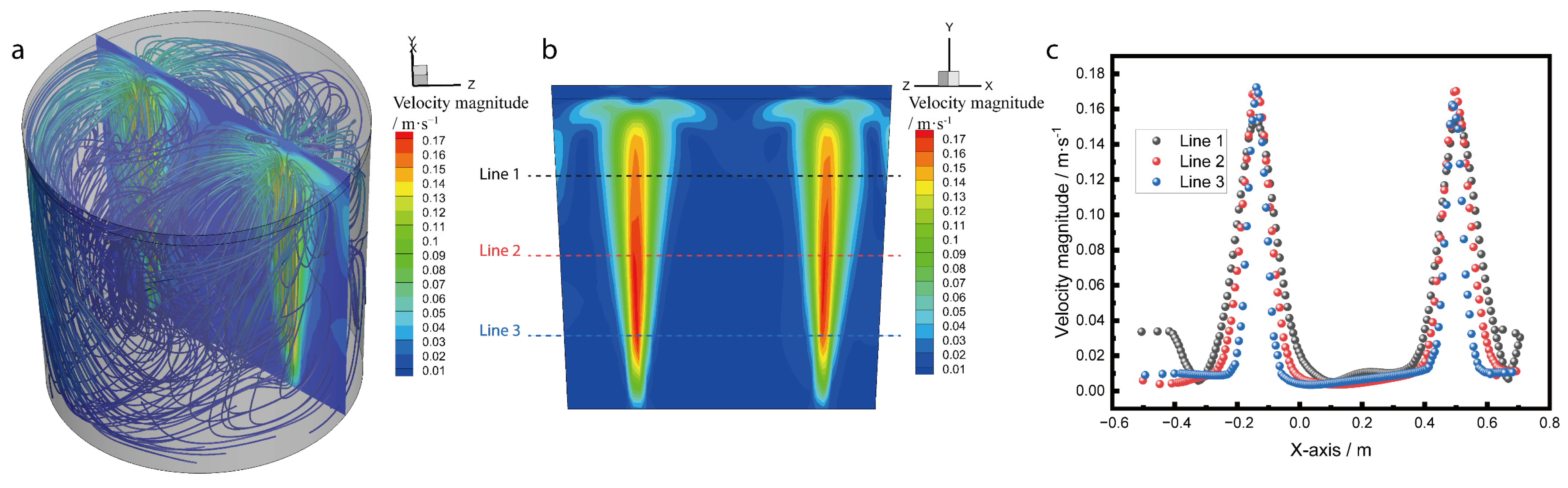
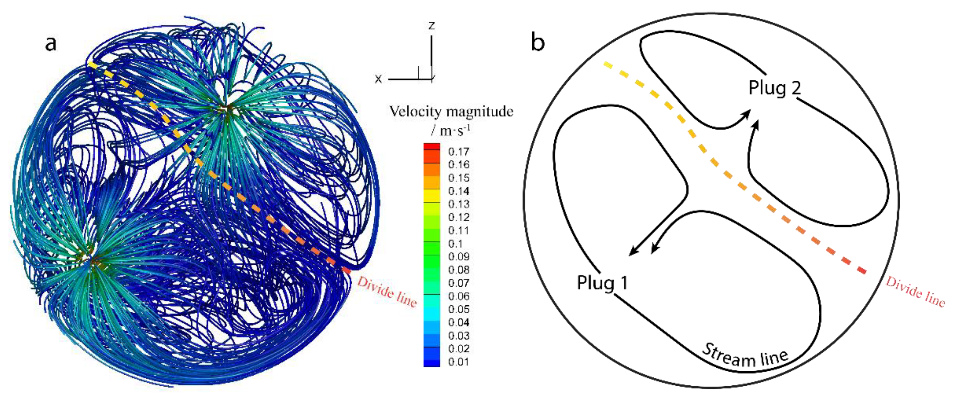
3.2.1. The Fluid Flows

Figure 8 shows the streamline, the slice position, and the quantitative data of the velocity magnitude in the prototype. Figure 8a shows the streamline and the sliced contour of the velocity. Figure 8a shows that the streamline flows from the ladle bottom where the plug is situated, the streamline is forward to the top of the ladle, and the streamline is reverse to the ladle bottom. Figure 8b shows that the velocity is higher in the bubble transport route, and the velocity magnitude is decreased near the surf of the ladle. The flow is divided into two streams when the stream flows to the surf of the ladle. Figure 8c shows the velocity magnitude in the three lines shown in Figure 8b. The results show that the stream velocity peak is broader in Line 1 compared to Lines 2 and 3. The maximum velocity in the stream is 0.172 m·s⁻¹.

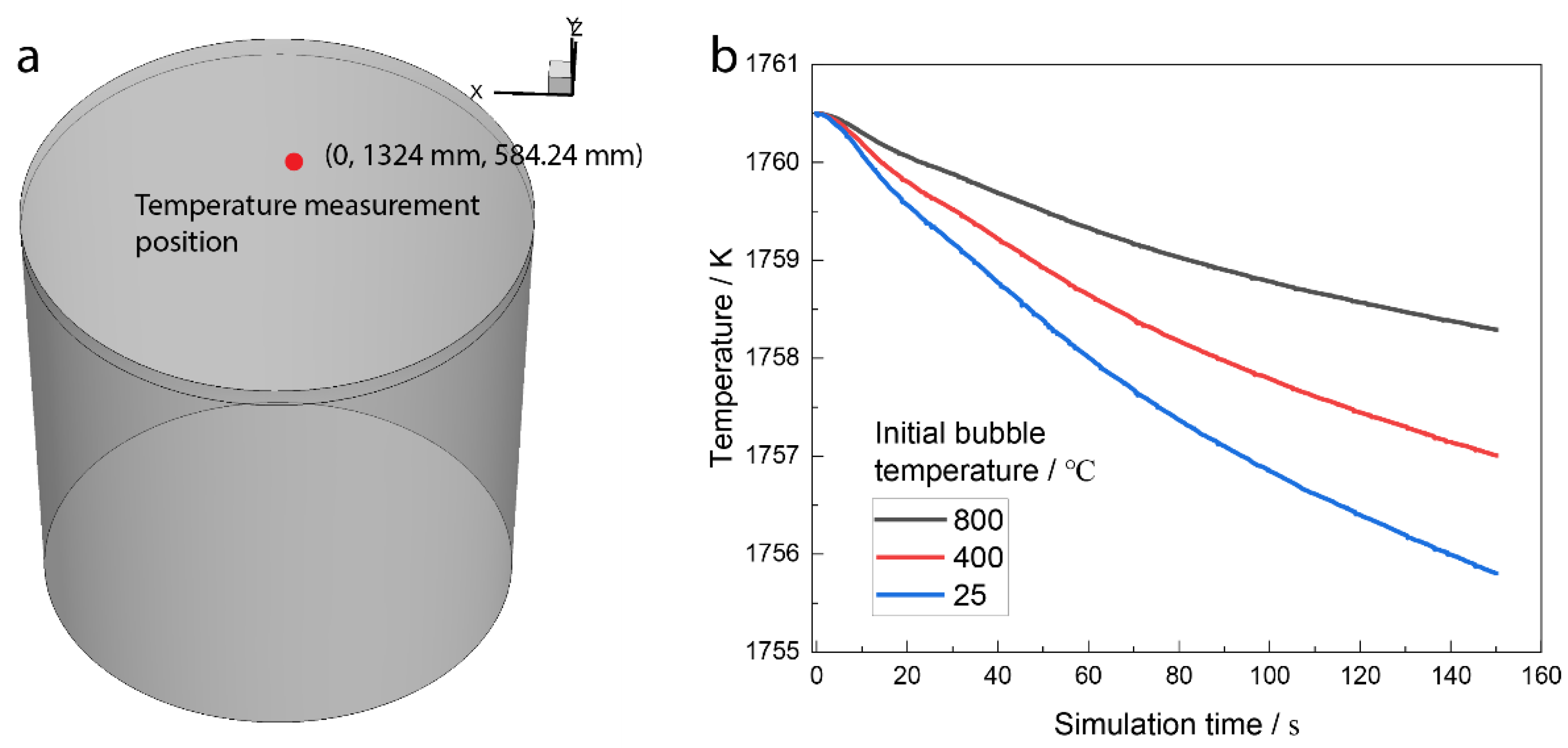
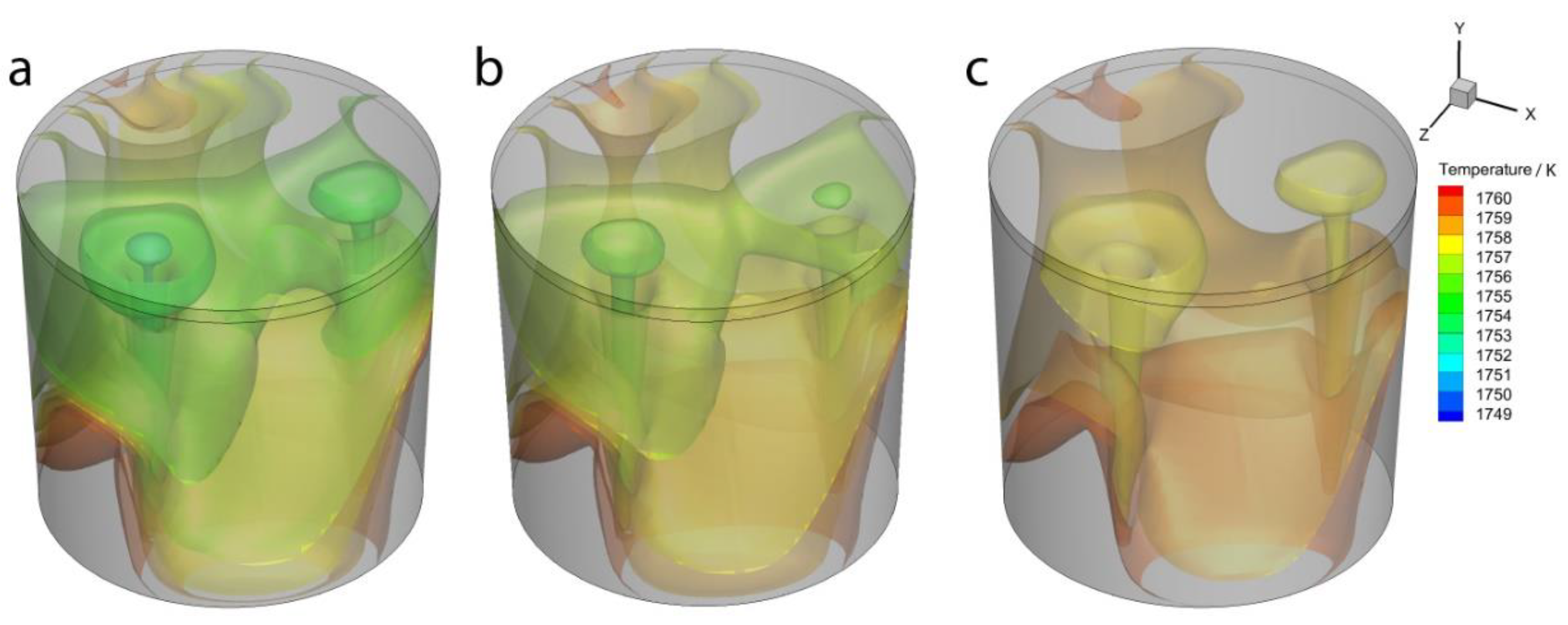
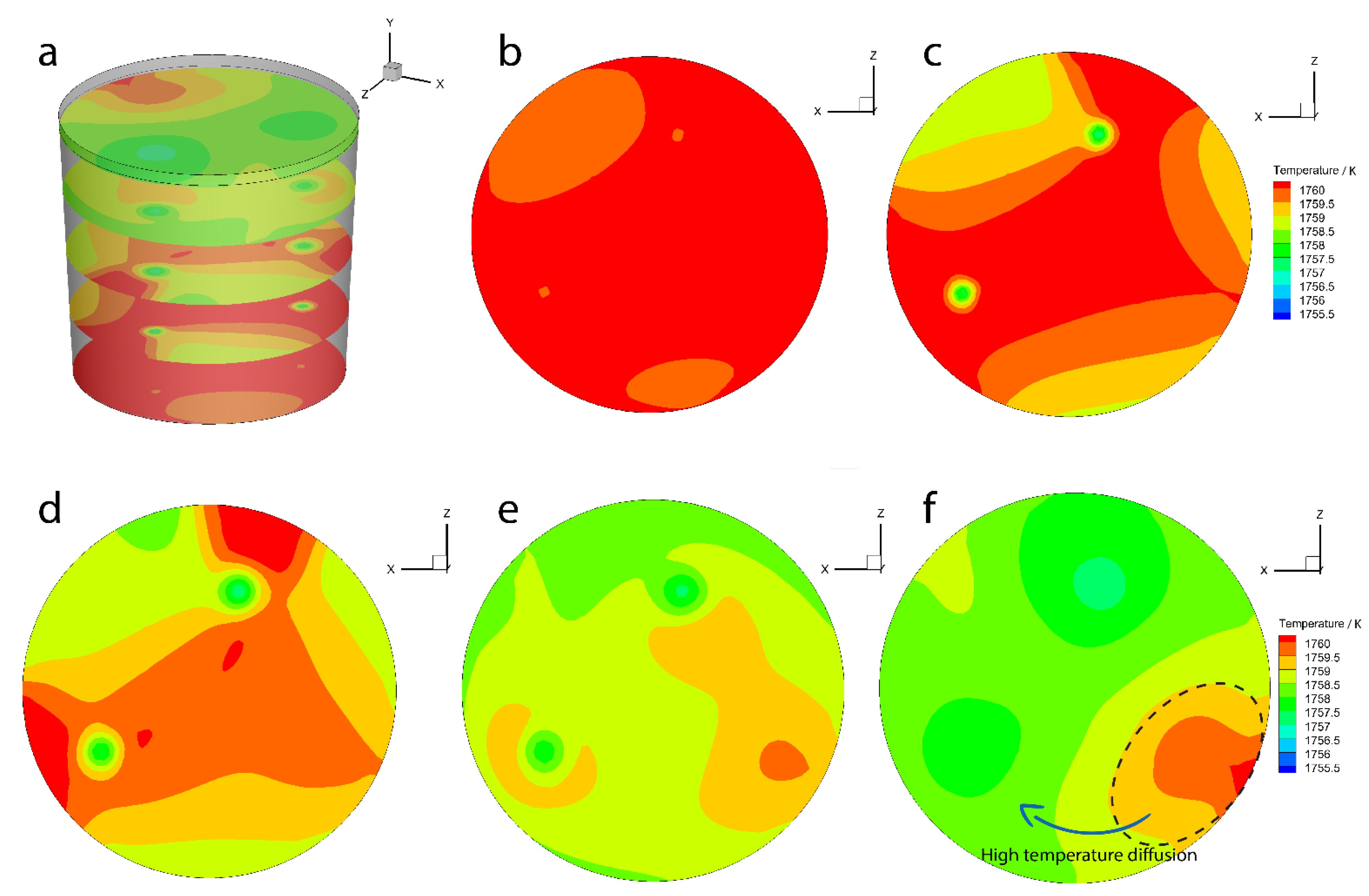
3.2.2. The Temperature Fields

Effect of Initial Bubble Temperature on the Temperature Filed

Figure 9 shows the temperature measurement position in industrial practice, and the numerical simulation of the temperature varies with the solution time at the temperature measurement position. In industrial practice, the temperature is 1759 K before the argon blow, and the temperature is 1740 K when the argon blow lasts for 22 min. The temperature drop rate is 0.0144 K/s. The bubble is injected from the ladle bottom, and then the bubble temperature is lower than that of the molten steel, which will decrease the molten steel temperature. Figure 9b shows the temperature variation with the solution time under different initial bubble temperatures. The temperature decrease rate is 0.0147 K/s, 0.023 K/s, and 0.0313 K/s when the initial bubble temperature is 800 °C, 400 °C, and 25 °C, respectively. The temperature decrease rate is increased when the initial bubble temperature decreases. The temperature decrease rate is similar to the industrial practice when the initial bubble injection temperature is 800 °C.

Figure 10 shows the iso-surface of the temperature under the different initial bubble temperatures when the argon blow simulation time lasts 150 s. The molten steel temperature is lower where the bubble is placed. The low-temperature area is diffused along the fluid flow direction.

Figure 11 shows the sliced contour of the temperature when the initial bubble temperature is 800 °C and the solution time is 150 s. The results show that the temperature in the ladle bottom is higher than those in the other slices. The temperature in the bubble plume area is lower than those in the different regions. The temperature distribution is asymmetric because the plugs distribution is asymmetric, which results in the flow being asymmetric. The high-temperature area is diffused to the low-temperature area.

Figure 12a shows the streamline in the top view of the ladle. The stream in the ladle is divided into two main circulations. Plug 1 is set at 0.67R_m and plug 2 is set at 0.6R_m. Figure 12b shows the schematic of the circulation, and the circulation is larger in plug 1. The circulation area is asymmetric, which results in the temperature field asymmetry. The temperature fields are diffused in the flow direction. The circulation area of plug 1 is larger than that of plug 2, then the molten steel temperature above plug 1 is higher, as shown in Figure 11f.

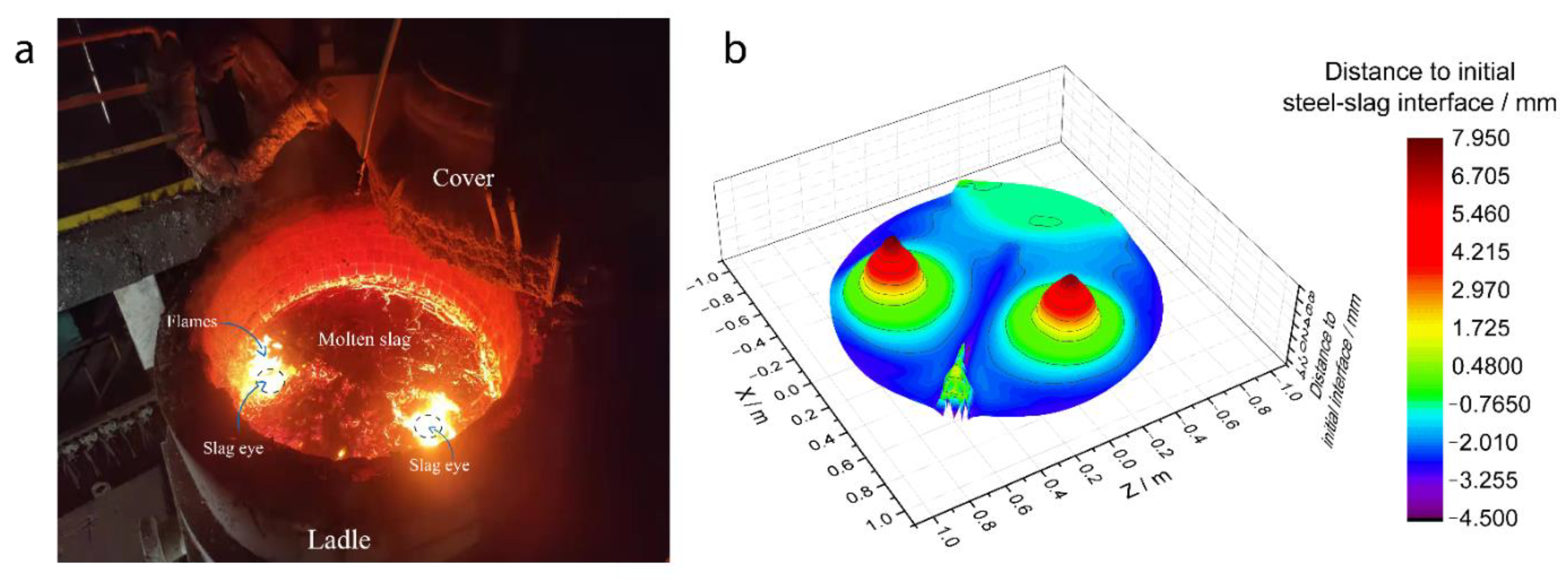
3.2.3. The Steel–Slag Interface Shape

Figure 13a shows the argon-stirred process in a steel plant. The ladle contains 25 t of molten steel. There are two plugs used in the argon-stirred process, and there are two places called ‘slag eyes’ plotted by blue dash circles. Figure 13b shows the simulation results of the steel–slag interface shape during the argon-stirred process, and there are two ‘peaks’ formed above the two plugs. The argon bubbles drive the fluid upward, then push the slag away, which results in the two ‘slag eyes’ formed. Figure 13b shows that the maximum height of the steel–slag interface is 7.95 mm, and the simulation results of the position of the ‘slag eyes’ are similar to industrial practice.

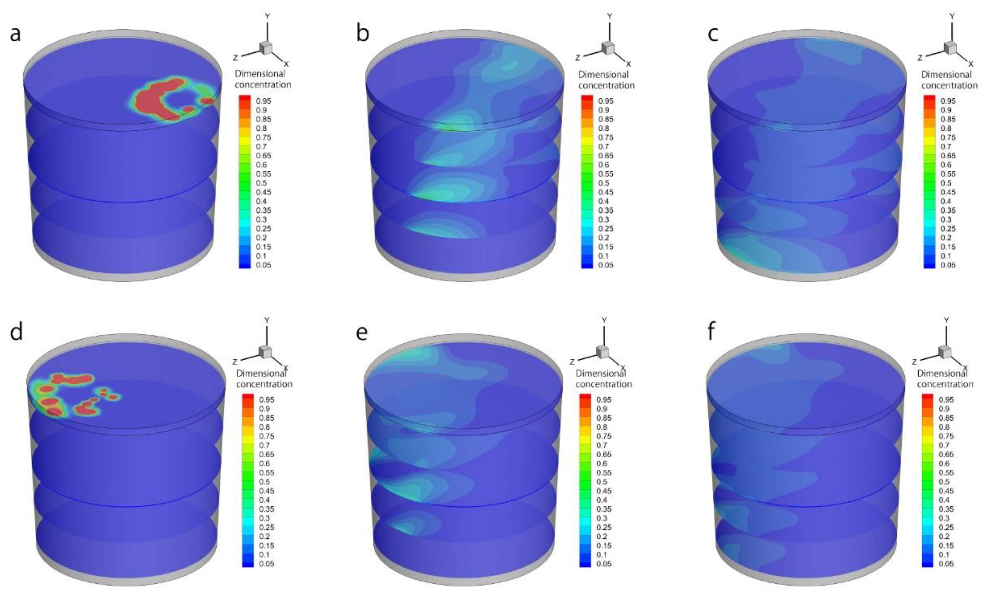
3.2.4. Alloy Melting and Alloy Species Diffusion

Figure 14 shows the sliced contour of the dimensional concentration. Figure 14a–c show the alloy added in the ‘slag eye’ above plug 1. The results show that the alloy melts and releases the species of the alloy, then the species is diffused along the fluid flow direction. Figure 14d–f show that the alloy added above the ‘slag eye’ is above plug 2.

Figure 15a,b show the alloy melting position when the alloy is added in the ‘slag eye’ above plug 1 and plug 2. Figure 15a,b show that the alloy melting position is in a circle shape, near the ‘slag eye’. Figure 15c shows the statistical results of the melting time, and the results show that the average melting time is 12.49 s and 12.71 s when the alloy added in the ‘slag eye’ is above plug 1 and plug 2, respectively. The melting time when the alloy is added in the ‘slag eye’ above plug 1 is less than that of plug 2. Figure 11f and Figure 12 show that the circulation area in plug 1 is higher than that of plug 2, the molten steel temperature in the ‘slag eye’ above plug 1 is higher than that of plug 2, and the melting time is decreased when the molten steel temperature increases. Figure 15d shows the average dimensional concentration varying with the solution time, and the average dimensional concentration is increased and reaches a maximum after the alloy is added after 20 s. The maximum of the average dimensional concentration is higher when the alloy is added on the ‘slag eye’ above plug 1, because the melting time is less, and the average dimensional concentration has fewer changes after the alloy is added after 100 s.

4. Conclusions

In this paper, a multi-physics numerical simulation model in an argon-stirred ladle was established, the random walk model was used in the bubble transport model, and the effect of C_L on the fluid flow simulation was studied for the first time. In the temperature simulation, a heat flux transfer model in molten steel and bubbles was introduced for the first time. The effect of initial bubble temperature on the molten steel temperature simulation was discussed. The alloy melting and alloy concentration diffusion were simulated. The multi-physics simulation model was beneficial in the ladle design and the modification of the parameters.

(1)

The random walk model needs to be applied to the bubble transport model. The velocity difference between the numerical simulation and the hydraulic model decreases when the C_L decreases from 0 to 0.3 and increases when the C_L increases from 0.3 to 0.45. The velocity difference between the numerical simulation and the hydraulic model is minimum when the C_L is 0.3.

(2)

There are two circulations of fluid flow in the prototype. The velocity is higher in the center of the plume. The velocity is smaller near the steel–slag interface. The maximum velocity is 0.172 m·s⁻¹.

(3)

The molten steel temperature will decrease when the argon bubbles are injected into the molten steel from the plugs. The temperature decrease rate will increase when the initial bubble temperature decreases. The temperature decrease rate in industrial practice is 0.0144 K/s. The numerical simulation results of the temperature decrease rate are 0.0147 K/s when the initial bubble temperature is 800 °C.

(4)

The steel–slag interface position is higher above the plugs. The maximum height of the steel–slag interface is 7.95 mm.

(5)

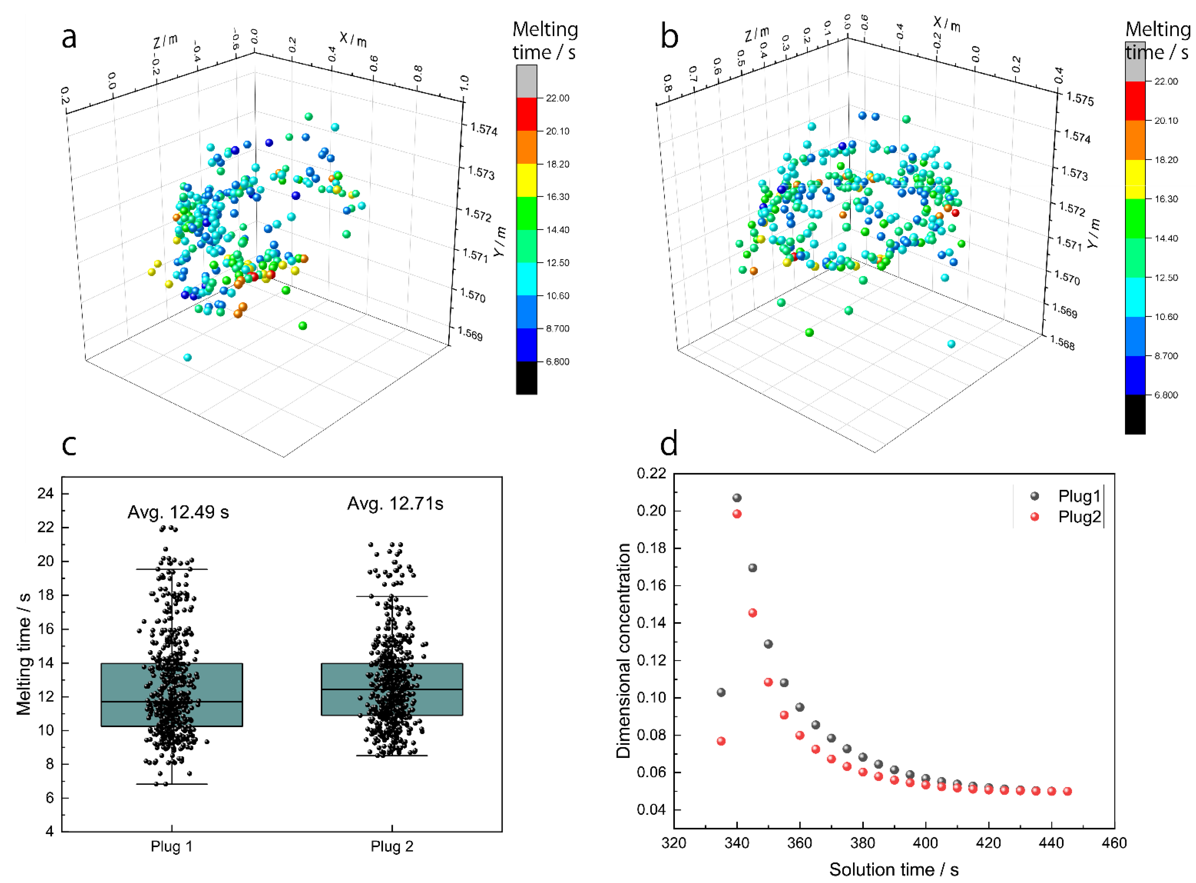
The average alloy melting time is 12.49 s or 12.71 s when the alloy is added on the two slag eyes separately. The alloy melting time has a little difference because the molten steel temperature has little difference in the two slag eyes. The average alloy concentration in the ladle is increased when the alloy is added to the molten steel in 20 s, and the average alloy concentration decreases during the alloy species diffusion. The alloy concentration has fewer changes when the alloy is added to the molten steel after 100 s.

References

1. Conejo, A.N.; Kitamura, S.; Maruoka, N.; Kim, S.J. Effects of Top Layer, Nozzle Arrangement, and Gas Flow Rate on Mixing Time in Agitated Ladles by Bottom Gas Injection. Metall. Mater. Trans. B 2013, 44, 914–923. [Google Scholar] [CrossRef]
2. Liu, Z.; Li, L.; Li, B. Modeling of Gas-Steel-Slag Three-Phase Flow in Ladle Metallurgy: Part I. Physical Modeling. ISIJ Int. 2017, 57, 1971–1979. [Google Scholar] [CrossRef] [Green Version]
3. Manuel Amaro-Villeda, A.; Aurelio Ramirez-Argaez, M.; Conejo, A.N. Effect of Slag Properties on Mixing Phenomena in Gas-stirred Ladles by Physical Modeling. ISIJ Int. 2014, 54, 1–8. [Google Scholar] [CrossRef] [Green Version]
4. Mazumdar, D.; Dhandapani, P.; Sarvanakumar, R. Modeling and Optimisation of Gas Stirred Ladle Systems. ISIJ Int. 2017, 57, 286–295. [Google Scholar] [CrossRef] [Green Version]
5. Szekely, J.; Wang, H.J.; Kiser, K.M. Flow Pattern Velocity and Turbulence Energy Measurements and Predictions in a Water Model of an Argon-Stirred Ladle. Metall. Trans. B 1976, 7, 287–295. [Google Scholar] [CrossRef]
6. Li, Y.; Zhu, H.; Wang, R.; Ren, Z.; He, Y. Bubble behavior and evolution characteristics in the RH riser tube-vacuum chamber. Int. J. Chem. React. Eng. 2022. [Google Scholar] [CrossRef]
7. Li, Y.; Zhu, H.; Wang, R.; Ren, Z.; Lin, L. Prediction of two phase flow behavior and mixing degree of liquid steel under reduced pressure. Vacuum 2021, 192, 110480. [Google Scholar] [CrossRef]
8. Pan, Q.; Johansen, S.T.; Olsen, J.E.; Reed, M.; Sætran, L.R. On the turbulence modelling of bubble plumes. Chem. Eng. Sci. 2021, 229, 116059. [Google Scholar] [CrossRef]
9. Mantripragada, V.T.; Sahu, S.; Sarkar, S. Morphology and flow behavior of buoyant bubble plumes. Chem. Eng. Sci. 2021, 229, 116098. [Google Scholar] [CrossRef]
10. Xu, Y.; Ersson, M.; Jonsson, P.G. A Numerical Study about the Influence of a Bubble Wake Flow on the Removal of Inclusions. ISIJ Int. 2016, 56, 1982–1988. [Google Scholar] [CrossRef] [Green Version]
11. Li, Y.-H.; Bao, Y.-P.; Wang, R.; Ma, L.-F.; Liu, J.-S. Modeling study on the flow patterns of gas-liquid flow for fast decarburization during the RH process. Int. J. Miner. Metall. Mater. 2018, 25, 153–163. [Google Scholar] [CrossRef]
12. Yuan, F.; Xu, A.-J.; Gu, M.-Q. Development of an improved CBR model for predicting steel temperature in ladle furnace refining. Int. J. Miner. Metall. Mater. 2021, 28, 1321–1331. [Google Scholar] [CrossRef]
13. Gu, C.; Liu, W.-Q.; Lian, J.-H.; Bao, Y.-P. In-depth analysis of the fatigue mechanism induced by inclusions for high-strength bearing steels. Int. J. Miner. Metall. Mater. 2021, 28, 826–834. [Google Scholar] [CrossRef]
14. Xiao, W.; Bao, Y.-Q.; Gu, C.; Wang, M.; Liu, Y.; Huang, Y.-S.; Sun, G.-T. Ultrahigh cycle fatigue fracture mechanism of high-quality bearing steel obtained through different deoxidation methods. Int. J. Miner. Metall. Mater. 2021, 28, 804–815. [Google Scholar] [CrossRef]
15. Li, Y.; He, Y.; Ren, Z.; Bao, Y.; Wang, R. Comparative Study of the Cleanliness of Interstitial-Free Steel with Low and High Phosphorus Contents. Steel Res. Int. 2021, 92, 2000581. [Google Scholar] [CrossRef]
16. Guo, X.; Godinez, J.; Walla, N.J.; Silaen, A.K.; Oltmann, H.; Thapliyal, V.; Bhansali, A.; Pretorius, E.; Zhou, C.Q. Computational Investigation of Inclusion Removal in the Steel-Refining Ladle Process. Processes 2021, 9, 1048. [Google Scholar] [CrossRef]
17. Krishnapisharody, K.; Irons, G.A. A Model for Slag Eyes in Steel Refining Ladles Covered with Thick Slag. Metall. Mater. Trans. B 2015, 46, 191–198. [Google Scholar] [CrossRef]
18. Patil, S.P.; Satish, D.; Peranandhanathan, M.; Mazumdar, D. Mixing Models for Slag Covered, Argon Stirred Ladles. ISIJ Int. 2010, 50, 1117–1124. [Google Scholar] [CrossRef] [Green Version]
19. Peranandhanthan, M.; Mazumdar, D. Modeling of Slag Eye Area in Argon Stirred Ladles. ISIJ Int. 2010, 50, 1622–1631. [Google Scholar] [CrossRef] [Green Version]
20. Conejo, A.N. Physical and Mathematical Modelling of Mass Transfer in Ladles due to Bottom Gas Stirring: A Review. Processes 2020, 8, 750. [Google Scholar] [CrossRef]
21. Hua, J.; Wang, C.-H. Numerical simulation of bubble-driven liquid flows. Chem. Eng. Sci. 2000, 55, 4159–4173. [Google Scholar] [CrossRef]
22. Chen, C.; Jonsson, L.T.I.; Tilliander, A.; Cheng, G.; Jönsson, P.G. A mathematical modeling study of the influence of small amounts of KCl solution tracers on mixing in water and residence time distribution of tracers in a continuous flow reactor-metallurgical tundish. Chem. Eng. Sci. 2015, 137, 914–937. [Google Scholar] [CrossRef]
23. Geng, D.-Q.; Lei, H.; He, J.-C. Optimization of mixing time in a ladle with dual plugs. Int. J. Miner. Metall. Mater. 2010, 17, 709–714. [Google Scholar] [CrossRef]
24. Li, L.; Liu, Z.; Li, B.; Matsuura, H.; Tsukihashi, F. Water Model and CFD-PBM Coupled Model of Gas-Liquid-Slag Three-Phase Flow in Ladle Metallurgy. ISIJ Int. 2015, 55, 1337–1346. [Google Scholar] [CrossRef] [Green Version]
25. Uriostegui-Hernandez, A.; Garnica-Gonzalez, P.; Angel Ramos-Banderas, J.; Alberto Hernandez-Bocanegra, C.; Solorio-Diaz, G. Multiphasic Study of Fluid-Dynamics and the Thermal Behavior of a Steel Ladle during Bottom Gas Injection Using the Eulerian Model. Metals 2021, 11, 1082. [Google Scholar] [CrossRef]
26. Mazumdar, D.; Guthrie, R.I.L. Modeling Energy Dissipation in Slag-Covered Steel Baths in Steelmaking Ladles. Metall. Mater. Trans. B 2010, 41, 976–989. [Google Scholar] [CrossRef]
27. Zhu, M.Y.; Inomoto, T.; Sawada, I.; Hsiao, T.C. Fluid-Flow and Mixing Phenomena in the Ladle Stirred by Argon through Multi-Tuyere. ISIJ Int. 1995, 35, 472–479. [Google Scholar] [CrossRef]
28. Liu, H.; Qi, Z.; Xu, M. Numerical Simulation of Fluid Flow and Interfacial Behavior in Three-phase Argon-Stirred Ladles with One Plug and Dual Plugs. Steel Res. Int. 2011, 82, 440–458. [Google Scholar] [CrossRef]
29. Llanos, C.A.; Garcia-Hernandez, S.; Ramos-Banderas, J.A.; Barret, J.D.J.; Solorio-Diaz, G. Multiphase Modeling of the Fluidynamics of Bottom Argon Bubbling during Ladle Operations. ISIJ Int. 2010, 50, 396–402. [Google Scholar] [CrossRef] [Green Version]
30. Tang, H.; Guo, X.; Wu, G.; Wang, Y. Effect of Gas Blown Modes on Mixing Phenomena in a Bottom Stirring Ladle with Dual Plugs. ISIJ Int. 2016, 56, 2161–2170. [Google Scholar]
31. Huang, A.; Gu, H.; Zhang, M.; Wang, N.; Wang, T.; Zou, Y. Mathematical Modeling on Erosion Characteristics of Refining Ladle Lining with Application of Purging Plug. Metall. Mater. Trans. B 2013, 44, 744–749. [Google Scholar] [CrossRef]
32. Li, L.; Li, B. Investigation of Bubble-Slag Layer Behaviors with Hybrid Eulerian-Lagrangian Modeling and Large Eddy Simulation. JOM 2016, 68, 2160–2169. [Google Scholar] [CrossRef]
33. Liu, W.; Tang, H.; Yang, S.; Wang, M.; Li, J.; Liu, Q.; Liu, J. Numerical Simulation of Slag Eye Formation and Slag Entrapment in a Bottom-Blown Argon-Stirred Ladle. Metall. Mater. Trans. B 2018, 49, 2681–2691. [Google Scholar] [CrossRef]
34. Xue, Z.L.; Wang, Y.F.; Wang, L.T.; Li, Z.B.; Zhang, J.W. Inclusion removal from molten steel by attachment small bubbles. Acta Metall. Sin. 2003, 39, 431–434. [Google Scholar]
35. Zhu, M.Y.; Zheng, S.G.; Huang, Z.Z.; Gu, W.P. Numerical simulation of nonmetallic inclusions behaviour in gas-stirred ladies. Steel Res. Int. 2005, 76, 718–722. [Google Scholar] [CrossRef]
36. Mantripragada, V.T.; Sarkar, S. Multi-Objective Optimization of Bottom Purged Steelmaking Ladles. Trans. Indian Inst. Met. 2022, 1–10. [Google Scholar] [CrossRef]
37. Cheng, R.; Zhang, L.; Yin, Y.; Ma, H.; Zhang, J. Influence of Argon Gas Flow Parameters in the Slot Plug on the Flow Behavior of Molten Steel in a Gas-Stirred Ladle. Trans. Indian Inst. Met. 2021, 74, 1827–1837. [Google Scholar] [CrossRef]
38. Bhattacharjee, A.; Mazumdar, D. Mathematical-Modeling of Fluid-Flow, Alloy Dissolution and Mixing in Industrial Argon Stirred Ladles. Trans. Indian Inst. Met. 1992, 45, 153–161. [Google Scholar]
39. Kwon, Y.-J.; Zhang, J.; Lee, H.-G. A CFD-based nucleation-growth-removal model for inclusion behavior in a gas-agitated ladle during molten steel deoxidation. ISIJ Int. 2008, 48, 891–900. [Google Scholar] [CrossRef] [Green Version]
40. Lachmund, H.; Xie, Y.K.; Buhles, T.; Pluschkell, W. Slag emulsification during liquid steel desulphurisation by gas injection into the ladle. Steel Res. Int. 2003, 74, 77–85. [Google Scholar] [CrossRef]
41. Singh, U.; Anapagaddi, R.; Mangal, S.; Padmanabhan, K.A.; Singh, A.K. Multiphase Modeling of Bottom-Stirred Ladle for Prediction of Slag-Steel Interface and Estimation of Desulfurization Behavior. Metall. Mater. Trans. B 2016, 47, 1804–1816. [Google Scholar] [CrossRef]
42. Wondrak, T.; Timmel, K.; Bruch, C.; Gardin, P.; Hackl, G.; Lachmund, H.; Lungen, H.B.; Odenthal, H.-J.; Eckert, S. Large-Scale Test Facility for Modeling Bubble Behavior and Liquid Metal Two-Phase Flows in a Steel Ladle. Metall. Mater. Trans. B 2022, 53, 1703–1720. [Google Scholar] [CrossRef]
43. Uriostegui-Hernandez, A.; Garnica-Gonzalez, P.; Hernandez-Bocanegra, C.-A.; Ramos-Banderas, J.-A.; Montes-Rodriguez, J.-J.; Ortiz-Castillo, J.-R. Study of fluid dynamics and sulfar mass transfer between steel and slag in a ladle furnace considering drag and non-drag forces. Dyna 2022, 97, 176–183. [Google Scholar] [CrossRef]
44. Wang, Q.; Liu, C.; Pan, L.; He, Z.; Li, G. Numerical Understanding on Refractory Flow-Induced Erosion and Reaction-Induced Corrosion Patterns in Ladle Refining Process. Metall. Mater. Trans. B 2022, 53, 1617–1630. [Google Scholar] [CrossRef]
45. Joubert, N.; Gardin, P.; Popinet, S.; Zaleski, S. Experimental and numerical modelling of mass transfer in a refining ladle. Metall. Res. Technol. 2022, 119, 109. [Google Scholar] [CrossRef]
46. Riabov, D.; Gain, M.M.; Kargul, T.; Volkova, O. Influence of Gas Density and Plug Diameter on Plume Characteristics by Ladle Stirring. Crystals 2021, 11, 475. [Google Scholar] [CrossRef]
47. Li, Q.; Pistorius, P.C. Interface-Resolved Simulation of Bubbles-Metal-Slag Multiphase System in a Gas-Stirred Ladle. Metall. Mater. Trans. B 2021, 52, 1532–1549. [Google Scholar] [CrossRef]
Figure 1. The schematic of the velocity measurement setup.
Processes 10 01563 g001
Figure 2. Schematic of the simulation model in the argon-stirred ladle.
Processes 10 01563 g002
Figure 3. Hexahedral mesh of the fluid zone, boundary name, boundary condition, and the schematic of the argon injection position: (a) prototype; (b) hydraulic model.
Processes 10 01563 g003
Figure 4. (a) The slice position of the simulation results of the water model, (b) the velocity magnitude contour in the slice when the random walk model was deactivated, (c) the velocity magnitude contour in the slice when the random walk model was activated and the CL was 0.15, and (d) the time-averaged results of the PIV measurements in the water model.
Processes 10 01563 g004
Figure 5. The quantitative velocity magnitude data of numerical simulation of water model and PIV measurements results, when the random walk model was deactivated (a) near the water surface, (b) under the water surface by 100 mm, and (c) under the water surface by 200 mm; when the random walk model was activated and the CL was 0.15 (d) near the water surface, (e) under the water surface by 100 mm, and (f) under the water surface by 200 mm.
Processes 10 01563 g005
Figure 6. The quantitative velocity magnitude data of numerical simulation of water model and PIV measurements results, when the random walk model was activated and CL was 0.3 (a) near the water surface, (b) under the water surface by 100 mm, and (c) under the water surface by 200 mm; when the random walk model was activated and the CL was 0.45 (d) near the water surface, (e) under the water surface by 100 mm, and (f) under the water surface by 200 mm.
Processes 10 01563 g006
Figure 7. The variance in the velocity difference between PIV measurements and numerical simulation at −100 mm to 100 mm in Figure 5 and Figure 6.
Processes 10 01563 g007
Figure 8. The prototype numerical simulation results: (a) streamline results and slice contour position, (b) velocity contour at the slice position, and (c) velocity magnitude results at three lines.
Processes 10 01563 g008
Figure 9. (a) Temperature measurements position in the industrial practice; (b) temperature varies with solution time at the temperature measurements position.
Processes 10 01563 g009
Figure 10. The temperature iso-surface under different initial bubble temperatures: (a) 25 °C, (b) 400 °C, and (c) 800 °C.
Processes 10 01563 g010
Figure 11. The temperature slice contour when the initial bubble temperature is 800 °C: (a) slice position, (b) slice position near the bottom, (c) slice position at Y = 0.3935, (d) slice position at Y = 0.787, (e) slice position at Y = 1.18, and (f) slice position at near the surface.
Processes 10 01563 g011
Figure 12. (a) The streamline in the top view; (b) the schematic of the streamline in the different plugs.
Processes 10 01563 g012
Figure 13. (a) The molten steel and slag surface during the argon-stirred process, and (b) the numerical simulation results of the steel–slag interface position.
Processes 10 01563 g013
Figure 14. The contour of the slice of the dimensional concentration of the alloy species in the ladle when the alloy is added on the ‘slag eye’ above plug 1, after (a) 10 s, (b) 65 s, and (c) 120 s; when the alloy is added on the ‘slag eye’ above plug 2, after (d) 10 s, (e) 65 s, and (f) 120 s.
Processes 10 01563 g014
Figure 15. The alloy melting position when the alloy is added on the ‘slag eye’ above (a) plug 1 and (b) plug 2; (c) the alloy melting time and (d) the average dimensional concentration under different alloy add-in positions.
Processes 10 01563 g015