Abstract
To obtain quality variables that cannot be measured in real time during the production process but reflect information on the quality of the final product, the batch production process has the characteristics of a strong time-varying nature, non-Gaussian data distribution and high nonlinearity. A locally weighted partial least squares regression quality prediction model (KICA-JITL-LWPLS), based on wavelet kernel function independent meta-analysis with immediate learning, is proposed. The model first measures the similarity between the normalized input data and the historical data and assigns the input data to the group of historical data with high similarity to it, based on the posterior probability of the Bayesian classifier; subsequently, wavelet kernel functions are selected and kernel learning methods are introduced into the independent meta-analysis algorithm. An independent meta-analysis, based on the wavelet kernel function, is performed on the classified input data to obtain probabilistically significant independent sets of variables. Finally, a real-time learning-based LWPLS regression analysis is performed on this variable set to construct a local prediction model for the current sample by calculating the similarity between the local input data. The local predictions from the PLS output are fused with the posterior probability output from the Bayesian classifier to produce the final prediction. The method was used to predict the product concentration and bacteriophage concentration during penicillin fermentation through a simulation platform. The prediction results were basically consistent with the real values, proving that the proposed KICA-JITL-LWPLS quality prediction model, based on wavelet kernel functions, has reliable prediction results.
1. Introduction
Chemical, biological, and pharmaceutical processes are typically intermittent production processes. Producing products of consistent quality not only generates high profits for companies but also increases the visibility and recognition of their brands. Research in product quality is pivotal to the development of our manufacturing industry. In the intermittent production process, there are many important parameters and process variables that largely affect the final product quality and must be obtained and controlled. Due to current economic and technical constraints, these variables are difficult to measure online by sensors. The existing method of obtaining quality variables is to wait until the end of production, take samples by hand, and send them to the laboratory for analysis and testing [1,2]. This method has a serious lag, so it is necessary to predict the quality of the reaction process. To address this problem, experts have proposed soft measurement techniques that are computationally simple, do not require knowledge of the reaction mechanism or a priori knowledge of the production process, and are suitable for handling high-dimensional data [3,4,5].
Currently, data-driven soft measurement techniques, such as PCA (principal component analysis), ICA (independent component analysis), KICA (kernel independent component analysis), etc., have been widely used in the data processing of intermittent production process quality prediction [6,7]. Among them, the PCA algorithm takes advantage of the uncorrelated variables and extracts the linear uncorrelated variables from a few high-dimensional original variables to construct a linear regression model with the dependent variable instead of the original variables. However, the principal meta-analysis assumes a Gaussian linear distribution of the sample data in the selection of data features, which is inconsistent with actual production, resulting in such methods failing to provide accurate predictive performance [8,9,10]. Therefore, ICA algorithms were proposed [11], and, initially, ICA algorithms were used to separate mixed data, assuming that the mixed data obeyed a non-Gaussian distribution and that ICA algorithms could greatly guarantee the independence of the extracted components in a probabilistic sense while reducing the dimensionality of the original data, and the performance of this independence was much greater than the irrelevance required by PCA algorithms to extract principal elements. This is why the ICA algorithm is widely used in the field of data processing for non-Gaussian industrial processes [12,13]. Although the ICA algorithm achieves the purpose of processing non-Gaussian data, the ICA algorithm has limitations in the selection of the contrast function. Most of the classical studies of the ICA algorithms are based on variable contrast functions that are based on the expectation for a single and fixed non-linear function whose key property is that the separation of independent components is achieved when, and only when, the contrast function is equal to zero [14,15]. This approach does not provide high accuracy in solving complex non-linear forms of data-separation problems. To solve this problem, the kernel learning method was introduced into the ICA algorithm to extend the comparison function to the RKHS (reproducing kernel Hilbert space) for solving, which enhances the ability of the ICA algorithm to solve nonlinear problems and can obtain better separation results [16,17,18]. The introduction of kernel learning methods inevitably involves the selection of kernel function types, and most of the existing KICA algorithms are based on conventional kernel functions for exposition; however, conventional kernel functions cannot produce a complete substrate in high-dimensional space after passing the mapping, and they themselves tend to be mutually redundant when performing data analysis, limiting the improvement of the separation performance of KICA algorithms. Therefore, a new kernel function is needed to obtain a better interpretation of the nonlinearity [19,20]. The wavelet kernel function, by virtue of the multi-scale nature of the wavelet transform and by providing an approximate orthogonal basis, combined with the ICA algorithm to analyze the data step-by-step, can improve the ability of the non-linear mapping and hence the data separation performance [21,22]. Although the above methods can handle non-Gaussian and complex non-linear data and improve the data-processing accuracy, they mainly emphasize the ability to interpret the independent variables themselves and ignore the ability to interpret the dependent variables [23,24]. It is often applied to fault detection and the data processing of industrial processes and is unable to perform regression analysis and build quality prediction models for the dependent variable.
ANN (artificial neural network) is a computational model or data model, which mainly uses the biological neural network structure and function and uses this topology to study the relationship between nodes or objects. Although the neural network has a strong fault tolerance, its prediction accuracy is higher than that of the multiple regression model. In neural networks, such as RBF (radial basis function) neural network, it contains one input layer, one hidden layer, and one output layer. The hidden layer is composed of a set of radial basis functions, which are generally Gaussian functions. For complex problems and high-dimensional input variables and research data with many similar attributes, using neural network prediction will greatly increase the size of the network, increase the computing time, and reduce the convergence and generalization ability of the network. Therefore, the neural network is more suitable for quality prediction with a long period, such as air quality prediction, etc. It is not suitable for industrial production processes where real-time performance is emphasized and historical data are less so. The algorithm based on the multiple regression model simplifies many change factors that affect the final quality in the process of realizing quality prediction and makes many assumptions in the training process of realizing the prediction, which is more efficient and has better real-time performance. Kim S, Kano M and, Nakagawa H et al. proposed a JITL-LWPLS (JITL locally weighted partial least squares) modeling method based on PLS (partial least squares regression), which incorporates the idea of JITL (just-in-time learning) [25]. In particular, the PLS algorithm allows the extracted score vector to explain the characteristics of the dependent variable to the greatest extent possible while maintaining the ability to explain the dependent variable [26]. Useful information can be extracted from large amounts of data to find and model process quality characteristics. The JITL based on the local weighting algorithm can reduce the impact of samples with low similarity on the model accuracy by considering the weights of input test points and historical data in the database during the modelling process through similarity measurements [27]. Reliable modelling results are achieved by building a local linear model of each datum measured to approximate the non-linear process [28,29,30]. However, such partial least squares-based algorithms are limited in their feature selection, assuming that the sample data are Gaussian distributed and the process data are linear, resulting in the inability of such methods to provide accurate prediction performance.
Aiming at the above problems, this paper proposes a KICA-JITL-LWPLS quality prediction model based on wavelet kernel function. The predictive model provides a new wavelet kernel function independent element analysis method and a dual similarity measure, and the prediction model balances the problem that the KICA algorithm can handle non-Gaussian, non-linear data but is unable to perform regression analysis on the dependent variable, resulting in inaccurate quality prediction. The JITL-based partially weighted partial least squares algorithm for quality prediction is able to perform regression analysis on both the independent and dependent variables but is unable to handle non-Gaussian, non-linear data, resulting in inaccurate modelling. When new data are input, the model first measures the similarity between the normalized input data and the historical data and assigns the input data to the historical data group with high similarity to it, based on the posterior probability of the Bayesian classifier; subsequently, wavelet kernel functions are selected and kernel learning methods are introduced into the independent meta-analysis algorithm. Independent meta-analysis based on the wavelet kernel function is performed on the classified input data to obtain probabilistically significant independent sets of variables; finally, an immediate learning-based LWPLS (locally weighted partial least squares) regression analysis was performed for this variable group. The similarity between local input data according to the similarity measure of Euclidean distance is calculated. Based on the similarity, the samples are instructed to assign priority to construct a local prediction model for the current sample. The local predictive value of the partial least square regression output is fused with the posterior probability output of the Bayesian classifier to produce the final prediction. The Pensim penicillin fermentation simulation platform verified that the proposed model can achieve accurate prediction of the bacteriophage concentration and penicillin concentration with a reduced RMSE (root mean square error) value of 0.1147 and 0.2228, respectively, compared to the traditional model.
2. Theoretical Basis
2.1. Algorithm Principle of ICA and KICA
Common quality prediction methods, such as partial least squares or principal element analysis, treat process variables with the assumption that they follow a Gaussian distribution. However, most process data in real industrial production are non-Gaussian distributed [31]. This makes traditional PLS or PCA algorithms ineffective in quality prediction. In contrast to PLS or PCA algorithms, which can only extract information about the covariance of the data and require high selection of input variables, too much extraction of principal components will increase the interaction between variables, while too little extraction of principal components will lead to the loss of important information and reduce the model accuracy [32]. The ICA algorithm yields probabilistically independent sets of variables that are more independent of each other than the uncorrelated nature of algorithms, such as PCA or PLS. A new partial least squares regression model was built by reselecting the sample on the basis of the group of independent variables, allowing for a great diversity of variable selection and model accuracy [33]. Assuming a process data matrix of , the basic independent meta-decomposition model is:
In the formula: is random observation signals, and is the corresponding source signal. is the mixing matrix; is the residual matrix. Suppose is a full rank matrix, then makes . At this point, the goal is to find the mixing matrix, , recover the source signal, , from the observed signal , and make the estimated independent of each other. The main idea is to establish the objective function, , with as the variable; the extreme value of is found by the optimization method, and the final mixing matrix is obtained when takes the extreme value. At present, the methods of estimating the mixture matrix criterion mainly include the methods of maximizing non-Gaussian, minimizing mutual information, and estimating the maximum likelihood function. However, using mutual information as a comparison function does not require any assumptions about the data and is more conducive to calculation. Therefore, this paper chooses to minimize mutual information as a unified measure of independence. If, and only if, the mutual information is equal to zero, are the sums of the components independent of each other.
Although the ICA algorithm achieves the purpose of processing non-Gaussian data, the ICA algorithm has limitations in the selection of contrast functions. Most of the research on the classic ICA algorithm is based on variable contrast functions, which are based on a single- and fixed-contrast function. The key properties of the desired form of the nonlinear function are the separation of independent components if, and only if, the contrast function is equal to zero. This method does not have high accuracy in solving complex nonlinear data separation problems. In order to solve this problem, the kernel learning method was introduced into the ICA algorithm, and the KICA algorithm was proposed. The contrast function was extended to the RKHS space for solving, which enhanced the ICA method’s ability to solve nonlinear problems and achieved better separation effects [34]. If is the Mercer kernel function on the data space, , its Gram matrix is positive semi-definite for any element in . Then, all kernel functions can be represented by the mapping relationship, , from data space , to data space .
RKHS space is a feature space with the properties shown in the above formula. The typical correlation coefficient in the data space is extended to the feature space by using the mapping of the kernel function for analysis, and a new statistical independence in the kernel space is obtained. The measure of the property is the kernel canonical correlation coefficient . If and represent observations of and , respectively, and , respectively, represent their images in the feature space. If the data in the feature space have been centralized, assumption represents the largest kernel canonical correlation coefficient in the finite sample of experience. For the fixed mapping relationship and of the feature space, the empirical covariance coefficient in the feature space can be written in the following form:
If and , respectively, represent the linear space obtained by extending the points of the data space through the mapping of , we can obtain , , where and are orthogonal to and , respectively. Combined with the definition of the canonical correlation coefficient, it is known that the covariance in the feature space needs to be calculated to analyze the canonical correlation in the feature space. If the expression form of the kernel Gram matrix is used, the covariance in the feature space can be expressed as the following formula.
The maximum kernel canonical correlation coefficient mapped to the feature space can then be obtained:
Among them, and are the kernel Gram matrices corresponding to and . , is the coefficient matrix corresponding to the covariance matrix.
2.2. LWPLS
Most nonlinear systems are only partially modeled according to the sample data information input at a certain time. However, the complexity of this fitting method increases exponentially as the dimension of the input vector increases, resulting in a slow learning rate. The nonlinear system theory holds that, if the output surface of the system is smooth, then any nonlinear system can be approximated by some local linear models [35]. Based on the receptive field local weighted regression (RFWR) algorithm, multiple local models fit nonlinear functions in different regions to fit the entire space, and the LWPLS algorithm is proposed by combining local models and soft sensing techniques [36]. The LWPLS algorithm performs partial least squares regression fitting inside the local model and uses an iterative form to process the newly input sample data, so that the newly input sample data will only affect a few parameters in the local model. If the weights obtained by the sample data in all local models do not exceed the set threshold, a new local model is added. If the weights obtained by the sample data in the two local models exceed the set threshold, then remove a local model based on weights. LWPLS can automatically increase or decrease the number of local models according to the demand, which can effectively avoid the mutual influence of old and new data. If the input/output variable matrix is , , the output predicted value is . The LWPLS model is:
where is the number of input variables, is the number of output variables, and is the number of input samples. The th input/output variable matrix is and , is the load matrix, principal component matrix, is the regression matrix, and , is the residual matrix.
3. A Kica-Jitl-Lwpls Quality Prediction Model Based on Wavelet Kernel Functions
3.1. JITL-Based LWPLS
JITL is a local modelling strategy that can effectively handle industrial processes with frequent state changes. In JITL-based algorithms, data pre-processing and model parameter estimation are performed in the offline phase, and modelling is moved to the online phase [37]. This modelling approach improves the real-time accuracy of the model. The basic JITL algorithm process can be divided into the following three steps:
- Store the newly obtained input/output data in the database;
- Use the nearest neighbor method to calculate the similarity between the new input data and the data in the database to estimate the value of the output variable, and use the selected relevant data to build a local model;
- Calculate the model output based on the current data and replace the previous data with the new data after the calculation.
The operation is repeated with new data. Accordingly, the following properties of the instantaneous learning strategy are also present:
- Similarity selection and modelling of the data are only started after a new sample is acquired;
- Similar samples are selected from the historical database to train the data required for modelling;
- The current model is valid only for the current sample point. For the data, , to be tested at a given moment, the similarity of to the data in the historical database is calculated by the JITL algorithm based on similarity detection.
The similarity indicates which historical samples are assigned priority to construct the local model for the current query sample [38]. Typically, the lower the similarity between the history sample and the query sample, the greater the distance, and vice versa. If the history sample has a greater similarity weight than the other samples, it will be selected as the local model sample in preference. The Euclidean distance is generally used as the basis for selection. Let the th input sample deposited in the database be , and for the newly detected data point, , its similarity with each sample point in the database is calculated as follows:
is the standard deviation of , is a positional parameter, generally being 0.1–0.5. Calculated from the above formula, is expressed in the form of a similarity matrix as , where , .
In the traditional JITL method modeling, all the collected historical input/output data are mixed together. When there are new data points, a local model based on the Euclidean distance similarity measurement method is established directly according to the historical input/output data. The output of the local model is the predicted output. This method is not very accurate. In this paper, the Bayesian classifier is combined for double similarity measurement to improve the accuracy of similarity detection. Bayesian classifiers belong to supervised learning, which builds corresponding probability models by learning training samples of known categories [39]. First, the data collected in different stages is collated into the database corresponding to the stage . Then, through the learning of the data in each database, a Bayesian classifier is induced. When it is necessary to predict the output estimated value of the newly arrived data point, , it is first divided into the sub-database to which it belongs according to the posterior probability value of the Bayesian classifier, and then, the kth LWPLS based on the Euclidean similarity measure is established according to the kth databases model. When new data points, , and class variables, , are measured online, the posterior probability that the data point belongs to each database is calculated for effective classification. The posterior probability calculation formula is as follows:
where , is the priori probability, is the attribute variable, and and are the mean and standard deviation of when .
3.2. KICA Algorithm Based on Wavelet Kernel Function
Existing kernel functions, such as the Gaussian kernel function and polynomial kernel function, cannot generate a complete basis in high-dimensional space after mapping, so the classifier cannot approximate any classification interface or classification curve in the space. For this, a new kernel function is needed to generate a complete basis in high-dimensional space. In this paper, by virtue of the multi-scale nature of the wavelet kernel function and the characteristics of providing an approximate orthonormal basis, with the help of the minimization of mutual information theory, by finding an approximate approximation of the kernel canonical correlation coefficient, the large-scale data problem is reduced to a finite number of empirical samples and analyzed to improve the ability of nonlinear mapping [40]. With the help of the invariance of the kernel translation, the measure of the non-Gaussian vector in the original vector can be derived from the mutual information of the Gaussian vector. Considering two Gaussian-free vectors, , , whose dimensions are , , the mutual information can be expressed as:
If the covariance matrix of , is , then the mutual information can be further expressed as:
Extending the mutual information to m Gaussian-free vectors, the mutual information is expressed as:
where is the generalized variance.
By Formula (6), and extending the problem to m vectors, the problem of solving the maximum kernel canonical correlation coefficient in the above formula is transformed to solve the kernel generalized eigenvalue problem as shown below:
Let denote the m-dimensional diagonalized matrix to the right of the equal sign; is the smallest kernel generalized eigenvalue in which if, and only if, is equal to 1, is equal to 0. At this time, the vectors are independent of each other, and the separation of independent components can be accomplished by defining a contrast function and minimizing the contrast function.
A support vector kernel function to obtain a permissible multidimensional tensor product:
, is the scale factor, , , , , , . The input of each dimension is formed into a kernel function in the form of a product, which reflects the local analysis of each dimension of the input and the multi-resolution relationship of each dimension of the wavelet kernel function. The steps of the KICA algorithm based on the wavelet kernel function are as follows:
Input as observational data ;
Step 1. Centralization and whitening ;
Step 2. Calculate a set of original independent data by , and calculate the corresponding wavelet kernel Gram matrix ;
Step 3. Compute kernel generalized variance , where is ;
Step 4. Minimize the contrast function . The signal independence is maximized by obtaining the corresponding to the global optimal solution.
3.3. The Steps of Kica-Jitl-Lwpls Algorithm Based on Wavelet Kernel Function
Let , represent the input and output variables of the quality predictive modeling sample set, respectively. Both are stored in the historical database. is the total number of samples, and is the number of input variables. The steps of the wavelet kernel function KICA-JITL-LWPLS algorithm are as follows:
Step 1. Divide the total sample into two parts; one part is the training sample set, and the other part is the validation set. Use training set samples for model prediction validation of set samples;
Step 2. In the training sample set, the KICA algorithm, based on the wavelet kernel function in the first section, is used to separate the source signal of the same dimension from the observed sample signal, extract the independent variables, re-sample the extracted variable group, and use the new sample to build a JITL-based LWPLS sub-model;
Step 3. Determine the latent variable ; the value of is the value corresponding to the minimum sum of the squares of the prediction error, and is the bandwidth parameter in the calculation of the training sample weight, which can be determined by the cross-validation method;
Step 4. Calculate the similarity matrix by Formulas (7) and (8);
Step 5. Calculate the input, output, incoming data point matrices , , ;
where is a column vector of all ones, , ;
Step 6. Let be the number of iteration steps, and set the initial value of to 1, , , , . Let perform the following iterative calculation from 1 to to obtain a local linear model;
The th score vector of :
The th score vector of query sample :
Calculate the th load vector of and the regression coefficient of :
Step 7. update output value;
Step 8. If , output ; otherwise, order ;
Step 9. Through the above steps, the output predicted value of the new data point is obtained, . Fusion with the posterior probability, , obtained by the Bayesian classifier outputs the final predicted value :
The RMSE is used as a performance indicator to evaluate the predictive ability of the modeling method in this paper. The calculation formula is as follows:
where is the true value, is the predicted value, and is the number of test data points. A flow chart of the KICA-JITL-LWPLS algorithm, based on the wavelet kernel function, is shown in Figure 1.
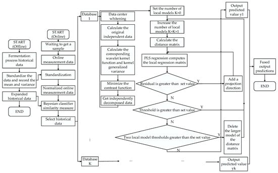
Figure 1.
Flowchart of the KICA-JITL-LWPLS algorithm based on wavelet kernel functions.
4. Simulation Example
Penicillin is an antibiotic used by humans on a large scale for clinical purposes; its production data process is non-Gaussian and its production process is a typical non-linear, dynamic, multi-stage intermittent production process [41]. The Pensim simulation platform used in this paper was developed by the process modelling, monitoring, and control group at the IIT (Illinois Institute of Technology), with Professor Cinar as the subject leader [42]. The simulation platform is an exe file that runs independently in the Windows environment; the kernel of the software adopts the improved Birol model based on the Bajpai mechanism model. Users can perform operations, such as data input, result display, and data export, on the interface. This simulation platform can easily implement a series of monitoring, fault-diagnosis, and quality-prediction simulations of the penicillin fermentation process, and relevant studies have demonstrated the practicality and effectiveness of this simulation platform [43].
In this experiment, batch data are generated by pensim software package, the algorithm is written in C language in MATLAB(R2018a). A total of 50 equal-length batches, that is, 50 sets of data, were collected under normal conditions. The 50 sets of data were then divided into 40 sets of training sets and 10 sets of validation sets, of which 40 sets of training sets were used as training data for immediate learning and predictive modeling; 10 sets of validation sets were used as test data to evaluate the prediction accuracy. Select 1 set of drawing pictures in the 10 sets of validation sets for visual description. Finally, the average value of the RMSE coefficient and R2 index in the 10 sets of validation sets was taken to evaluate the prediction effect of the model. A KICA-JITL-LWPLS statistical model based on the wavelet kernel function was constructed for each batch of penicillin fermentation with a reaction time of 400 h, a replenishment phase of 355 h, a strain culture phase of 45 h, and a sampling interval of 1 time/h. Ten process variables and two quality variables were selected for the penicillin fermentation process to predict the product concentration and bacteriophage concentration during the fermentation process. The KICA-JITL-LWPLS statistical model was used to predict the product and bacteriophage concentrations during fermentation. The process variables and mass variables used in the modelling are shown in Table 1.

Table 1.
Process variables and quality variables used in modeling.
In this experiment, 400 groups of data in the production process were selected, the 400 groups of data were processed by PCA method, and then the principal components were selected and the PLS regression analysis was performed on the principal components to obtain the predicted results of cell concentration and product concentration. The 400 groups of data were separated by the ICA method to separate independent elements, and the PLS regression analysis was performed on the separated data to obtain the predicted results of cell concentration and product concentration. The blue curve is the actual value, and the red curve is the predicted value. Comparison charts are shown in Figure 2 and Figure 3.
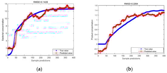
Figure 2.
(a) PCA-PLS model predicts bacterial concentration; (b) PCA-PLS model predicts product concentration.
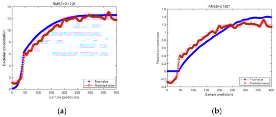
Figure 3.
(a) ICA-PLS model predicts bacterial concentration; (b) ICA-PLS model predicts product concentration.
As can be seen from Figure 2 and Figure 3, for the predicted value of cell concentration and the predicted value of product concentration, after the data are processed by the ICA method, the RMSE values predicted by PLS regression are 0.1296 and 0.1807, respectively. It is lower than the RMSE value predicted by PLS regression after the data are processed by PCA, which are 0.1428 and 0.2264, respectively. It is proved that the ICA-PLS method can effectively separate non-Gaussian data. Its prediction accuracy is stronger than that of the PCA-PLS method.
The same 400 sets of data were processed by the ICA method and then subjected to LWPLS regression and PLS regression, respectively. The LWPLS regression analysis was carried out by setting the location parameter to 0.2 and the number of hidden variables to 4. The results of the two regressions are compared in Figure 4.
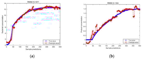
Figure 4.
(a) ICA-LWPLS model predicts bacterial concentration; (b) ICA-LWPLS model predicts product concentration.
It can be seen from the above figure that, for the predicted value of bacterial cell concentration and the predicted value of product concentration, the RMSE values of the LWPLS regression prediction after the data are processed by the ICA method are 0.1071 and 0.1354, respectively, which are lower than the data processed by the ICA before the PLS regression is performed. The predicted RMSE values are 0.1296 and 0.1807, respectively. After proving the LWPLS method, introducing the idea of just-in-time learning, its prediction accuracy is stronger than the traditional PLS method.
The same 400 sets of data are divided into four equal parts and put into four databases of 100 pieces of data each, and the Bayesian classifier is generalized by learning the data from the four databases. When new data are input, the predicted points are first classified into the database of the corresponding stage based on the posterior probability of the Bayesian classifier. Subsequently, the independent elements of the test data were extracted and recombined, based on the ICA algorithm, and the combined data were input into the LWPLS sub-model, with the location parameter, , set to 0.2 and the number of hidden variables set to 4, and locally weighted partial least squares regression was performed. Finally, the predicted values of each LWPLS sub-model were fused with the posterior probabilities obtained from the Bayesian classifier as the weighted coefficients of the subsequent LWPLS sub-models to predict the concentrations of bacteria and products in the products, and the prediction results are shown in Figure 5.
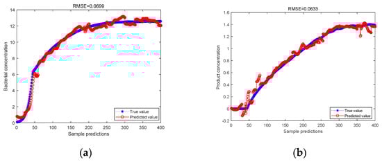
Figure 5.
(a) ICA-JITL-LWPLS model predicts bacterial concentration; (b) ICA-JITL-LWPLS model predicts product concentration.
As can be seen from the above figure, for the predicted value of bacterial cell concentration and the predicted value of product concentration, the data are measured by the Bayesian classifier, and then the RMSE values predicted by LWPLS regression after processing by the ICA method are 0.0699 and 0.0633, respectively. This is lower than the RMSE values of 0.1071 and 0.1354, respectively, which are lower than the RMSE values of LWPLS regression prediction after the data are directly processed by ICA without the similarity measurement of the Bayesian classifier. It is proved that after adding the Bayesian classifier to measure the similarity, the LWPLS method with the idea of instant learning is introduced. Its prediction accuracy is stronger than that of the LWPLS method under the traditional JITL idea.
The above conditions were held constant, and the KICA algorithm based on Gaussian kernel function was used to extract the independent elements of the test data and recombine them. The combined data were input into the LWPLS sub-model to predict the concentrations of bacteria and products in the products, and the predicted results are shown in Figure 6.
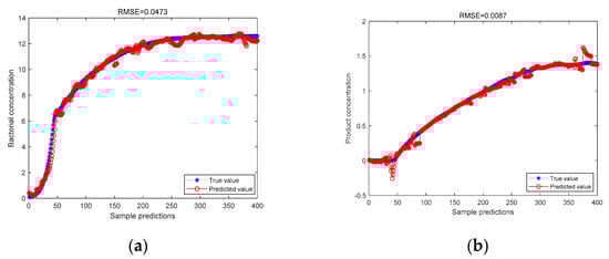
Figure 6.
(a) The KICA-JITL-LWPLS model based on the Gaussian kernel function predicts the bacterial concentration; (b) the KICA-JITL-LWPLS model based on the Gaussian kernel function predicts the product concentration.
As can be seen from the above figure for the predicted values of bacteriophage concentration and product concentration, the RMSE values of 0.0473 and 0.0087 for the data predicted by the Bayesian classifier for similarity metric, followed by the Gaussian kernel function-based KICA algorithm for LWPLS regression prediction, are lower than the RMSE values of 0.0699 and 0.0633 for the data predicted by the Bayesian classifier for similarity metric, followed by the Gaussian kernel ICA for LWPLS regression prediction, respectively. The RMSE values for the LWPLS regression prediction, 0.0699 and 0.0633, respectively, demonstrate that the Gaussian kernel function-based KICA algorithm can better handle non-linear data and improve the prediction accuracy after the similarity measurement by the Bayesian classifier.
The above conditions were held constant, and the KICA algorithm, based on the wavelet kernel function, proposed in this paper was used to extract the independent elements of the test data and recombine them. The combined data were fed into the LWPLS sub-model to predict the concentrations of bacteria and products in the products, and the prediction results are shown in Figure 7.
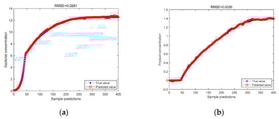
Figure 7.
(a) The KICA-JITL-LWPLS model based on the wavelet kernel function predicts the bacterial concentration; (b) the KICA-JITL-LWPLS model, based on the wavelet kernel function, predicts the product concentration.
As can be seen from the above figure, for the predicted value of cell concentration and the predicted value of product concentration, the data are measured by the Bayesian classifier and then processed by the KICA algorithm, based on the wavelet kernel function, and the RMSE value of the LWPLS regression predictions are made, which are 0.0281 and 0.0036, respectively, which are lower than the RMSE values predicted by LWPLS regression after the Bayesian classifier is used to measure the similarity and processed by the KICA algorithm, based on the Gaussian kernel, which are 0.0473 and 0.0087, respectively. It is proved that the KICA algorithm, based on the wavelet kernel function, proposed in this paper can better deal with non-Gaussian and nonlinear data and improve the prediction accuracy after the Bayesian classifier performs the similarity measurement. The RMSE values of the predicted bacterial concentration and product concentration using the above algorithm are compared in Table 2.
Table 2.
Comparison table of RMSE values of predicted values of cell concentration and product concentration of different models.
R2 reflects the proportion of the total variance of the dependent variable that can be explained by the independent variable through the regression relationship. The closer the R2 metrics is to 1, the higher the fitting degree between the predicted value and the actual value; the comparison of R2 indicators of different models is shown in Table 3.
Table 3.
R2 evaluation metrics.
It can be seen from Table 3 that the R2 metrics of the model proposed in this paper is closer to 1 than the R2 metrics of other models, indicating that the prediction results of the model proposed in this paper are closer to the true value.
In addition, this paper compares the calculation time of each model. The program running timing function of MATLAB is used, and the same set of data is used to record the calculation time of the model proposed in this paper and the calculation time of the other five models. The comparison results are shown in Table 4.
Table 4.
Comparison of calculation time of each model.
It can be seen from Table 4 that although the calculation time of the wavelet kernel KICA-JITL-LWPLS model proposed in this paper is relatively long, it is not much different from the calculation time of the other five models, within 3 s.
5. Conclusions
For the intermittent production process with obvious stage characteristics, this paper proposes a local weighted partial least squares regression quality prediction model, based on the independent element analysis of wavelet kernel function with real-time learning. This model proposes a new wavelet kernel function independent-element analysis method and takes into account the problem that the KICA algorithm based on the wavelet kernel function can process non-Gaussian and nonlinear data but cannot perform regression analysis on the dependent variable, resulting in the inability to perform quality prediction. The quality prediction model based on local weighted partial least squares algorithm based on JITL can perform regression analysis on independent variables and dependent variables at the same time but cannot deal with the problem of inaccurate modeling caused by non-Gaussian and nonlinear data. When new data are input, the model first standardizes the input data and then uses the Bayesian classifier to measure the similarity between the standardized input data and the historical data. Based on the posterior probability of the Bayesian classifier, the subsequent input data are classified into the historical data group with high similarity; the contrast function of the data group is extended to the RKHS space, and the independent element analysis, based on the wavelet kernel function, is carried out to obtain the independent variable group in the probabilistic sense and then solve the problem. The input data represent a non-Gaussian, nonlinear problem. Then, LWPLS regression analysis, based on real-time learning, is performed on the variable group, and the similarity between local input data is calculated according to the similarity measurement method of Euclidean distance. According to the similarity, instruct the sample to assign priority to construct the local model of the current sample, and finally output the local predicted value according to the PLS, and fuse the posterior probability of the Bayesian classifier with the output predicted value to output. Based on the Pensim simulation platform, the proposed multi-model online modeling method based on the wavelet kernel KICA-JITL-LWPLS proposed in this paper was verified and compared with the models of ICA-PLS, ICA-LWPLS, ICA-JITL-LWPLS, KICA-JITL-LWPLS of Gaussian kernel function. The simulation results show that, compared with the traditional model, the model proposed in this paper can achieve an accurate prediction of bacterial concentration and penicillin concentration, and the RMSE values are reduced by 0.1147 and 0.2228, respectively. It is proved that the method in this paper has a higher prediction accuracy and generalization ability and has a certain reference value for the dynamic modeling research of the batch production process with obvious stage characteristics.
Author Contributions
Conceptualization, L.S. and M.Y.; methodology, L.S.; software, Y.H.; validation, L.S., M.Y. and Y.H.; writing—review and editing, L.S. and M.Y.; supervision, Y.H.; project administration, L.S. and M.Y.; All authors have read and agreed to the published version of the manuscript.
Funding
This work was partially supported by the Youth Innovation Promotion Association CAS (2021203).
Institutional Review Board Statement
Not applicable.
Informed Consent Statement
Not applicable.
Data Availability Statement
Not applicable.
Conflicts of Interest
The authors declare no conflict of interest.
References
- Sanchez-Martos, F.; Jimenez-Espinosa, R.; Pulido-Bosch, A. Mapping groundwater quality variables using PCA and geostatistics: A case study of Bajo Andarax, southeastern Spain. Hydrol. Sci. J. 2001, 46, 227–242. [Google Scholar] [CrossRef]
- Amdevyren, H.; Demyr, N.; Kanik, A.; Keskýn, S. Use of principal component scores in multiple linear regression models for prediction of Chlorophyll-a in reservoirs. Ecol. Model. 2005, 181, 581–589. [Google Scholar] [CrossRef]
- Depczynski, U.; Frost, V.J.; Molt, K. Genetic algorithms applied to the selection of factors in principal component regression. Anal. Chim. Acta 2000, 420, 217–227. [Google Scholar] [CrossRef]
- Wehrens, R.; Linden, W. Bootstrapping principal component regression models. J. Chemom. 2015, 11, 157–171. [Google Scholar] [CrossRef]
- Assent, I. Clustering high dimensional data. Wiley Interdiscip. Rev. Data Min. Knowl. Discov. 2012, 2, 340–350. [Google Scholar] [CrossRef]
- Delorme, A.; Makeig, S. EEGLAB: An open source toolbox for analysis of single-trial EEG dynamics including independent component analysis. J. Neurosci. Methods 2004, 134, 9–21. [Google Scholar] [CrossRef]
- Calhoun, V.D.; Adali, T.; Pearlson, G.D.; Pekar, J. A method for making group inferences from functional MRI data using independent component analysis. Hum. Brain Mapp. 2010, 14, 140. [Google Scholar] [CrossRef]
- Shi, Z.; Tang, H.; Tang, Y. A new fixed-point algorithm for independent component analysis. Neurocomputing 2004, 56, 467–473. [Google Scholar] [CrossRef]
- Bingham, E.; HyvRinen, A. A Fast Fixed-Point Algorithm for Independent Component Analysis. Int. J. Neural Syst. 2000, 10, 1–8. [Google Scholar] [CrossRef]
- Bartlett, M.S.; Movellan, J.R.; Sejnowski, T.J. Face Recognition by Independent Component Analysis. IEEE Trans. Neural Netw. 2002, 13, 1450–1464. [Google Scholar] [CrossRef]
- Delorme, A.; Sejnowski, T.; Makeig, S. Enhanced detection of artifacts in EEG data using higher-order statistics and independent component analysis. Neuroimage 2007, 34, 1443–1449. [Google Scholar] [CrossRef] [PubMed]
- Zhang, Y.; Qin, S.J. Fault Detection of Nonlinear Processes Using Multiway Kernel Independent Component Analysis. Ind. Eng. Chem. Res. 2007, 46, 7780–7787. [Google Scholar] [CrossRef]
- Zhao, C.; Gao, F.; Wang, F. Nonlinear Batch Process Monitoring Using Phase-Based Kernel-Independent Component Analysis Principal Component Analysis (KICAPCA). Ind. Eng. Chem. Res. 2009, 48, 9163–9174. [Google Scholar] [CrossRef]
- Maino, D.; Farusi, A.; Baccigalupi, C.; Perrotta, F.; Banday, A.J.; Bedini, L.; Burigana, C.; De Zotti, G.; Górski, K.M.; Salerno, E. All-sky astrophysical component separation with Fast Independent Component Analysis (FASTICA). Mon. Not. R. Astron. Soc. 2002, 334, 53–68. [Google Scholar] [CrossRef]
- Wang, G.; Hou, Z.; Tang, Y.; Zhao, J.; Sun, Y.; Dong, C.; Fu, D. Determination of endpoint of procedure for radix rehmanniae steamed based on ultraviolet spectrophotometry combination with continuous wavelet transform and kernel independent component analysis. Anal. Chim. Acta 2010, 679, 43–48. [Google Scholar] [CrossRef]
- Zhou, S.K.; Chellappa, R. From sample similarity to ensemble similarity: Probabilistic distance measures in reproducing kernel hilbert space. IEEE Trans. Pattern Anal. Mach. Intell. 2006, 28, 917–929. [Google Scholar] [CrossRef]
- Zhang, Y.; Chi, M. Decentralized fault diagnosis using multiblock kernel independent component analysis. Chem. Eng. Res. Des. 2012, 90, 667–676. [Google Scholar] [CrossRef]
- Gallego-Castillo, C.; Bessa, R.; Cavalcante, L.; Lopez-Garcia, O. On-line quantile regression in the RKHS (Reproducing Kernel Hilbert Space) for operational probabilistic forecasting of wind power. Energy 2016, 113, 355–365. [Google Scholar] [CrossRef]
- Zhang, Z.; Jie, Y.U.; Yan, Q.; Zhao, Z. Research on Polarimetric SAR Image Speckle Reduction Using Kernel Independent Component Analysis. Acta Geod. Cartogr. Sin. 2011, 40, 289–295. [Google Scholar]
- Wang, J.; Shi, Q. Short-term traffic speed forecasting hybrid model based on chaos–wavelet analysis-support vector machine theory. Transp. Res. Part C Emerg. Technol. 2013, 27, 219–232. [Google Scholar] [CrossRef]
- Kaneko, H.; Funatsu, K. Ensemble locally weighted partial least squares as a just-in-time modeling method. AIChE J. 2016, 62, 717–725. [Google Scholar] [CrossRef]
- Antoniadis, A.; Paparoditis, E.; Sapatinas, T. A functional wavelet–kernel approach for time series prediction. J. R. Stat. Soc. Ser. B (Stat. Methodol.) 2006, 68, 837–857. [Google Scholar] [CrossRef]
- Bowen, H.P.; Wiersema, M.F. Modeling limited dependent variables: Methods and guidelines for researchers in strategic management. In Research Methodology in Strategy and Management; Emerald Group Publishing Limited: Bingley, UK, 2004; Volume 1, pp. 87–134. [Google Scholar]
- Wang, G.; Hou, Z.; Peng, Y.; Wang, Y.; Sun, X.; Sun, Y.-A. Adaptive kernel independent component analysis and UV spectrometry applied to characterize the procedure for processing prepared rhubarb roots. Analyst 2011, 136, 4552–4557. [Google Scholar] [CrossRef] [PubMed]
- Rashid, M.M.; Yu, J. Nonlinear and Non-Gaussian Dynamic Batch Process Monitoring Using a New Multiway Kernel Independent Component Analysis and Multidimensional Mutual Information Based Dissimilarity Approach. Ind. Eng. Chem. Res. 2012, 51, 10910–10920. [Google Scholar] [CrossRef]
- Wehrens, R.; Mevik, B.H. The pls Package: Principal Component and Partial Least Squares Regression in R. J. Stat. Softw. 2007, 18, 1–24. [Google Scholar]
- Carrascal, L.M.; IGalván Gordo, O. Partial least squares regression as an alternative to current regression methods used in ecology. Oikos 2010, 118, 681–690. [Google Scholar] [CrossRef]
- Abdi, H. Partial least squares regression and projection on latent structure regression (PLS-regression). Wiley Interdiscip. Rev. Comput. Stat. 2010, 2, 97–106. [Google Scholar] [CrossRef]
- Helander, E.; Virtanen, T.; Nurminen, J.; Gabbouj, M. Voice Conversion Using Partial Least Squares Regression. IEEE Trans. Audio Speech Lang. Processing 2010, 18, 912–921. [Google Scholar] [CrossRef]
- Bevilacqua, M.; Marini, F. Local classification: Locally weighted-partial least squares-discriminant analysis (LW-PLS-DA). Anal. Chim. Acta 2014, 838, 20–30. [Google Scholar] [CrossRef]
- Hazama, K.; Kano, M. Covariance-based locally weighted partial least squares for high-performance adaptive modeling. Chemom. Intell. Lab. Syst. 2015, 146, 55–62. [Google Scholar] [CrossRef]
- Okajima, T.; Kim, S. Selection of Similarity Measure for Locally Weighted Partial Least Squares Regression. In Proceedings of the 2011 AIChE Annual Meeting, Minneapolis, MN, USA, 16–21 October 2011. [Google Scholar]
- Yoshizaki, R.; Kano, M.; Kim, S. Optimization of nonlinear multi-stage process with characteristic changes through locally-weighted partial least squares. In Proceedings of the 2015 10th Asian Control Conference (ASCC), Kota Kinabalu, Malaysia, 31 May 2015–3 June 2015. [Google Scholar]
- Yeo, W.S.; Saptoro, A.; Kumar, P. Development of Adaptive Soft Sensor Using Locally Weighted Kernel Partial Least Square Model. Chem. Prod. Process Modeling 2017, 12, 22. [Google Scholar] [CrossRef]
- Xiong, W.; Xue, M.; Li, Y. Online Modeling with Semi-Supervised Locally Weighted Partial Least Squares Based on Expectation Maximization Algorithm. J. Syst. Simul. 2018, 30, 8–10. [Google Scholar] [CrossRef]
- Qi, S.; Yan, Y.; Jinhui, C.; Yingying, Z. Proximate Analysis of Sawdust Using Near Infrared Spectroscopy and Locally Weighted Partial Least Squares. Energy Procedia 2016, 88, 600–607. [Google Scholar] [CrossRef][Green Version]
- Thébault, A.; Juery, D. Locally-Weighted Partial Least Squares Regressionfor Infrared Spectra Analysis. In Proceedings of the 1ères Rencontres R; Hal, Bordeaux, France, 2 July 2012. [Google Scholar]
- Song, Y.; Ren, M. A Novel Just-in-Time Learning Strategy for Soft Sensing with Improved Similarity Measure Based on Mutual Information and PLS. Sensors 2020, 20, 3804. [Google Scholar] [CrossRef] [PubMed]
- Cheeseman, P.; Kelly, J.; Self, M.; Stutz, J.; Taylor, W.; Freeman, D. Autoclass: A Bayesian classification system. In Proceedings of the Fifth International Conference on Machine Learning, Ann Arbor, MI, USA, 12–14 June 1988; pp. 54–64. [Google Scholar]
- Jahani, M.; He, X.; Ma, C.; Mokhtari, A.; Mudigere, D.; Ribeiro, A.; Takac, M. Efficient distributed hessian free algorithm for large-scale empirical risk minimization via accumulating sample strategy. In Proceedings of the International Conference on Artificial Intelligence and Statistics, Online, 26–28 August 2020; pp. 2634–2644. [Google Scholar]
- Serwecińska, L. Antimicrobials and antibiotic-resistant bacteria: A risk to the environment and to public health. Water 2020, 12, 3313. [Google Scholar] [CrossRef]
- Börsch-Supan, A.; Ludwig, A.; Winter, J. Ageing, Pension Reform and Capital Flows: A Multi-Country Simulation Model. Economica 2006, 73, 625–658. [Google Scholar] [CrossRef]
- Birol, G.; Ündey, C.; Cinar, A. A modular simulation package for fed-batch fermentation: Penicillin production. Comput. Chem. Eng. 2002, 26, 1553–1565. [Google Scholar] [CrossRef]
Publisher’s Note: MDPI stays neutral with regard to jurisdictional claims in published maps and institutional affiliations. |
© 2022 by the authors. Licensee MDPI, Basel, Switzerland. This article is an open access article distributed under the terms and conditions of the Creative Commons Attribution (CC BY) license (https://creativecommons.org/licenses/by/4.0/).