Abstract
With the continuous improvement of industrial production requirements, bearings work significantly under strong noise interference, which makes it difficult to extract fault features. Deep Learning-based approaches are promising for bearing diagnosis. They can extract fault information efficiently and conduct accurate diagnosis. However, the structure of deep learning is often determined by trial and error, which is time-consuming and lacks theoretical support. To address the above problems, an adaptive (Adaptive Depthwise Separable Dilated Convolution and multi-grained cascade forest) ADSD-gcForest fault diagnosis model is proposed in this paper. Multiscale convolution combined with convolutional attention mechanism (CBAM) concentrates on effectively extracting fault information under strong noise, and the Meta-Activate or Not (Meta-ACON) activation function is integrated to adaptively optimize the model structure according to the characteristics of input samples, then gcForest outputs the final diagnosis result as the classifier. The experiment compares the effects of three bearings failure diagnoses under various noise and load conditions. The experimental results show the effectiveness and practicability of the proposed method.
1. Introduction
With the development of the manufacturing industry, rolling bearings, as one of the core components of mechanical equipment, play an increasingly irreplaceable role. However, under the condition of strong noise and multiple loads for a long time, the bearings are prone to wear or breakage. An expected failure, such as a crack in the bearings, may cause the breakdown of the entire machine, resulting in magnificent economic loss and severe safety accidents [1]. Therefore, it is of great significance to realize the high efficiency and accuracy of bearing fault diagnosis.
The location of the bearing failure is generally located in the inner ring, outer ring, and rolling element, and the bearing fault usually produces periodic vibrations when machinery is running, so analysis of the vibration signal during bearing operation is the key to achieving the diagnosis of the fault [2]. Traditional fault diagnosis methods are divided mainly into linear and non-linear methods. Linear diagnosis methods mainly contain time domain analysis, frequency domain analysis, and time-frequency analysis [3]. Nonlinear analysis is less adopted in fault diagnosis than linear analysis, chaos theory, fractal dimension, and entropy value theory, are commonly applied nonlinear analysis methods, among others. However, due to the increase in bearing fault datasets and the increasing complexity of production environments, traditional fault diagnosis methods that rely on traditional manual fault sign extraction have become no longer applicable [4]. Therefore, constructing novel fault diagnosis models based on approaches of deep learning have become a research hotspot.
Frequently used deep learning models include the Deep Autoencoder (DAE), the Deep Belief Network (DBN), the Convolutional Neural Network (CNN) and the Recurrent Neural Network (RNN). Among them, the improved Stack Denoising Autoencoder (SDAE) diagnostic method was proposed by Hou et al. [5], in which the hyperparameters of the DAE network were adaptively selected by the particle swarm algorithm to determine the structure of the SDAE network. On this basis, the characteristic representation of the fault state was obtained, which was input into the Softmax classifier for fault classification and recognition; this method has achieved accurate fault diagnosis under the circumstance of variable operating conditions. In-depth research on DAE was conducted by Shao et al. [6], in which DAE and shrinking auto-encoding were introduced to improve the fault extraction capabilities of faulty features, and local preservation of projection fusion features was applied to optimize feature quality. Liang T et al. [7] presented a method for the diagnosis of rolling bearing failures, which consisted mainly of three steps: a series of DBNs with different hyperparameters were constructed and trained, after which the improved ensemble method was applied to acquire the weight matrix for each DBN and then each DBN voted together according to its respective weight matrix to obtain the final result of the diagnosis. The method of DBN-based degradation assessment under accelerated life testing of bearings was adopted by Ma et al. [8]. Shao et al. proposed a DBN for the diagnosis of induction motors faults, in which vibration signals were introduced directly as input [9], and the t-SNE algorithm was adopted to visualize the learning representation. Han Tao et al. [10] used CNN training to obtain the corresponding characteristic diagram of the multi-wavelet coefficient branching process through the wavelet transform to realize the intelligent diagnosis of rolling bearing composite faults. Liang et al. [11] have constructed two different CNNs, one for extracting time-domain features and the other was applied to extract time-frequency domain features, and then fused them with the time-frequency features and time-domain features extracted by continuous wavelet transform diagnose faults of rolling bearings in a characteristic way. Bearing fault diagnosis based on LSTM (Long Short-Term Network) and CNN models was established by Pan et al. [12], a fault diagnosis method was proposed by Zhang et al. [13], in which self-encoding of convolutional noise reduction was performed to achieve feature extraction and CNN was introduced for pattern recognition. The long- and short-term memory stacking network was designed by Yu et al. [14], where 12 different bearing health conditions were classified using augmented data, including the type and severity of bearing failure. A convolutional bidirectional long- and short-term memory network was designed by Zhao et al. [15] for bearing fault diagnosis. In this method, a convolutional neural network was applied as a feature extractor of the original signal, and then the bearing faults were classified through a bidirectional long and short-term memory network.
Based on the brief review of the existing diagnosis approaches, the challenges can be summarized as follows: first of all, numerous methods only conduct comparative experiments for a single type of noise and other types of noise are not considered. Second, deep learning structures are often determined by trial and error, which means this structure is randomly defined; as a result, the model with the best performance is adopted after many experiments [16]. To solve the above problem, an adaptive ADSD-gcForest fault diagnosis model is proposed in this paper, and based on the basis of the existing traditional network, the core fault features at different scales are effectively extracted by using dilated convolution with different dilation rates and CBAM fusion under strong noise interference. On this basis, deep separable convolution is incorporated into the dilated convolution mechanism to improve the efficiency of the calculation [17]. In recent years, many adaptive optimization methods have been developed for network structure, but most of these approaches require the assistant of an intelligent optimization algorithm or migration learning [18,19]. In contrast, the network structure can be simply optimized by the Meta-ACON activation based on the input samples without the need for additional complex algorithms and can not only optimize the model structure but also make the model better deal with different sample data. Then, through the multigranular scanning of the deep forest classifier and the cascade forest algorithm, the hidden fault features in the feature vector are analyzed and extracted, and the final classification results are output. The main contributions of this article are as follows:
- An adaptive ADSD-gcForest diagnostic model is proposed for the diagnosis of rolling bearing fault diagnosis, allowing the extraction of features under the high-noise and complex working conditions that could be realized. The structure of the diagnosis model achieves adaptive optimization based on the characteristics of the sample data.
- Combining the multiscale depth-separable dilated convolution with CBAM can effectively extract fault features under strong noise interference. On the basis of the lack of adjust the original structure of the model, the Meta-ACON activation function is introduced into the convolution layer of the model to achieve adaptive optimization of the model structure according to the fault data of different bearings.
- The comparative experiment shows that the ADSD-gcForest model proposed in this paper has strong generalization ability and robustness with certain practical value.
2. Related Works
2.1. SDP Image
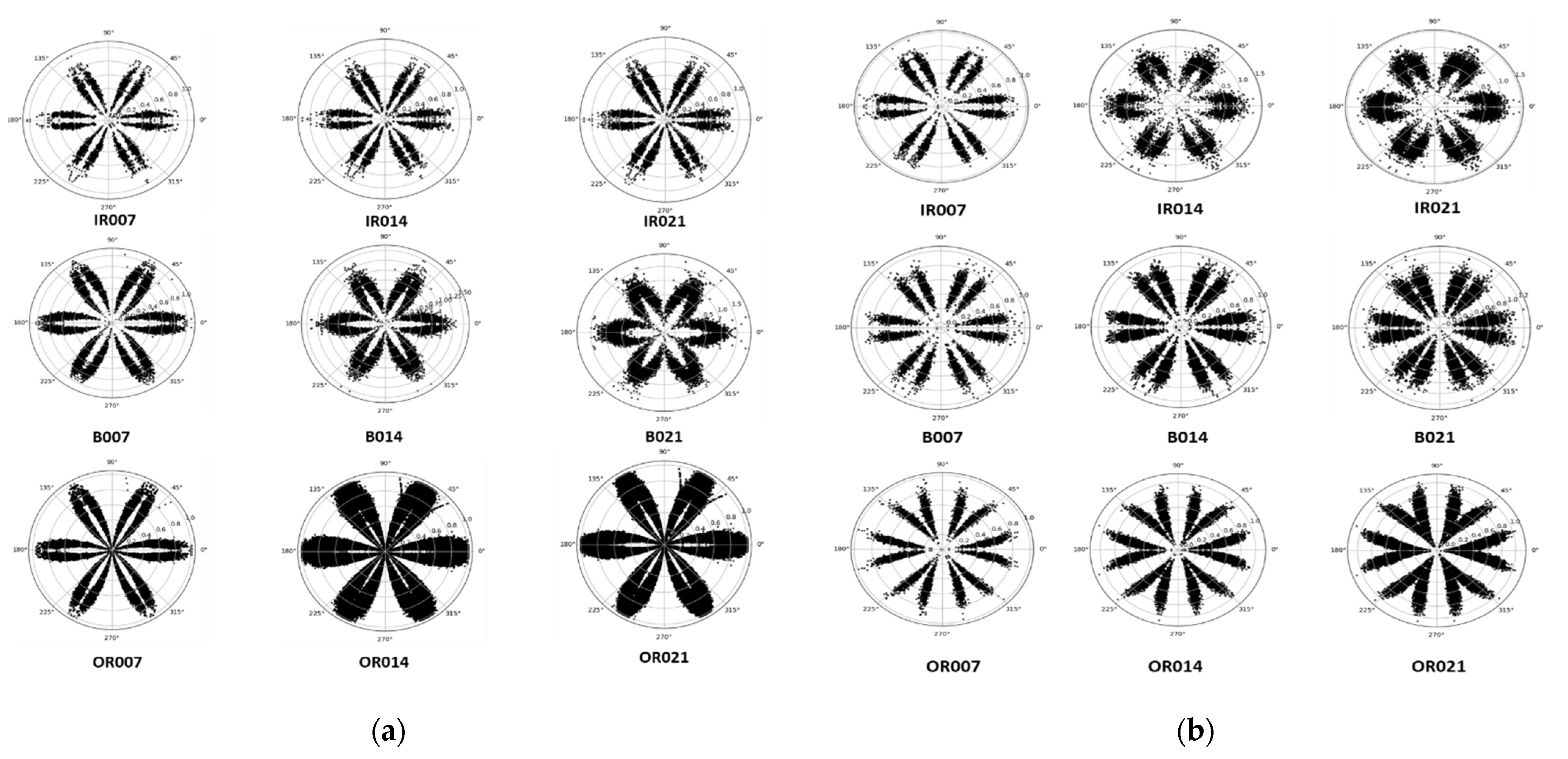
Through the normalization method, the time domain signal can be described in the polar coordinate system. Thus, the vibration signal can be converted to SDP images [20], and the relationship between the amplitude and the frequency of the vibration signal can be described simply and directly through the geometric shape. The specific mapping relationship is as follows:
where the input vibration signal is represented as , i represents the sequence number of the discrete sampling point of the signal in the time domain, the maximum and minimum values of the vibration signal are, respectively, described as and and the amplitude of corresponding to the time lag coefficient a is shown as , the radius of the polar coordinates is indicated as r(i), δ is the magnification angle, is the angle of the l-th mirror symmetry plane, θ(i) and φ(i) are the deflection angles of the mirror symmetry plane, where δ ≤ and (l ∈ (0, N−1)), and N is the number of symmetry planes. SDP images of different fault characteristics will present various geometric characteristics, which are manifested mainly in the curvature, thickness, geometric center and concentrated area of the image arm of the SDP image [21]. The SDP images of different fault characteristics are shown in Figure 1. Among them, IR, OR and B, respectively, represent the inner ring, outer ring and rolling element, while 007, 014, and 021 indicate that the fault diameter is 0.1778 mm, 0.3556 mm and 0.5334 mm separately.

Figure 1.
SDP images. (a) Drive end bearing, (b) Fan end bearing.
2.2. Dilated Convolutional
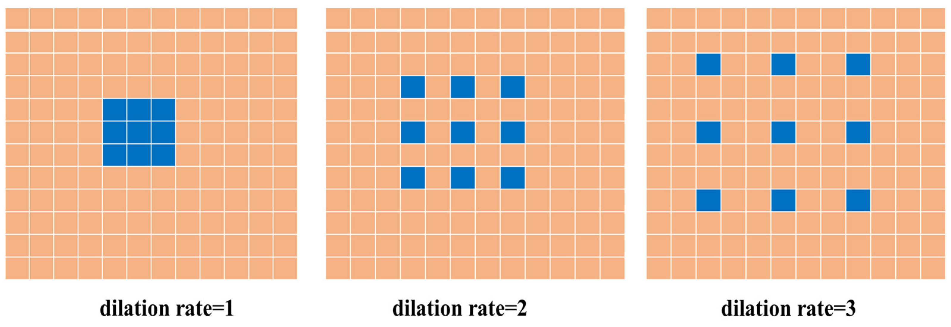
Unlike ordinary convolution, the dilated convolution is one of the convolutional neural networks which increases the receptive field of the output unit without increasing the parameters, which is mainly implemented by introducing the dilation rate parameter. Specifically, it mainly depends on the way of interval sampling, which means that the spacing of each value is defined by the dilation rate when the convolution kernel processes the data. Thus, the receptive field can be increased without reducing the image resolution. For convolution kernels of the same size, the larger the dilation rate, the greater the receptive field of the convolution kernel [22]. The calculation formula for the receptive field of the dilated convolution is as follows:
where the receptive field of the current layer is presented as rn, is the upper receptive field and k is the size of the convolution kernel. The sampling process is shown in Figure 2.

Figure 2.
Dilated convolution.
2.3. Depth-Separable Convolution
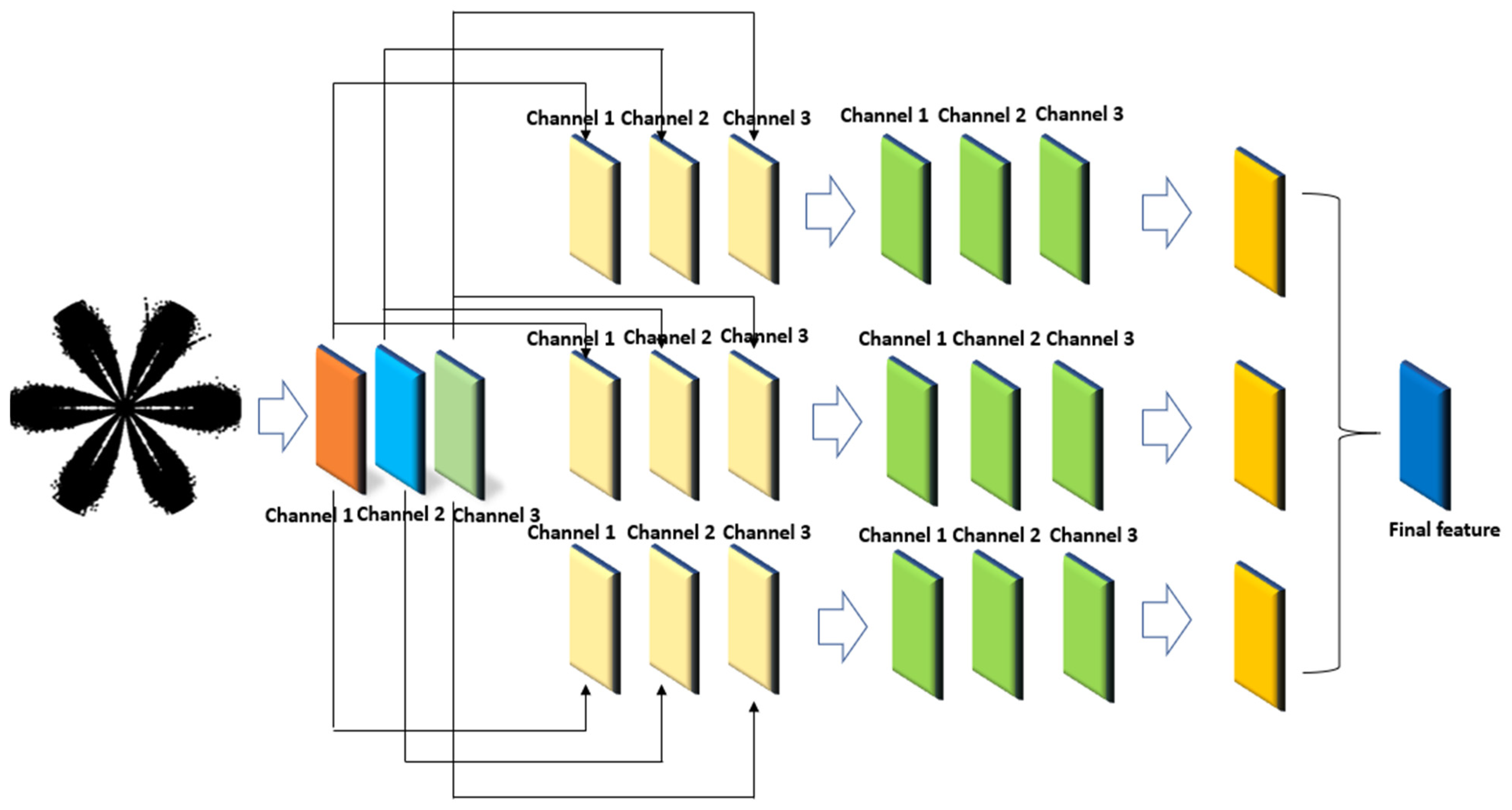
The standard convolution is decomposed into deep convolution and point-wise convolution by depth-separable convolution [23,24,25]. First, each channel of the input sample is convolved one by one by the deep convolution; thus, the number of feature maps generated is the same as the number of channels of the input sample, and after that, the feature map is reconstructed with weights which are assigned on the basis of the designed algorithm according to point-by-point convolution. In this way, the amount of calculation and parameters of the model can be reduced in both time and space. For example, the dimension of the input samples is set as , the output dimension is arranged accordingly as and the sizes of the convolution kernel are , where are the number of channels. The formula to calculate the total number of parameters for ordinary convolution and deeply separable convolution is shown in Formulas (5) and (6), respectively, where represents the total number of parameters for ordinary convolution and the total number of parameters for deeply separable convolution is . The specific schematic diagram is shown in Figure 3, where channel 1, channel 2 and channel 3, respectively, indicate the three dimensions of the input image.
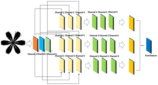
Figure 3.
Depth-separable convolution.
2.4. CBAM
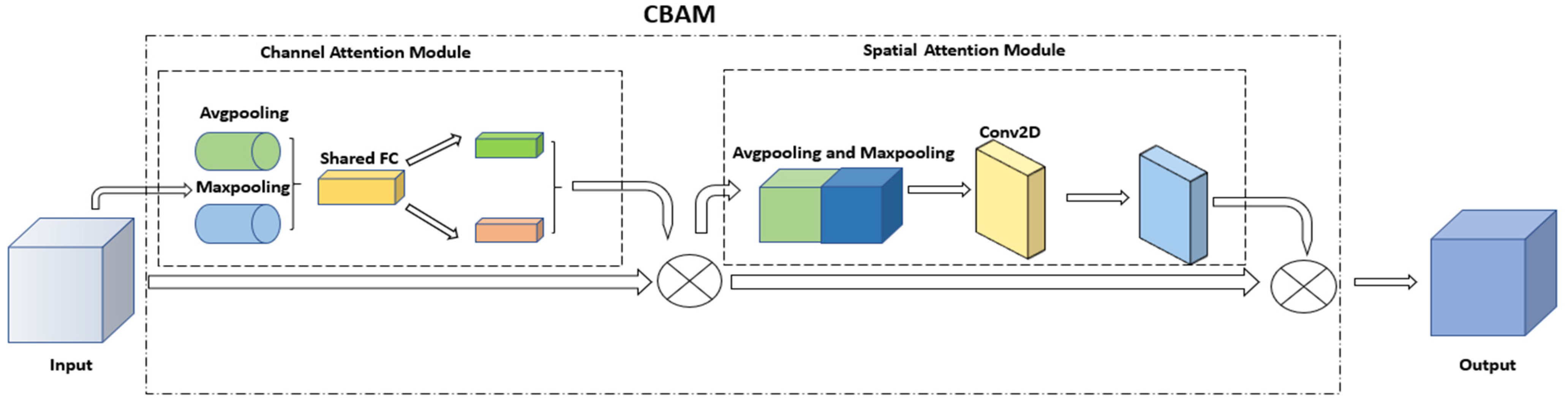
The attention mechanism is derived from the human visual mechanism, which is widely used in image processing. CBAM has been widely used in target detection by skillfully integrating spatial attention mechanism and channel attention mechanism [26,27,28]. Primarily, the channel attention mechanism selects which features are the key features, and then uses the spatial attention mechanism to learn the location of the key features, strengthening the extraction of the core features of the input sample; from this, in addition, the model can achieve adaptive refinement of the core features in the images. The specific composition structure is shown in Figure 4, where Avgpooling and Maxpooling, respectively, represent the average pooling and maximum pooling, while shared FC means the shared full connectivity layer.
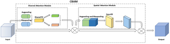
Figure 4.
CBAM.
2.5. gcForest
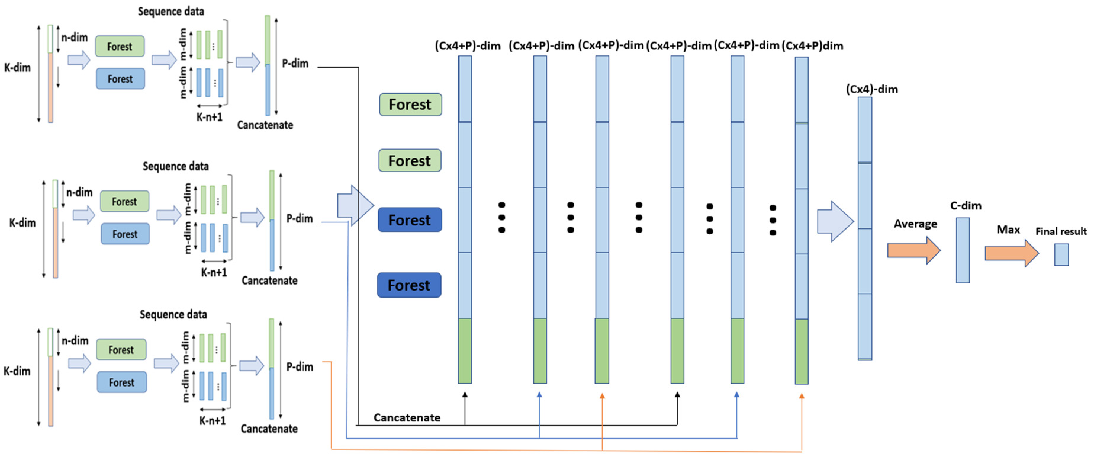
Different from the traditional Softmax classifier, the hidden features of the input feature vector can be learned by gcForest through the superposition of multi-layer random forests, which then output the final classification results [29,30]. It has been proven that the accuracy of the deep forest classifier is about 1–4% higher than that of the Softmax classifier. The deep forest classifier mainly consists of two parts: multi-granularity scanning and cascade forest. The feature vector is sampled in a sliding window to form a new feature vector, which will be input into the cascade forest. After passing through the multi-layer random forest, the final output class probability distribution vector is taken as the final classification result. The specific structure of the deep forest classifier is shown in Figure 5, where K is the dimension of the input vector table type, n is the dimension of the sliding window, m as the category of the classification number and P is the final output vector whose dimension. Furthermore, in Figure 5, the scanned vector is input into the cascade forest, the blue and green two color Forests, respectively, represent random forest and completely random forest, each layer contains two random forests and two completely random forests and each forest after the completion of a training will be an output vector, of which the dimension is C. The output vectors of the four forests are stacked with the output vectors of multi-granularity scanning, and the vector with dimension (C × 4 + P) is the output; moreover, after multi-layer learning, the output vectors of the last layer are averaged to obtain the final probability category vector with dimension C and the maximum probability of the vector is taken as the classification result.

Figure 5.
gcForest.
3. Method
The ADSD-gcForest model will be described in detail in this section. The detailed implementations of the method are described in the following three steps.
Step 1: A sliding window is used to sample vibration signals, then the noise of different intensity is added and the signals are converted into SDP image, and then the sample data are divided into a training set and a test set.
Step 2: The training set is entered into the adaptive ADSD-gcForest model for training and the Meta-ACON activation function is applied to adaptively adjust the network structure, according to different types of sample data to obtain the current optimal model structure, after which the trained model is saved.
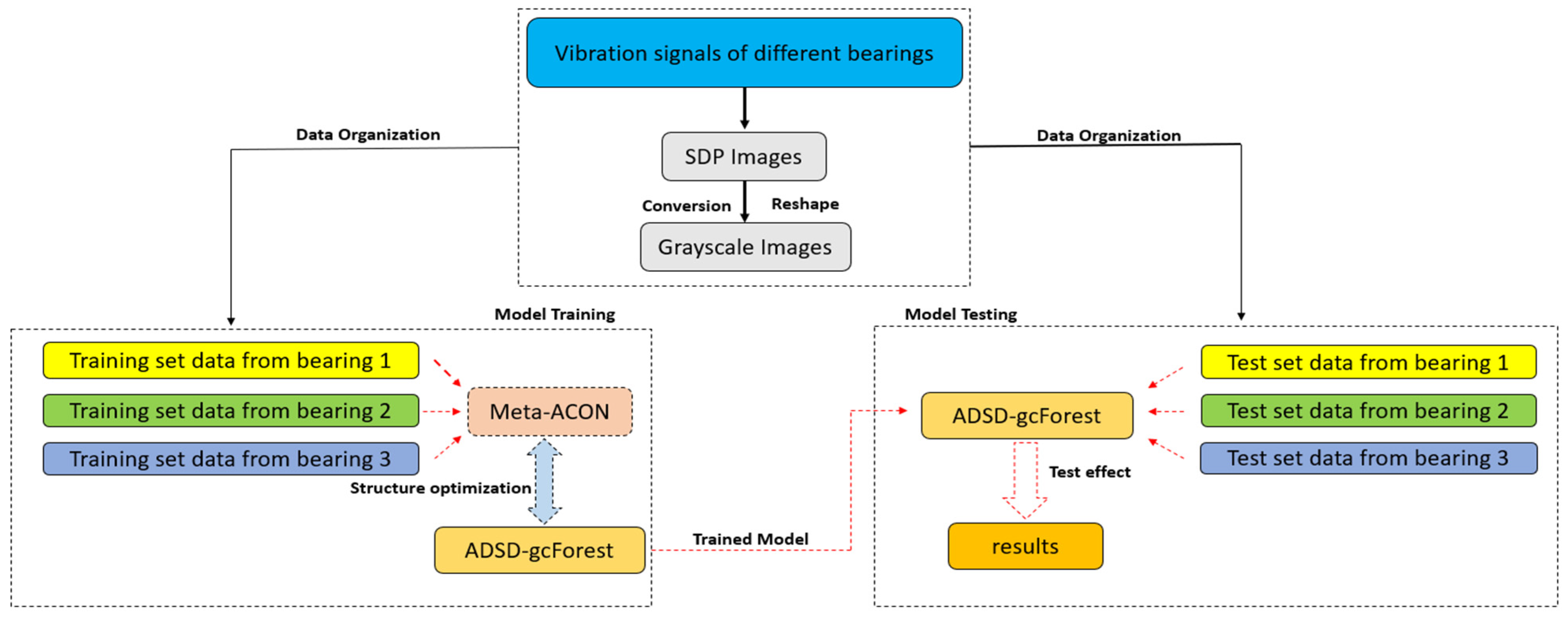
Step 3: The trained model is used to directly extract fault features from new images, which results in the final diagnosis. The overall flowchart of the fault diagnosis is drawn in Figure 6.
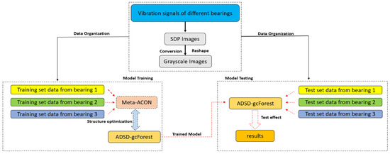
Figure 6.
The overall flowchart of the fault diagnosis.
3.1. Meta-ACON
In order to achieve more effective fault diagnosis based on different bearing fault data, it may be necessary to continuously adjust the existing structure to achieve higher accuracy. In order to solve the above problems, a relatively simple way to achieve adaptive adjustment of the network model is proposed in this paper: by setting a single conversion factor β, the Meta-ACON activation function can simply select whether to activate the neurons in this layer according to different sample data (activation represents nonlinear output, while on the contrary, non-activation represents linear output). The design of the Meta-ACON activation function is derived from the smooth maximum function, and its formula is as follows:
where represents the input signal sequence, is the conversion factor, when →∞, →max and →0, and is the arithmetic mean value. Many common activation functions have the form max (ηa (x), ηb (x)). ηa (x) and ηb (x) are two freely configurable functions. For example, in the ReLU function, ηa (x) = x and ηb (x) = 0, many activation functions can be expressed in the form of max (ηa (x), ηb (x)). To simplify the design, only two variables are considered here, and the sigmoid function is simplified as σ. At this time, the approximate relationship is represented as:
Furthermore, = , = and ≠ . The Meta-ACON activation function is as follows:
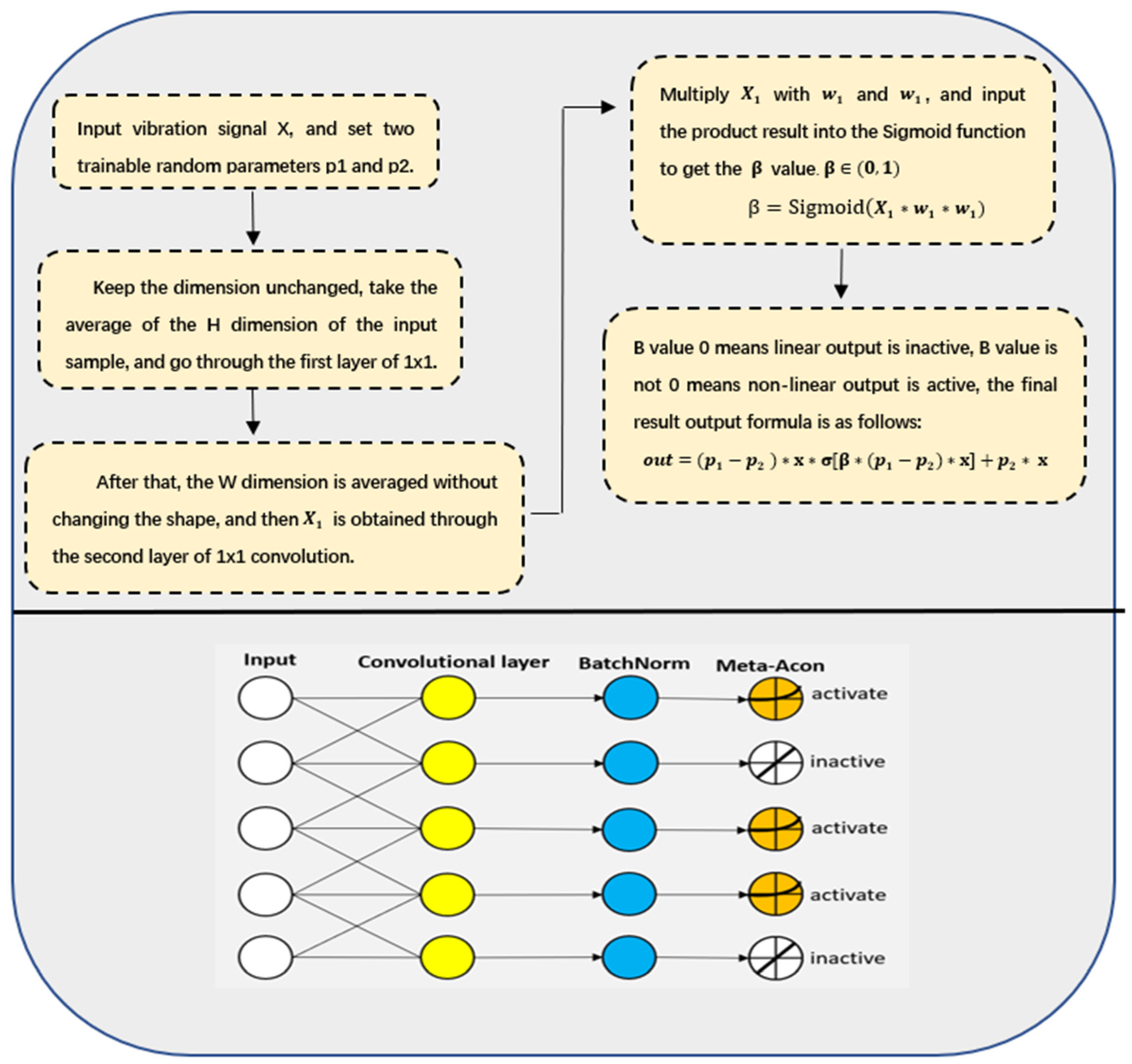
Among them, and are two random trainable parameters; therefore, the activation of neurons in this layer can be easily controlled by means of conversion factor , where , the input sample data is represented as and c, h and w, respectively, describe the number of channels, width and height of the input sample data. is the convolution of the sample data with the number of input channels as the width of the sample, the number of output channels as the width/r (r is a constant, generally taken as 16) and the convolution core size of 1 × 1. Similarly, is also obtained by the convolution with the convolution core size of 1 × 1, except that the number of output channels and input channels of convolution are opposite to the setting of . Since the value is directly determined by the structural characteristics of the sample data, different sample data will produce different values, Therefore, after many times of training, with the continuous updating of Meta-ACON parameters, the structure of the model can be continuously optimized. The specific calculation process is shown in Figure 7.

Figure 7.
The specific calculation process of Meta-ACON.
3.2. ADSD-gcForest
Compared with time-domain signals, SDP images can represent different fault types in a more intuitive and simple way by presenting different geometric features. Therefore, the key to achieve an accurate fault diagnosis is to design a diagnosis model that can effectively extract geometric features from images. The visual geometry group 16 (VGG16) is one of the commonly used models in image processing. Feature extraction is effectively realized by stacking multilayer convolution, and network parameters are reduced by pooling layer. The model in this paper takes VGG16 as the basic framework. However, the structure of VGG16 network is relatively simple. Firstly, although the network is deep, ordinary convolution is widely used in convolution layers, which cannot extract the sample feature information in multiple scales, which limits the feature extraction ability of the network under the intervention of strong noise. Second, most of the activation functions in the convolution layer simply make the input signal become non-linear, so the network does not have good migration learning ability; thus, in the face of different sample data, the performance of the network will become unstable. Moreover, most diagnostic models use Softmax as the final classifier, However, Softmax is not an advanced classifier and cannot learn the feature information that has not been extracted, so as to reduce the final accuracy. In response to the above problems, the ADSD-gcForest model proposed in this paper makes the following improvements.
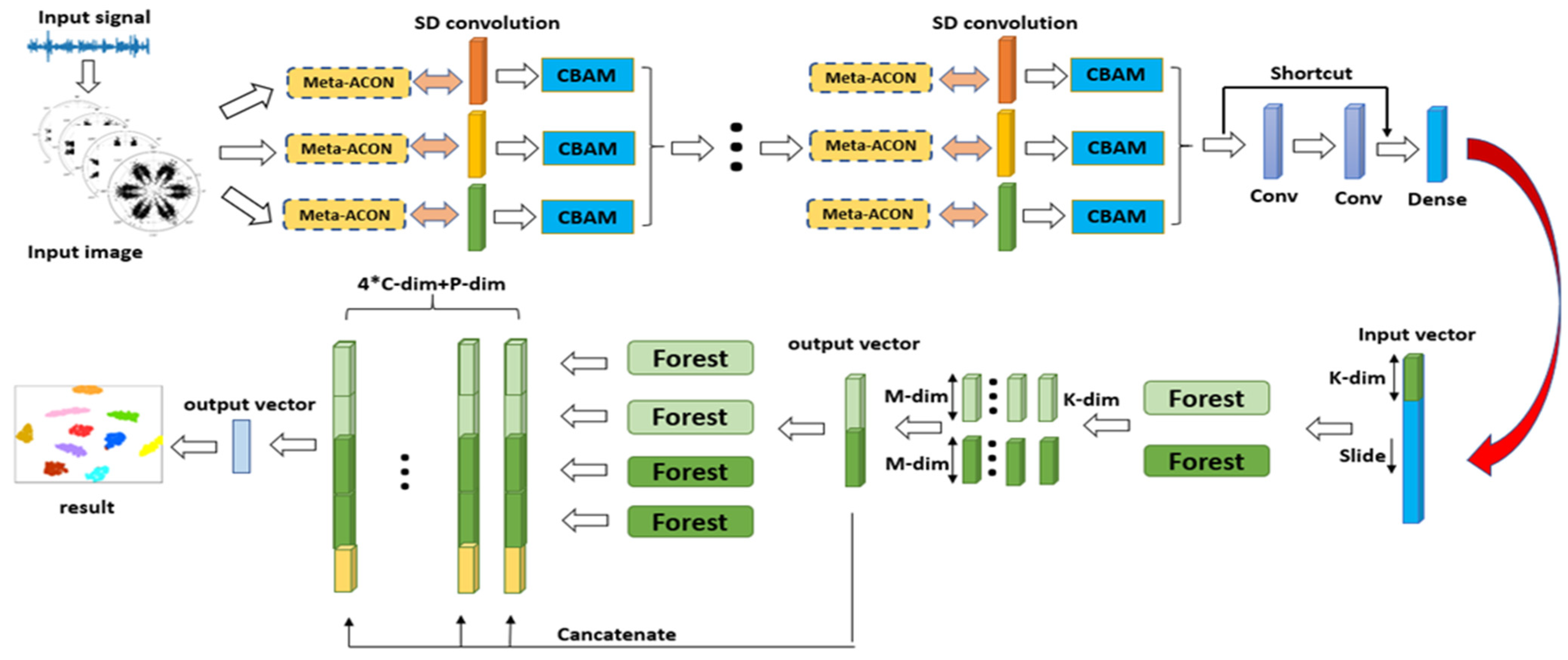
Due to the large number of input sample types, in order to increase the model feature extraction range and enrich the feature information, the characteristics of the receptive field are expanded by using the dilated convolution and combined with the residual network to build three branches. Therefore, the construction of three kinds of dilated convolutions with different dilation rates is connected through the residual network, the dilation rate is set to 1, 2 and 3 and the size of the convolution kernel is 3 × 3. Thus, multi-scale feature extraction is realized. After the dilated convolution with different expansion rates, it is combined with the CBAM, and the channel attention mechanism is used to measure the importance of different kinds of channel feature information in the feature map at different scales, so as to determine the key points under different channels in the feature map features. Then, the spatial attention mechanism is introduced to locate these key features and extract the key feature information from the feature map to obtain key features at different scales. Next, three feature maps are obtained and integrated using the residual network and input into the next layer. Due to the use of more dilated convolution and attention mechanisms in the network, it may lead to a longer network training time. Since the convolution operations for different channels of the input image can be simultaneously performed by the depth-separable convolution, the depth-separable convolution mechanism is led into the dilated convolution layer, after which the weight ratio of each feature map is determined through quasi-point convolution, and the the feature maps are integrated according to the weights. Thus, computational efficiency could be improved in this way. In order to realize that the network model can be adaptively adjusted according to the sample data of different fault types, the original ReLU activation function in the convolutional layer is replaced with the Meta-ACON activation function. The Meta-ACON activation function can be based on the size characteristics of the input image. By setting the conversion factor β, the value of β determines whether to activate the neurons in this layer after multiple trainings, and a flexible and efficient network structure can be adopted for the training model according to different input samples. Softmax is replaced by gcForest, which learns the hidden fault characteristics and gives the final results of the diagnosis results. The structure of the model is shown in Figure 8. SD convolution stands for dilated convolution with a deep separable mechanism. Detailed parameters of the optimized network are shown in Table 1.
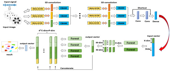
Figure 8.
The model structure of ADSD-gcForest.

Table 1.
Detailed parameters of the optimized network.
4. Experiments
4.1. Introduction of Datasets
The datasets used in the experiment were the Case Western Reserve University bearing dataset and the Canadian University of Ottawa bearing dataset. Two different bearings are contained in the Western Reserve University bearing dataset: drive end bearing SKF6205 and fan end bearing SKF6203. The drive end bearing included the two different sampling frequencies of 12 KHZ and 48 KHZ, while the sampling frequency of the fan end bearing was only 12 KHZ. Ten types of states are contained in each bearing dataset, which are normal state, inner ring failure, outer ring failure, and rolling element failure. Each fault state contains three different fault levels, represented by a fault diameter. A total of four different load conditions were applied when measuring the bearing data. A total of 8 normal samples, 53 outer ring damage samples, 23 inner ring damage samples and 11 rolling element damage samples were obtained. The Canadian Ottawa dataset is the bearing vibration signal of different health conditions measured under time-varying speed conditions, which had 36 datasets. The bearing conditions include: normal, inner ring failure and outer ring failure. The working speed conditions are speed increase, speed deceleration, deceleration after speed increase and speed increase after deceleration. Each dataset contains two channels, and channel 1 represents the vibration data measured by the accelerometer, channel 2 signifies the speed data measured by the encoder, the sampling frequency is 200 KHZ and the sampling duration is 10 s.
The drive end and the fan end bearing data of Western Reserve University used in this paper are at the sampling frequency of 12 KHZ, and for part of the dataset in Channel 1 of the University of Ottawa in Canada, the sample data used were randomly selected from the dataset, where B, IR and OR indicate that the fault location is located in the rolling element, inner ring and outer ring of the bearing, respectively. Moreover, 007, 014 and 021, respectively, indicate that the fault diameter is 0.1778 mm, 0.3556 mm and 0.5334 mm, and the number at the end indicates the size of the load. For example, “−1” means that the load is 1 horsepower. A total of 1000 samples were sampled for each fault category, and the sample ratio of training set to test set was 7:3. The details are shown in Table 2.
Table 2.
Sample distribution table.
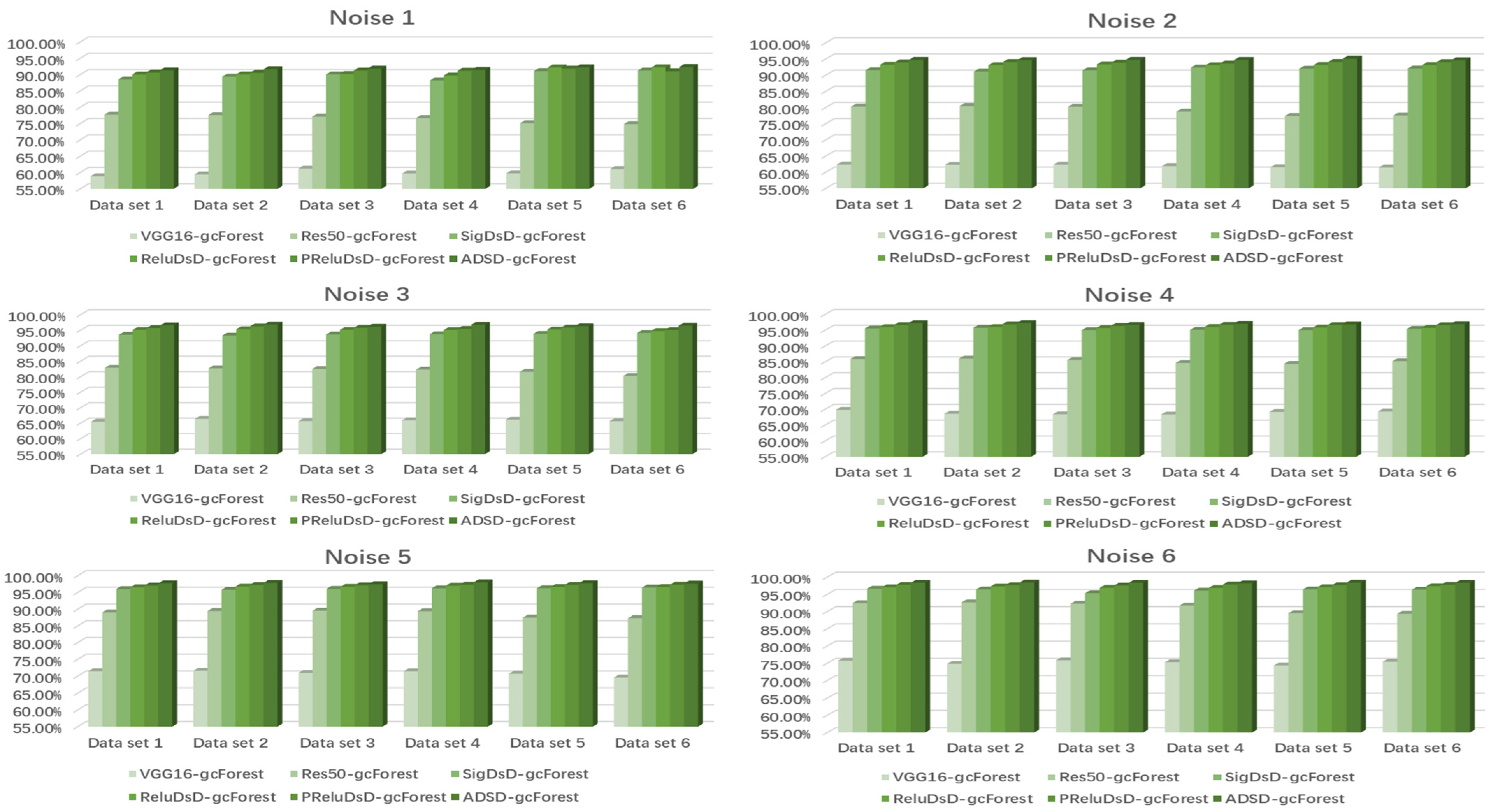
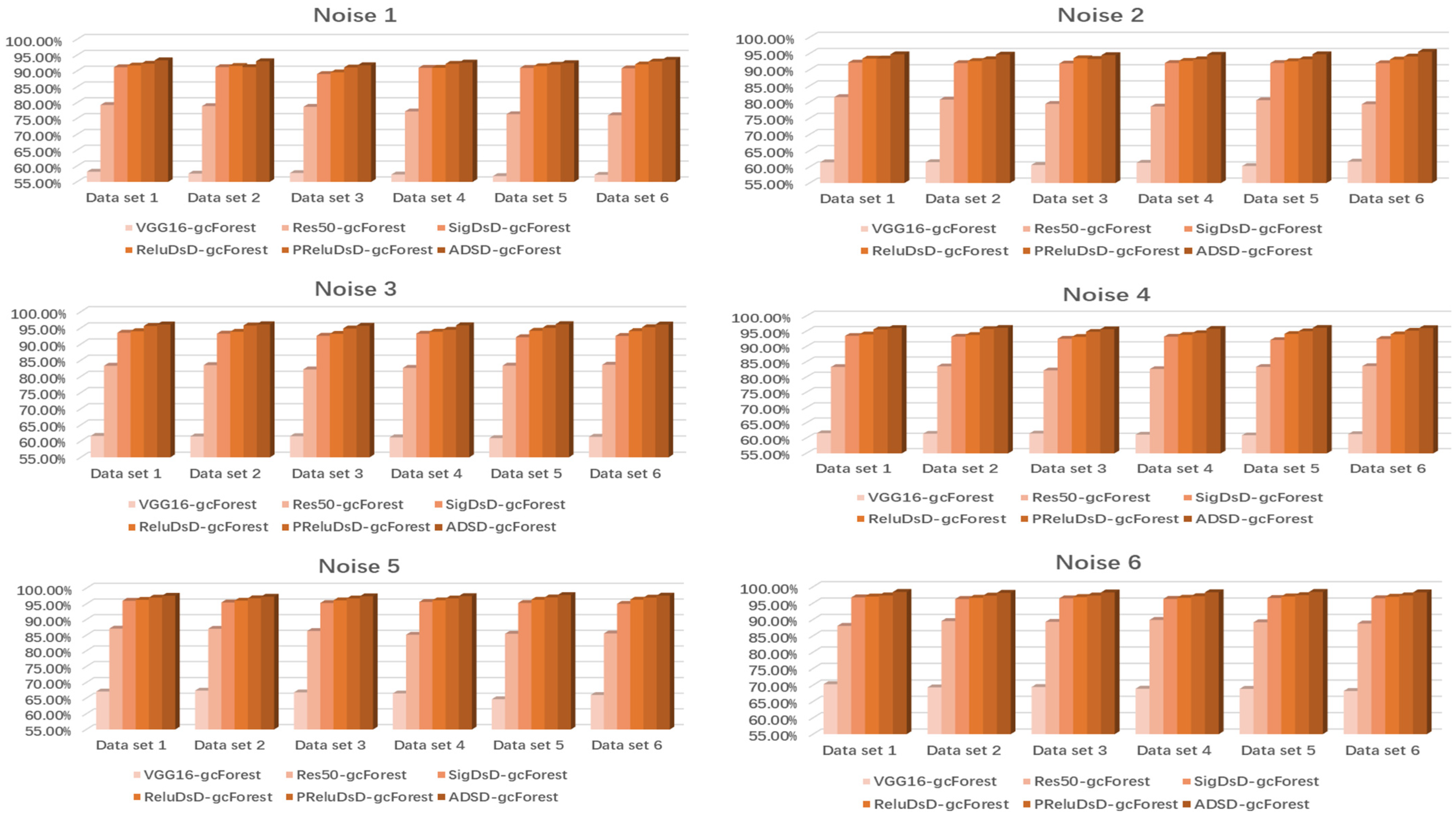
Six noises of different intensities were added to the sample dataset, namely, Noise 1, Noise 2, Noise 3, Noise 4, Noise 5 and Noise 6. Each type of noise contains three different types of noise. The proportions of the three noises in the six noises were Gaussian noise with signal-to-noise ratios of −4, −2, 0, 2, 4 and 6, salt and pepper noise, with ratios of 0.3, 0.25, 0.2, 0.15, 0.1 and 0.05, and Cauchy noise with position parameter 0 and scale parameter 1. gcForest was set as the classifier in all comparison methods, and SigDSD-gcforest means that the Sigmoid function is the activation function of the convolutional layers. Similarly, the activation functions of the convolutional layers in ReluDSD-gcforest and PReluDSD-gcforest are Relu and PRelu, respectively. The parameter settings of the ADSD-gcForest model were as follows: the network training parameters were set at a learning rate of 0.00005, the number of batch processing was 580, the number of iterations was 350, Adam was used as the optimization algorithm, the sliding window dimension used in MGS was 240, the number of trees in the random forests of MGS was 35 and the number of trees in a single random forest in the cascade forest was 150. The diagnostic effect is analyzed by comparing the accuracy rate, F1 value and Area Under Curve (AUC) value of different diagnostic models after training. The accuracy rate is generally expressed as , and FI value is calculated as , where TP refers to True Positives, FP represents True Negatives, FN indicates False Negatives and FP signifies False Positives. AUC is defined as the area under the area under curve. Generally, the higher the AUC value, the better the classification effect of the model.
4.2. Case Study 1: Performance of Drive End Bearing Fault Diagnosis
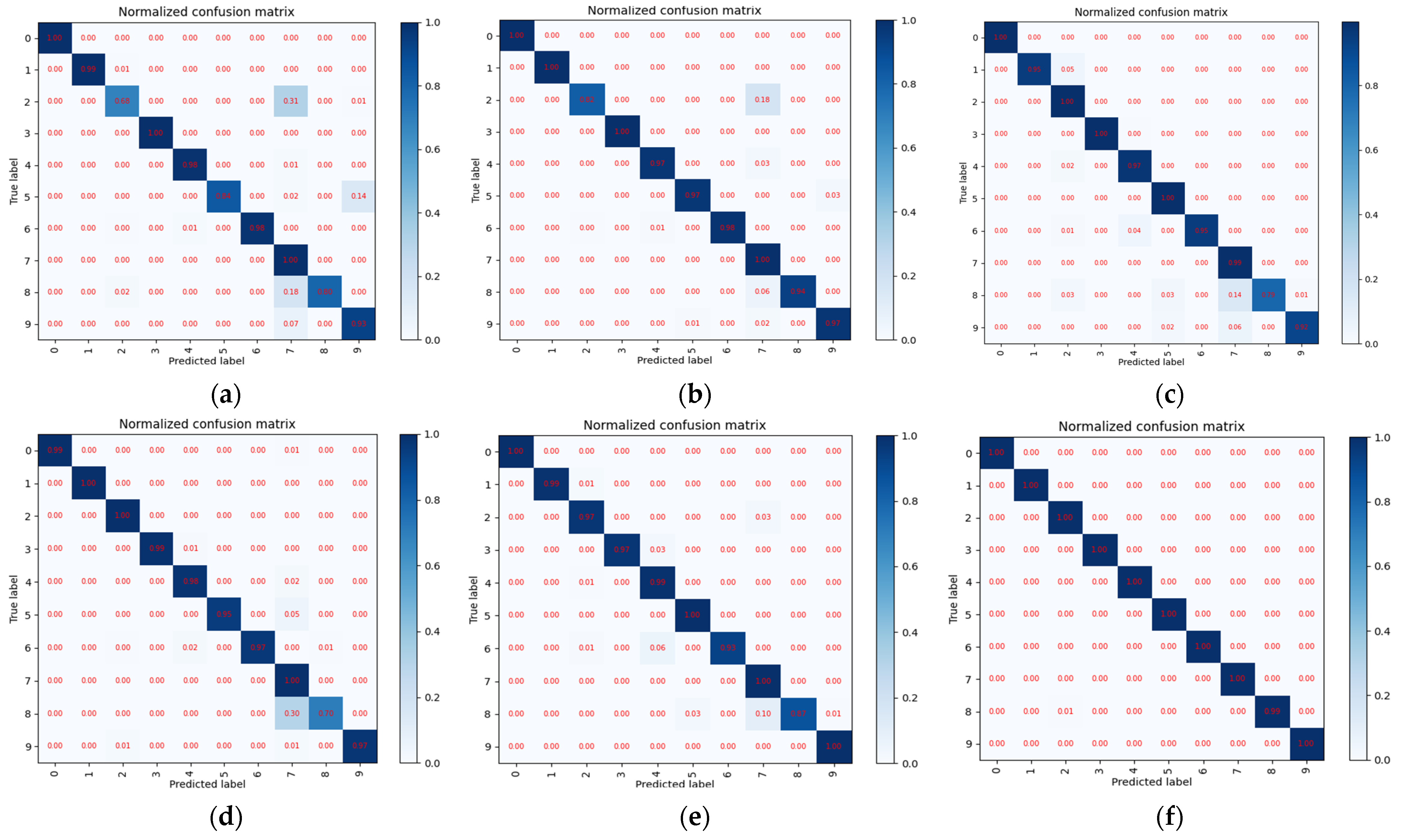
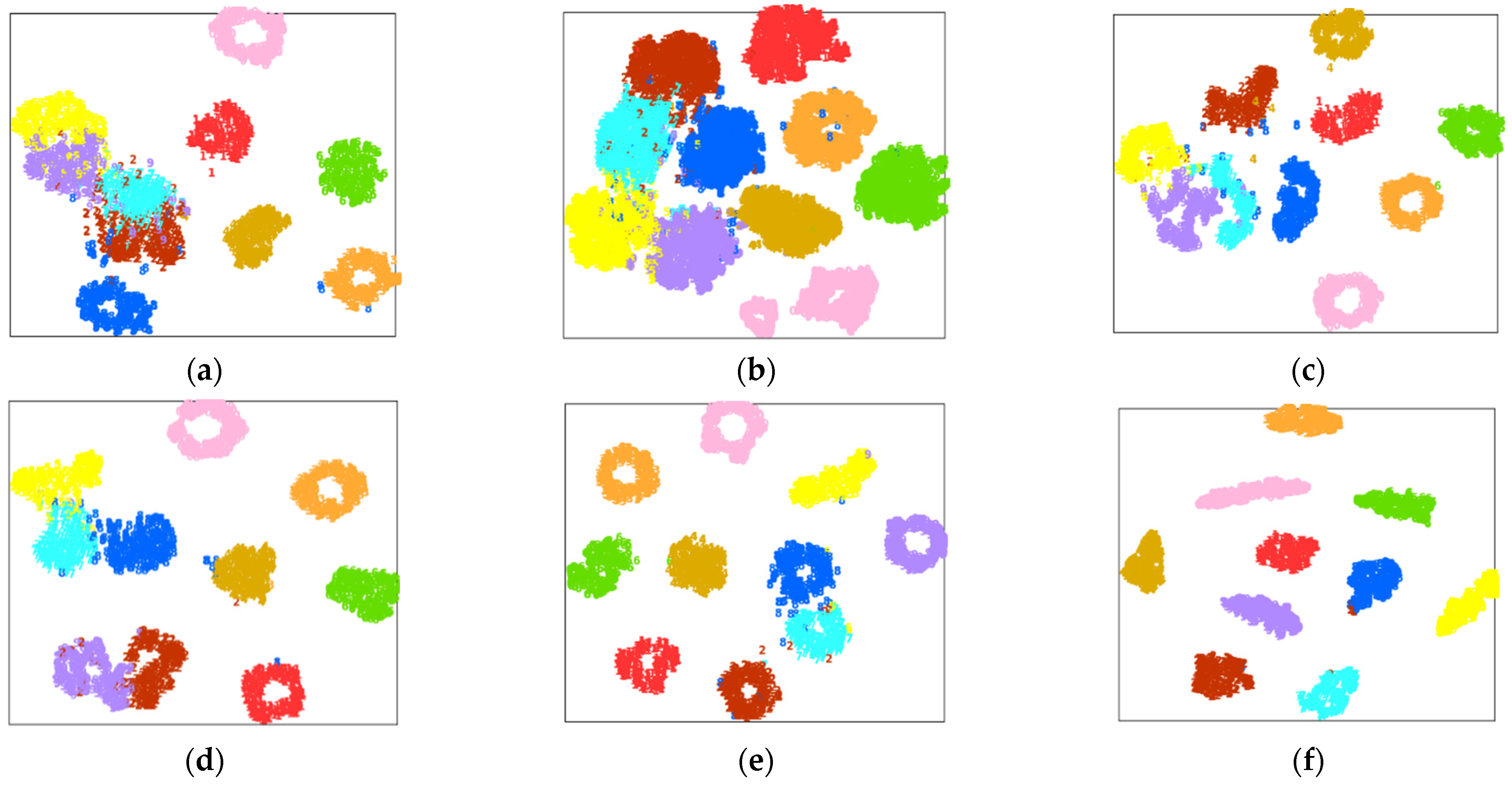
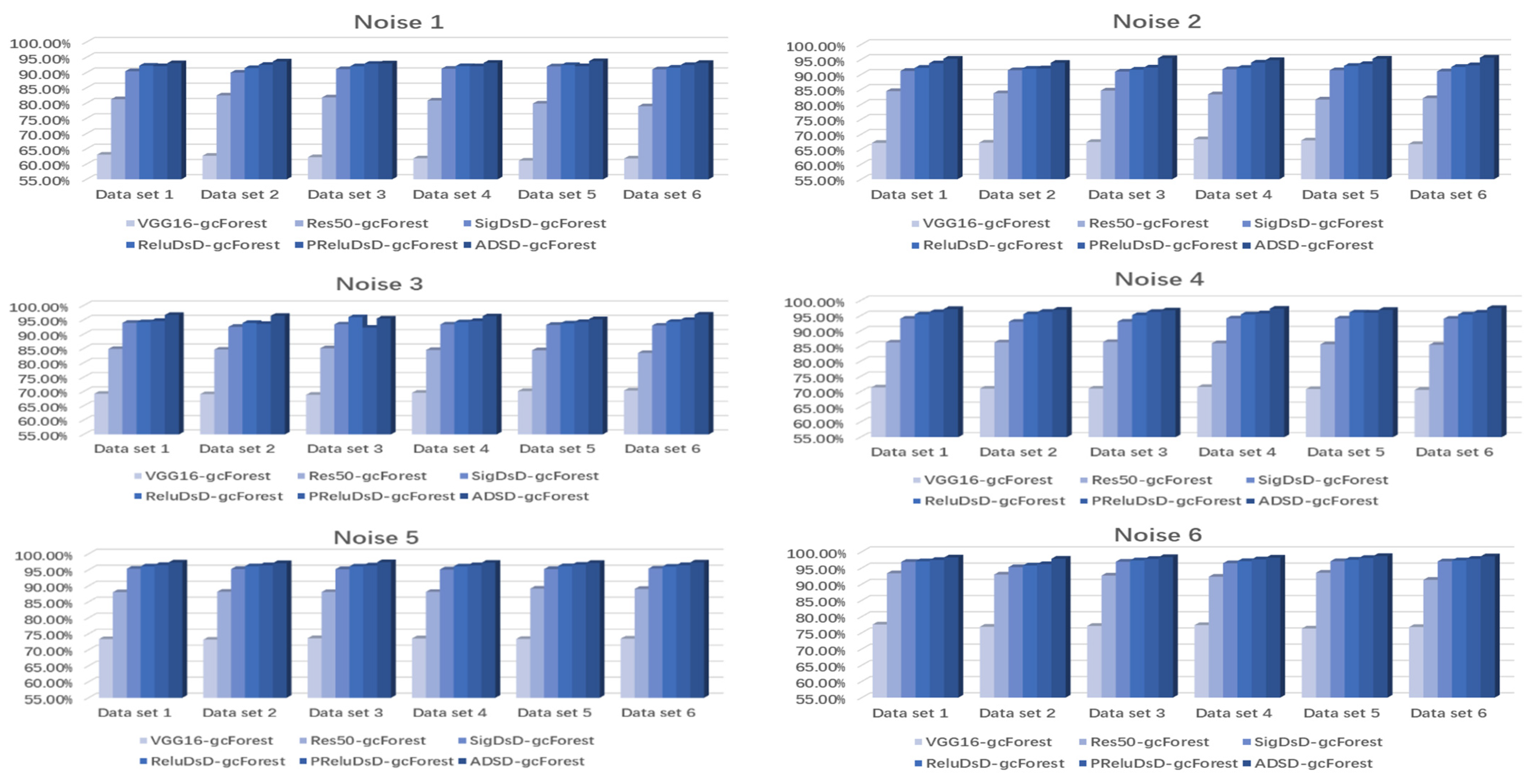
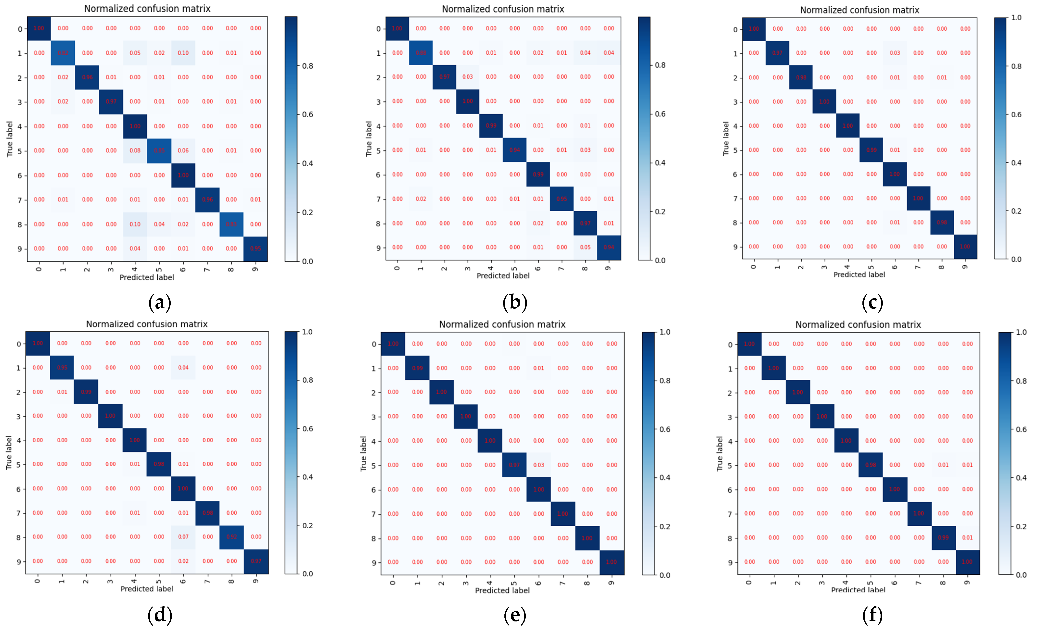
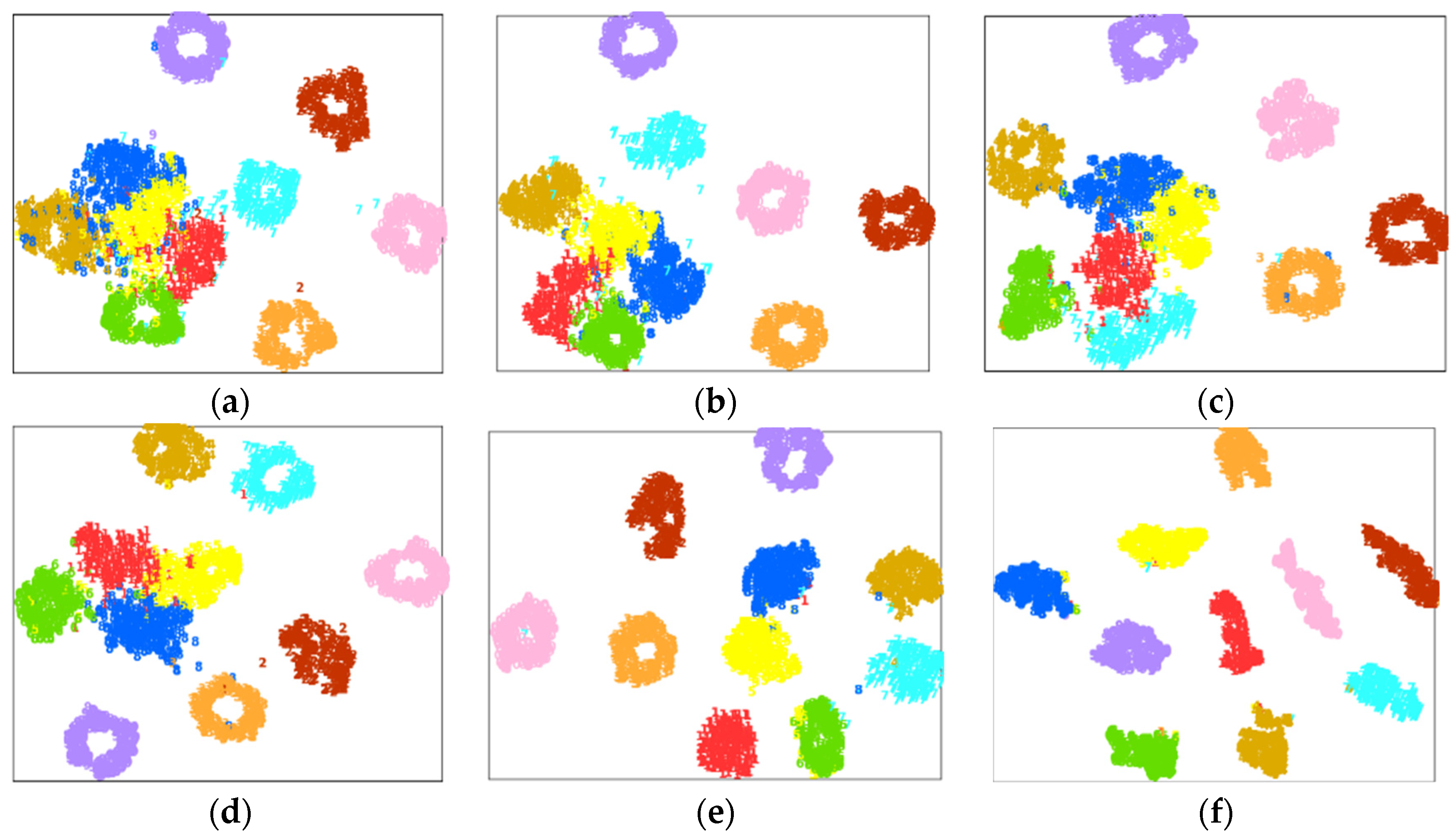
It can be seen from Figure 9 and Figure 10 that when the noise environment is Noise 1, after the sample is trained by the ADSD-gcForest model, there are three categories of samples with low recognition rates, and there is also a small amount of aliasing in the T-SNE image. In other noise environments, there are only one or two fault categories with a low recognition rate. It can be seen from Table 3 that, compared to other methods, the ADSD-gcForest model achieves the highest fault accuracy rate and F1 value under various noises and different working conditions. Among them, the VGG16-gcForest model obtained the lowest accuracy and the F1 values, which is about 26–35% lower than those of the ADSD-gcForest model, while the accuracy and F1 values of the Res50-gcForest model are about 18% higher than the VGG16-gcForest model. Since the Relu function can better solve the network convergence problem than the Sigmoid function, the accuracy and F1 values of the Relu-gcForest model are about 0.6–0.7% higher than that of the SigDSD-gcForest model, and PRelu updates the weight according to the input data, which makes the network have a certain adaptive optimization capability. The accuracy and F1 values obtained after training is about 1.3% higher than that of the Relu-gcForest model, but its values are still lower than the ADSD-gcForest model. Figure 11 mainly describes the comparison of the AUC values of different methods. From Figure 11, it can be found that the AUC values of ADSD-gcForest under different noises are the highest and all are above 92%, indicating that the ADSD-gcForest model has a good fault diagnosis effect. It can be seen from the experimental results presented above that the ADSD-gcForest model can more accurately diagnose drive-end bearing failures under different working conditions and strong noise interference with a high accuracy rate.
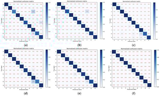
Figure 9.
Confusion matrix obtained by ADSD-gcforest model training (drive end). (a) Noise 1, (b) Noise 2, (c) Noise 3, (d) Noise 4, (e) Noise 5. (f) Noise 6.
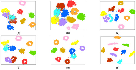
Figure 10.
T-SNE images obtained by ADSD-gcforest model training (drive end). (a) Noise 1, (b) Noise 2, (c) Noise 3, (d) Noise 4, (e) Noise 5. (f) Noise 6.
Table 3.
Comparison table of the accuracy (AC) and F1 values of driver end data.

Figure 11.
Comparison figures of the AUC of the driver end data under Noise 1, 2, 3, 4, 5 and 6.
4.3. Case Study 2: Performance of Fan End Bearing Fault Diagnosis
It can be seen from Figure 12 and Figure 13 that only when the noise environment is Noise 1, a few fault categories cannot be effectively identified. In other noise environments, the entire fault category can be accurately identified. It can be seen in Table 4 that the accuracy and F1 values obtained from the training of the VGG16-gcForest and Res50-gcForest models have dropped by approximately 1.5–1.6% compared to the driving end values. The overall accuracy and F1 value of the VGG16-gcForest model are between 61–75%. The accuracy and F1 values of the training of the SigDSD-gcForest, ReluDSD-gcForest and PreluDSD-gcForest models has also decreased. Among them, the most obvious decrease is SigDSD-gcForest, with a decrease from 0.3% to 0.4%, while the accuracy and F1 value of the PreluDSD-gcForest model drops by at least about 1.3–1.5%. The accuracy value and F1 values of the ADSD-gcForest model are the highest, and these values are similar to case study 1. Figure 14 depicts the AUC values obtained by different diagnostic methods under different noises. It can be found that the AUC values obtained by the ADSD-gcForest model are still the highest, which are close to those obtained in case study 1. Through the experimental results presented above, it can be found that the ADSD-gcForest model proposed in this paper can basically realize an effective fault diagnosis for different bearings under multiple working conditions.
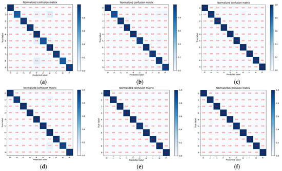
Figure 12.
Confusion matrix obtained by ADSD-gcForest model training (fan end). (a) Noise 1, (b) Noise 2, (c) Noise 3, (d) Noise 4, (e) Noise 5. (f) Noise 6.
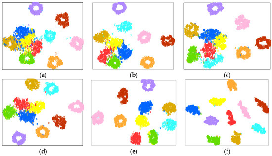
Figure 13.
T-SNE images obtained by ADSD-gcForest model training (fan end). (a) Noise 1, (b) Noise 2, (c) Noise 3, (d) Noise 4, (e) Noise 5. (f) Noise 6.
Table 4.
Comparison table of the accuracy (AC) and F1 values of the fan end data.
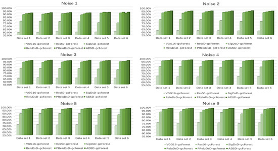
Figure 14.
Comparison figures of the AUC of the fan end data under Noise 1, 2, 3, 4, 5 and 6.
4.4. Case Study 3: Performance of the Ottawa Bearing Dataset
In order to further test the generalization and robustness of the ADSD-gcForest model, case study 3 focused on the University of Ottawa dataset, which was specifically divided into six datasets. The setting method of adding noise was the same as case study 1. The specific sample types are shown in Table 5. There were three operation conditions of the bearings in the datasets, i.e., normal (H), inner race fault (I) and out race fault (O), and also contained four speed transformation conditions, i.e., speed up (A), slow down (B), speed up and slow down (C) and slow down and speed up (D). The noise setting used in case study 3 is the same as the case study 1. The training parameter settings of the ADSD-gcForest model are as follows: the network training parameters were set to a learning rate of 0.00005, the number of batch processing was 550, the number of iterations was 350, Adam was used as the optimization algorithm, the sliding window dimension used in MGS was 240, the number of trees in the MGS random forest was 35 and the number of trees in a single random forest in the cascade forest was 150.
Table 5.
Sample distribution table.
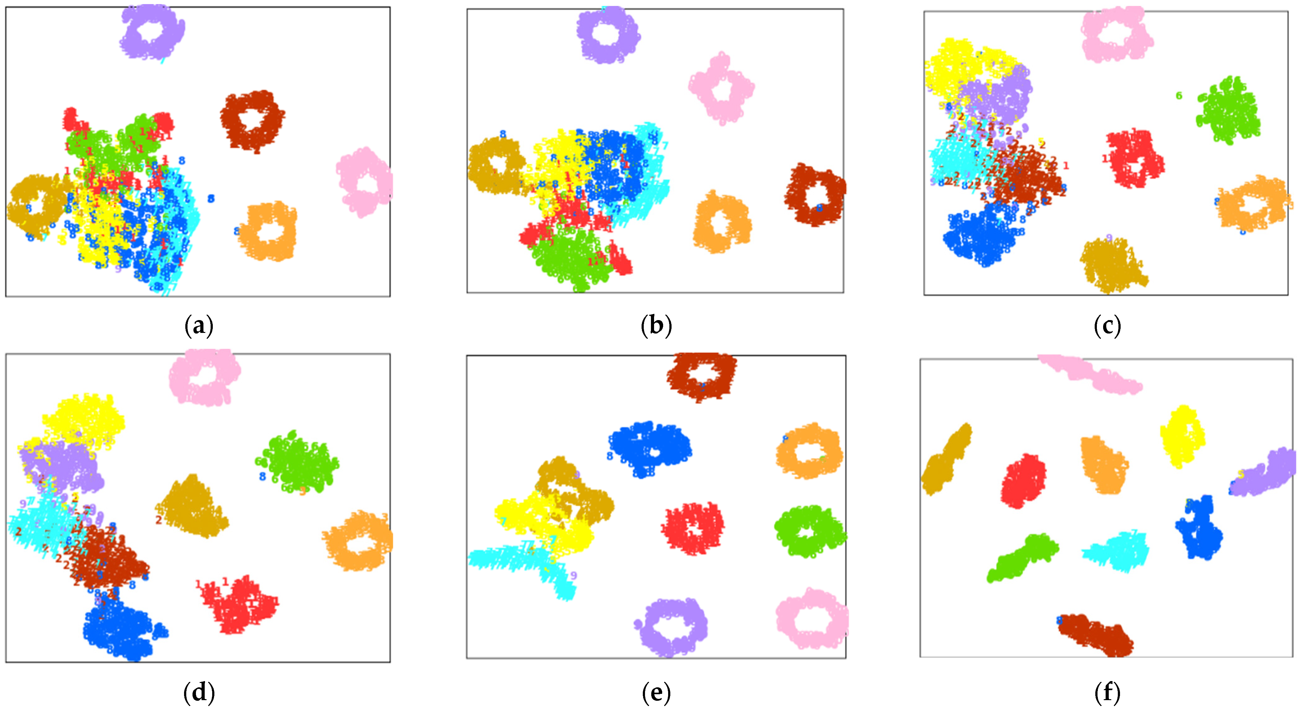
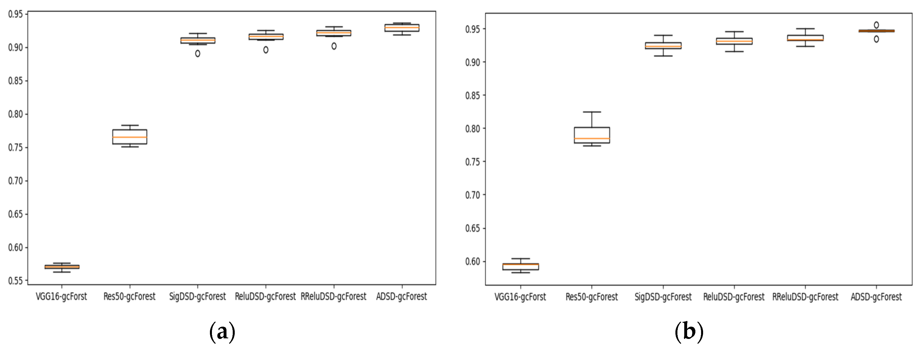
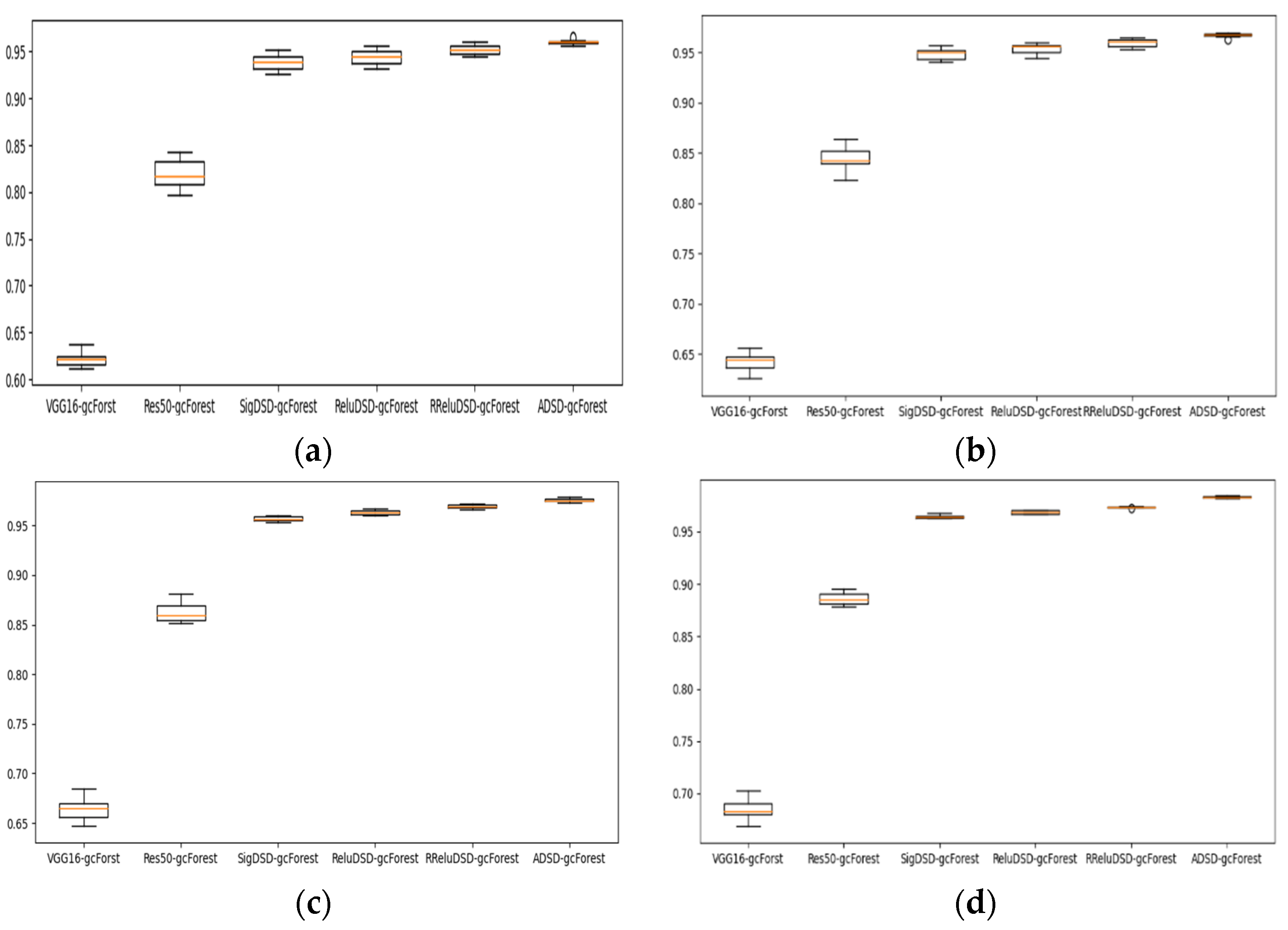
It can be seen from Figure 15 that, compared to case study 1 and case study 2, when the noise environment is Noise 1 and Noise 2, the degree of discrimination of some fault categories is lower, but in other noise environments, the fault categories can be accurately classified. It can be seen from Figure 16 and Figure 17 that the training accuracy of the ADSD-gcForest model is the highest and the value is relatively stable, while the fluctuation is small, which is consistent with the values in Table 6. At the same time, it can be found from Table 6 that the accuracy and F1 values obtained by training the VGG16-gcForest and Res50-gcForest models are significantly lower than case study 1 and case study 2. In Figure 16 and Figure 17, the accuracy of the two models also fluctuates significantly, and the accuracy of the other three models is more accurate. The rate values have also decreased, but the value fluctuations are relatively small. Figure 18 reflects the AUC values of different diagnostic models, from which it can be found that the AUC values of the ADSD-gcForest model are basically similar to the first two cases, but other diagnostic models have decreased. Through comparative experiments of three groups of different bearings, it can be seen that under different noise conditions and for bearing data under different working conditions, in one way, the ADSD-gcForest model can achieve effective fault feature extraction, while in another way, the use of the Meta-ACON activation function can easily and efficiently complete the self-adaptive optimization of the model structure and realize more accurate fault diagnosis.
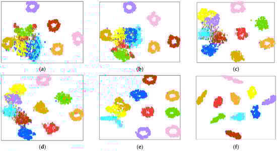
Figure 15.
T-SNE images obtained by ADSD-gcforest model training (Ottawa Bearing). (a) Noise 1, (b) Noise 2, (c) Noise 3, (d) Noise 4, (e) Noise 5. (f) Noise 6.
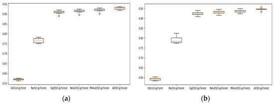
Figure 16.
Box plots of accuracy values under different noise conditions. (a) Noise 1, (b) Noise 2.
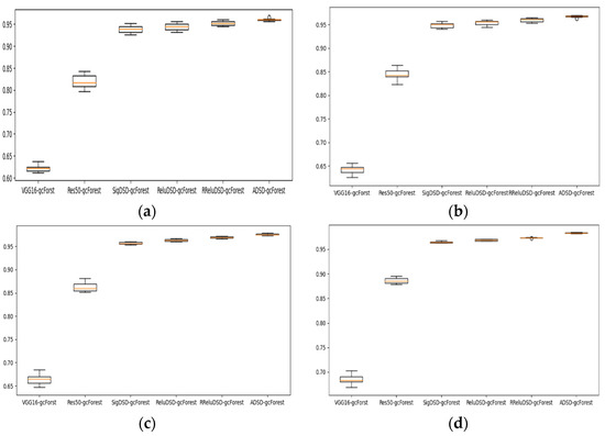
Figure 17.
Box plots of accuracy values under different noise conditions. (a) Noise 3, (b) Noise 4, (c) Noise 5, (d) Noise 6.
Table 6.
Comparison table of the accuracy (AC) and F1 values of the Ottawa dataset.
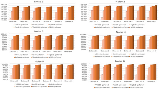
Figure 18.
Comparison figures of the AUC of the Ottawa dataset under Noise 1, 2, 3, 4, 5 and 6.
5. Conclusions
This paper proposes an adaptive ADSD-gcForest model. The model uses the VGG network as the basic framework. Multi-scale features of input samples can be extracted through deep separable dilated convolution, and then the CBAM to focus the core features is combined at different scales, the Meta-ACON activation function is integrated into all convolution layers in the network, so that the model can be optimized adaptively according to different input data, and the gcForest as the final classifier can provide the final result. In the experimental part of this paper, datasets of Western Reserve University and University of Ottawa are used, including three bearing data, and it can be seen that faults of different types of bearings under strong noise and multiple load conditions can be effectively diagnosed by the ADSD-gcForest model. This shows that the model proposed in this paper has good robustness. It can also be found that the method proposed in this paper has better improved the migration ability of the model, simplified the design process of the diagnostic model and effectively avoided the problem of repeatedly modifying the model structure.
In modern industrial production, multiple bearings are often required to work together; thus, the effective fault diagnosis of multiple bearings is a hot research topic. The ADSD-gcForest model proposed in this paper can simply optimize the model structure according to different bearing data with the help of the Meta-ACON activation function. It has a certain industrial application value, but the addition of the Meta-ACON activation function also increases the number of parameters of the model, which leads to a longer training time. Therefore, how to reduce the training parameters of the Meta-ACON activation function under the premise of ensuring high accuracy will become the focus of future research.
Author Contributions
Conceptualization: S.Z.; Methodology: S.Z. and Z.W.; Formal analysis and investigation: S.Z.; Writing—original draft preparation: S.Z.; Writing—review and editing: D.G. and S.Z. All authors have read and agreed to the published version of the manuscript.
Funding
This research received no external funding.
Institutional Review Board Statement
Not applicable.
Informed Consent Statement
Not applicable.
Data Availability Statement
The used data of bearing fault can be found in CWRU Data Center and University of Ottawa datasets are available online: https://csegroups.case.edu/bearingdatacenter/pages/welcome-case-western-reserve-university-bearing-data-center-website (accessed 18 Octorber 2021), https://data.mendeley.com/datasets/v43hmbwxpm/1 (accessed 20 Octorber 2021).
Conflicts of Interest
The authors declare no conflict of interest.
References
- Fan, J.; Qi, Y.; Liu, L.; Gao, X.; Li, Y. Application of an information fusion scheme for rolling element bearing fault diagnosis. Meas. Sci. Technol. 2021, 32, 075013. [Google Scholar] [CrossRef]
- Niu, G.; Wang, X.; Golda, M.; Mastro, S.; Zhang, B. An optimized adaptive PReLU-DBN for rolling element bearing fault diagnosis. Neurocomputing 2021, 445, 26–34. [Google Scholar] [CrossRef]
- Jie, D.; Zheng, G.; Zhang, Y.; Ding, X.; Wang, L. Spectral kurtosis based on evolutionary digital filter in the application of rolling element bearing fault diagnosis. Int. J. Hydromechatronics 2021, 4, 27–42. [Google Scholar] [CrossRef]
- Zhao, X.; Qin, Y.; Fu, H.; Jia, L.; Zhang, X. Blind source extraction based on EMD and temporal correlation for rolling element bearing fault diagnosis. Smart Resilient Transp. 2021, 3, 52–65. [Google Scholar] [CrossRef]
- Hou, W.; Ye, M.; Li, W. Rolling bearing fault classification based on improved stack noise reduction self-encoding. Chin. J. Mech. Eng. 2018, 54, 87–96. [Google Scholar] [CrossRef]
- Shao, H.; Jiang, H.; Zhang, X.; Niu, M. Rolling bearing fault diagnosis using an optimization deep belief network. Meas. Sci. Technol. 2015, 26, 115002. [Google Scholar] [CrossRef]
- Liang, T.; Wu, S.; Duan, W.; Zhang, R. Bearing fault diagnosis based on improved ensemble learning and deep belief network. J. Phys. Conf. Ser. 2018, 1074, 012154. [Google Scholar] [CrossRef]
- Ma, M.; Chen, X.; Wang, S.; Liu, Y.; Li, W. Bearing degradation assessment based on weibull distribution and deep belief network. In Proceedings of the IEEE International Symposium on Flexible Automation, Cleveland, OH, USA, 1–3 August 2016; pp. 382–385. [Google Scholar]
- Shao, S.; Sun, W.; Wang, P.; Gao, R.X.; Yan, R. Learning features from vibration signals for induction motor fault diagnosis. In Proceedings of the IEEE International Symposium on Flexible Automation, Cleveland, OH, USA, 1–3 August 2016; pp. 71–76. [Google Scholar]
- Han, T.; Yuan, J.H.; Tang, J.; An, L.Z. Intelligent composite fault diagnosis method of rolling bearing based on MWT and CNN. Mech. Transm. 2016, 40, 139–143. [Google Scholar]
- Liang, M.; Cao, P.; Tang, J. Tang. Rolling bearing fault diagnosis based on feature fusion with parallel convolutional neural network. Int. J. Adv. Manuf. Technol. 2020, 112, 819–831. [Google Scholar] [CrossRef]
- Pan, H.; He, X.; Tang, S.; Meng, F. An improved bearing fault diagnosis method using one-dimensional CNN and LSTM. J. Mech. Eng. 2018, 64, 443–452. [Google Scholar]
- Zhang, L.; Jing, L.; Xu, W.; Tan, J. Rolling bearing fault diagnosis based on convolutional noise reduction autoencoder and CNN. Modul. Mach. Tool Autom. Manuf. Technol. 2019, 6, 58–62. [Google Scholar]
- Yu, L.; Qu, J.; Gao, F.; Tian, Y. A novel hierarchical algorithm for bearing fault diagnosis based on stacked LSTM. Shock. Vib. 2019, 2019, 2756284. [Google Scholar] [CrossRef] [PubMed]
- Zhao, R.; Yan, R.; Wang, J.; Mao, K. Learing to monitor machine health with convolutional bi-directional lstm networks. Sensors 2017, 17, 273. [Google Scholar] [CrossRef] [PubMed]
- Yan, X.; Xu, Y.; Jia, M. Intelligent Fault Diagnosis of Rolling-Element Bearings Using a Self-Adaptive Hierarchical Multiscale Fuzzy Entropy. Entropy 2021, 23, 1128. [Google Scholar] [CrossRef] [PubMed]
- Yong, Z.; Zhang, X.; Da, N. Research on 3D Object Detection Method Based on Convolutional Attention Mechanism. J. Phys. Conf. Ser. 2021, 1848, 012097. [Google Scholar] [CrossRef]
- Cao, Q.; Yu, L.; Wang, Z.; Zhan, S.; Quan, H.; Yu, Y.; Khan, Z.; Koubaa, A. Wild Animal Information Collection Based on Depthwise Separable Convolution in Software Defined IoT Networks. Electronics 2021, 10, 2091. [Google Scholar] [CrossRef]
- Ma, N.; Zhang, X.; Liu, M.; Sun, J. Activate or Not: Learning Customized Activation. In Proceedings of the IEEE/CVF Conference on Computer Vision and Pattern Recognition, Seattle, WA, USA, 13–19 June 2020. [Google Scholar]
- Zhang, N.; Cui, F.; Jiang, B.; He, X. Rotating machinery gearbox fault diagnosis method integrating SDP and CNN. Ind. Control. Comput. 2021, 34, 89–91. [Google Scholar]
- Zhao, L.; Xu, L.; Liu, Y.; Liu, J.; Huang, X. Transformer mechanical fault diagnosis method based on point symmetry transformation and image matching. Trans. Chin. Soc. Electr. Eng. 2021, 36, 3614–3626. [Google Scholar]
- Yin, Q.; Yang, W.; Ran, M.; Wang, S. FD-SSD: An improved SSD object detection algorithm based on feature fusion and dilated convolution. Signal Processing Image Commun. 2021, 98, 116402. [Google Scholar] [CrossRef]
- Yuhui, Z.; Mengyao, C.; Yuefen, C.; Zhaoqian, L.; Yao, L.; Kedi, L. An Automatic Recognition Method of Fruits and Vegetables Based on Depthwise Separable Convolution Neural Network. J. Phys. Conf. Ser. 2021, 1871, 012075. [Google Scholar] [CrossRef]
- Teng, Y.; Gao, P. Generative Robotic Grasping Using Depthwise Separable Convolution. Comput. Electr. Eng. 2021, 94, 107318. [Google Scholar] [CrossRef]
- Liu, T.; Pang, B.; Zhang, L.; Yang, W.; Sun, X. Sea Surface Object Detection Algorithm Based on YOLO v4 Fused with Reverse Depthwise Separable Convolution (RDSC) for USV. J. Mar. Sci. Eng. 2021, 9, 753. [Google Scholar] [CrossRef]
- Chen, Y.; Zhang, X.; Chen, W.; Li, Y.; Wang, J. Research on Recognition of Fly Species Based on Improved RetinaNet and CBAM. IEEE Access 2020, 8, 102907–102919. [Google Scholar] [CrossRef]
- Canayaz, M. C+EffxNet: A novel hybrid approach for COVID-19 diagnosis on CT images based on CBAM and EfficientNet. Chaos Solitons Fractals 2021, 151, 111310. [Google Scholar] [CrossRef] [PubMed]
- Niu, C.; Nan, F.; Wang, X. A super resolution frontal face generation model based on 3DDFA and CBAM. Displays 2021, 69, 102043. [Google Scholar] [CrossRef]
- Sun, Z.; Li, M.; Zhang, J.; Hu, B.; Qi, G.; Zhu, Y. Transient Voltage Stability Assessment Method based on gcForest. J. Phys. Conf. Ser. 2021, 1914, 012025. [Google Scholar] [CrossRef]
- Liu, H.; Zhang, N.; Jin, S.; Xu, D.; Gao, W. Small sample color fundus image quality assessment based on gcforest. Multimed. Tools Appl. 2020, 80, 17441–17459. [Google Scholar] [CrossRef]
Publisher’s Note: MDPI stays neutral with regard to jurisdictional claims in published maps and institutional affiliations. |
© 2022 by the authors. Licensee MDPI, Basel, Switzerland. This article is an open access article distributed under the terms and conditions of the Creative Commons Attribution (CC BY) license (https://creativecommons.org/licenses/by/4.0/).