The Mack Chain Ladder and Data Granularity for Preserved Development Periods

Abstract

This paper is concerned with the choice of data granularity for the application of the Mack chain ladder model to forecast a loss reserve. It is a sequel to a related paper by Taylor, which considers the same question for the EDF chain ladder model. As in the earlier paper, it considers the question as to whether a decrease in the time unit leads to an increase or decrease in the variance of the loss reserve estimate. The question of whether a Mack chain ladder that is valid for one time unit (here called mesh size) remains so for another is investigated. The conditions under which the model does remain valid are established. There are various ways in which the mesh size of a data triangle may be varied, two of them of particular interest. The paper examines one of these, namely that in which development periods are preserved. Two versions of this are investigated: 1. the aggregation of development periods without change to accident periods; 2. the aggregation of accident periods without change to development periods. Taylor found that, in the case of the Poisson chain ladder, an increase in mesh size always increases the variance of the loss reserve estimate (subject to mild technical conditions). The case of the Mack chain ladder is more nuanced in that an increase in variance is not always guaranteed. Whether or not an increase or decrease occurs depends on the numerical values of certain of the age-to-age factors actually observed. The threshold values of the age-to-age factors at which an increase transitions to a decrease in variance are calculated. In the case of a change in the mesh of development periods, but with no change to accident periods, these values are computed for one particular data set, where it is found that variance always increases. It is conjectured that data sets in which this does not happen would be relatively rare. The situation is somewhat different when changes in mesh size over accident periods are considered. Here, the question of an increase or decrease in variance is more complex, and, in general terms, the occurrence of an increase in variance with increased mesh size is less likely.

1. Introduction

1.1. Background

The chain ladder is a widely used model for insurance loss reserving (Mack 1993; Taylor 1985, 2000; Wüthrich and Merz 2008). The data set to which it is applied is typically triangular, with rows labelled by accident period and columns by development period.

Accident and development periods are commonly years, but other units of time are possible, e.g., quarters, months, and weeks. As the time unit is decreased, the number of data points increases, but the volatility of each point increases. This leads to a question as to whether a decrease in the time unit leads to an increase or decrease in the variance of the loss reserve estimate. A natural companion to this question is whether there is an optimal time unit at which the variance of the forecast loss reserve is minimized.

A parallel question on the effects of mesh size on modelling and forecasting arises in a wide range of scientific areas. Taylor (2025) cites references.

The prior actuarial literature contains little comment on these matters, but Taylor (2025) investigated the question in relation to the EDF chain ladder (Wüthrich and Merz 2008; Taylor 2009), where EDF refers to the exponential dispersion family, and particularly the Poisson chain ladder. The conclusion in this last case was subject to a number of conditions, but, in broad terms, it was that a choice of the most granular data possible (i.e., a choice of accident and development periods of short duration) would minimize the variance of the forecast loss reserve.

1.2. Purpose of the Paper

Taylor (2025) noted that there were two distinct formulations of the chain ladder model, namely the EDF chain ladder referred to above and the Mack chain ladder (Mack 1993). Whereas Taylor investigated the former, the present paper considers similar questions of data granularity in relation to the Mack chain ladder.

The present paper thus discusses the influence of data granularity on the variance of the loss reserve forecast by the Mack chain ladder. Under suitable conditions, it is possible to identify the granularity that minimizes this variance.

In Taylor (2025), a distribution from the EDF was assigned to each observation. This enabled an appeal to sufficient statistics in the search for minimum variance unbiased estimators (“MVUEs”), and these statistics carried much of the theoretical load in that paper. By contrast, the Mack model is distribution-free, so sufficient statistics cannot be defined. The identification of MVUEs must proceed by different means.

1.3. Layout of the Paper

The paper considers changes in mesh size on the triangular data set, which is to say changes in the units of time used for accident and development periods. The effect of an increase in mesh size (i.e., an increase in the amount of time spanned by one of these periods) on the variance of the estimated loss reserve is investigated.

There are various ways in which the mesh size of a data set can be varied. Some are more sensible than others, and two fundamental types of variation were identified in Taylor (2025), specifically those that preserve

• Calendar periods;
• Development periods.

These types of variation are described in Section 2, where a specific notation is developed for each type of variation to allow translation between the original data set and that resulting from the change in mesh size.

Both types of variation are deserving of study in the context of the Mack chain ladder. However, considerations of space have limited the present paper to just one, namely changes in mesh size that preserve development periods. Those that preserve calendar periods may be explored in a separate paper.

Section 3 reviews the Mack chain ladder model, including its forecast of loss reserve, with an emphasis on the variance of the quantity under forecast.

Section 4 examines the effect of changed mesh size on the variance of the loss reserve when the change preserves development periods. First, the conditions are established under which the Mack chain ladder continues to be a valid model under changes in mesh (Section 4.1). In the cases where the Mack chain ladder remains a valid model, the effect of the changed mesh on the variance of the estimated loss reserve is then calculated.

Two cases are considered:

• That in which the development period mesh is changed (Section 4.2.1);
• That in which the accident period mesh is changed (Section 4.2.2).

2. Notation and Mathematical Preliminaries

The notational and mathematical apparatus required here is much the same as in Taylor (2025), and the majority of it is taken from that source.

2.1. Fundamentals

Let $i=\mathrm{1,2},\dots ,I$ denote the accident period and $j=\mathrm{1,2},\dots ,I$ the development period. Taylor (2025) denoted the range of $j$ as $\mathrm{0,1},\dots ,I-1$ but the present notation will be more natural later when development periods are merged and a notation is required for this.

Let $Y_{ij}$, with mean ${\mu }_{ij}$, denote the random variable representing the amount of claim payments during development period $j$ of accident period $i$. These quantities are usually referred to as incremental claim payments. For the moment, all accident and development periods are of equal duration, though this will change later.

A calendar period consists of all those combinations of $i$ and $j$ such that $i+j$ is constant. For definiteness, label the calendar $t$ if $i+j-1=t$.

It will be assumed that a standpoint is taken at the end of calendar period $I$ and one is in possession of certain data from calendar periods $\mathrm{1,2},\dots ,I$. Specifically, these data comprise the claim triangle ${\mathcal{D}}_U=\left\{Y_{ij}:i=1,\dots ,I,j=1,\dots ,I-i+1\right\}$. This will be referred to as the upper triangle. One wishes to use these data to forecast the lower triangle ${\mathcal{D}}_L=\left\{Y_{ij}:i=2,\dots ,I,j=I-i+2,\dots ,I\right\}.$ Let ${\mathcal{D}=\mathcal{D}}_U\cup {\mathcal{D}}_L$.

In a loss-reserving context, a realization of the upper triangle will have been observed. This will be denoted ${\mathcal{d}}_U$, which is the same as ${\mathcal{D}}_U$ with each random variable $Y_{ij}$ replaced by its realization $y_{ij}$.

It will also be convenient to define cumulative claim payments. Thus, define

$$C_{ij}= \sum _{k=1}^j{Y}_{ik} ,$$

(1)

which is the random variable representing the amount of cumulative claim payments up to the end of development period $j$ of accident period $i$. Further, let $c_{ij}$ be defined in the same way in terms of the $y_{ik}$ so that $c_{ij}$ is a realization of $C_{ij}$.

It is assumed that there is no claim activity beyond development period $I$, in which case $C_{iI}$ is the ultimate claim cost of accident period $i$.

The objective of the loss-reserving exercise is to forecast unobserved lower triangle. This will be denoted ${\widehat{\mathcal{D}}}_L$, which is the same as ${\mathcal{D}}_L$ with each random variable $Y_{ij}$ replaced by its forecast ${\widehat{Y}}_{ij}$.

The upper and lower triangles have been defined in terms of incremental claim payments. It will sometimes be convenient to define them in terms of cumulative claim payments, e.g., ${\mathcal{D}}_U=\left\{C_{ij}:i=1,\dots ,I,j=0,\dots ,I-i+1\right\}$. As there is an equivalence relation between the two forms of triangle, the terms upper and lower triangle will be used, with a slight abuse of terminology, to refer to either form, provided that the context removes any ambiguity.

Let ${\mathcal{R}}_i$ denote row $i$ of the incremental ${\mathcal{d}}_U$, i.e., ${\mathcal{R}}_i=\left\{y_{ij}:j=1,\dots ,I-i+1\right\}$, and let $r_j$ denote the sum of this row:

$$r_j=\sum _{{\mathcal{R}}_i}{y}_{ij}= c_{i,I-i+1} .$$

(2)

Further, let ${\mathcal{C}}_j$ denote column $j$ of the cumulative ${\mathcal{d}}_U$, i.e., ${\mathcal{C}}_j=\left\{c_{ij}:i=1,\dots ,I-j+1\right\}$, and let $s_j$ denote the sum of this column:

$$s_j=\sum _{{\mathcal{C}}_j}{c}_{ij}= \sum _{i=1}^{I-j+1}{c}_{ij} .$$

(3)

It will also be convenient to define

$$s_j^{-}= \sum _{i=1}^{I-j}{c}_{ij} .$$

(4)

As noted above, $C_{iI}$ is the ultimate claim cost of accident period $i$, and so ${\widehat{C}}_{iI}$ is an estimate of this quantity. The amount of outstanding losses (the loss reserve) for this accident period is equal to

$$L_i=C_{iI}-C_{i,I-\mathrm{i}+1},$$

(5)

and is estimated by

$${\widehat{L}}_i={\widehat{C}}_{iI}-c_{i,I-\mathrm{i}+1}.$$

(6)

The total reserve for all accident periods of interest is

$$L=\sum _{i=2}^I{L}_i,$$

(7)

which is estimated by

$$\widehat{L}=\sum _{i=2}^I{\widehat{L}}_i.$$

(8)

For a generic random variable $X$, the notation $X ~ \left(\mu ,{\sigma }^2\right)$ will mean that $X$ has mean and variance $\mu ,{\sigma }^2$ with no specified distribution.

2.2. Mesh Size

2.2.1. Preservation of Calendar Periods

Section 2.1 is phrased in terms of accident, developmentm and calendar periods, without any specification of the meaning of “period”. Often, in the literature, this unit is a year. But it need not be; it might be a quarter, month, week, or any other convenient length of time. This will be referred to as the mesh size of the data triangle.

Consider how the mesh size might be changed. Suppose that, in ${\mathcal{D}}_U$, $I=Nq$ for some strictly positive integers $N,q$. The mesh size can be changed from one unit of time to $q$ units. There will then be $N$ accident and development periods, instead of the original $I$.

An example would be the case in which the units of time in ${\mathcal{D}}_U$ are quarters and $I=40,N=10,q=4$. Here, the mesh size is changed from quarters to years, and ${\mathcal{D}}_U$ contains 10 accident and development years.

In the case of general $N$ and $q$, the change of mesh will induce a new upper triangle ${\mathcal{D}}_U^{\ast }$ in which row $i^{\ast }$ will be obtained from the merger of rows $q\left(i^{\ast }-1\right)+1,q\left(i^{\ast }-1\right)+2,\dots ,q{i}^{\ast }$ from ${\mathcal{D}}_U$.

Now suppose, in addition, that the change of mesh is required to preserve calendar periods. By this is meant that calendar period $t^{\ast }$ in ${\mathcal{D}}_U^{\ast }$ will comprise calendar periods $q\left(t^{\ast }-1\right)+1,q\left(t^{\ast }-1\right)+2,\dots ,q{t}^{\ast }$ from ${\mathcal{D}}_U$.

For given $i^{\ast }$ and $t^{\ast }$, development period $j^{\ast }=t^{\ast }-i^{\ast }+1$. Then the $\left(i^{\ast },j^{\ast }\right)$ cell of ${\mathcal{D}}_U^{\ast }$ will consist of all pairs of $\left(q\left(i^{\ast }-1\right)+r,\left[q\left(t^{\ast }-1\right)+s\right]-\left[q\left(i^{\ast }-1\right)+1+r\right]\right),r,s=1,\dots ,q$ from ${\mathcal{D}}_U$ such that the second member of the pair is non-negative. Equivalently, it consists of all pairs $\left(q\left(i^{\ast }-1\right)+r,max\left[0,q\left(j^{\ast }-1\right)+\left(s+1-r\right)\right]\right),r,s=1,\dots ,q$. Let $Y_{i^{\ast }{j}^{\ast }}^{\ast },C_{i^{\ast }{j}^{\ast }}^{\ast }$ be defined in the same way as $Y_{ij},C_{ij}$ but for the $\left(i^{\ast },j^{\ast }\right)$ cell of ${\mathcal{D}}_U^{\ast }$.

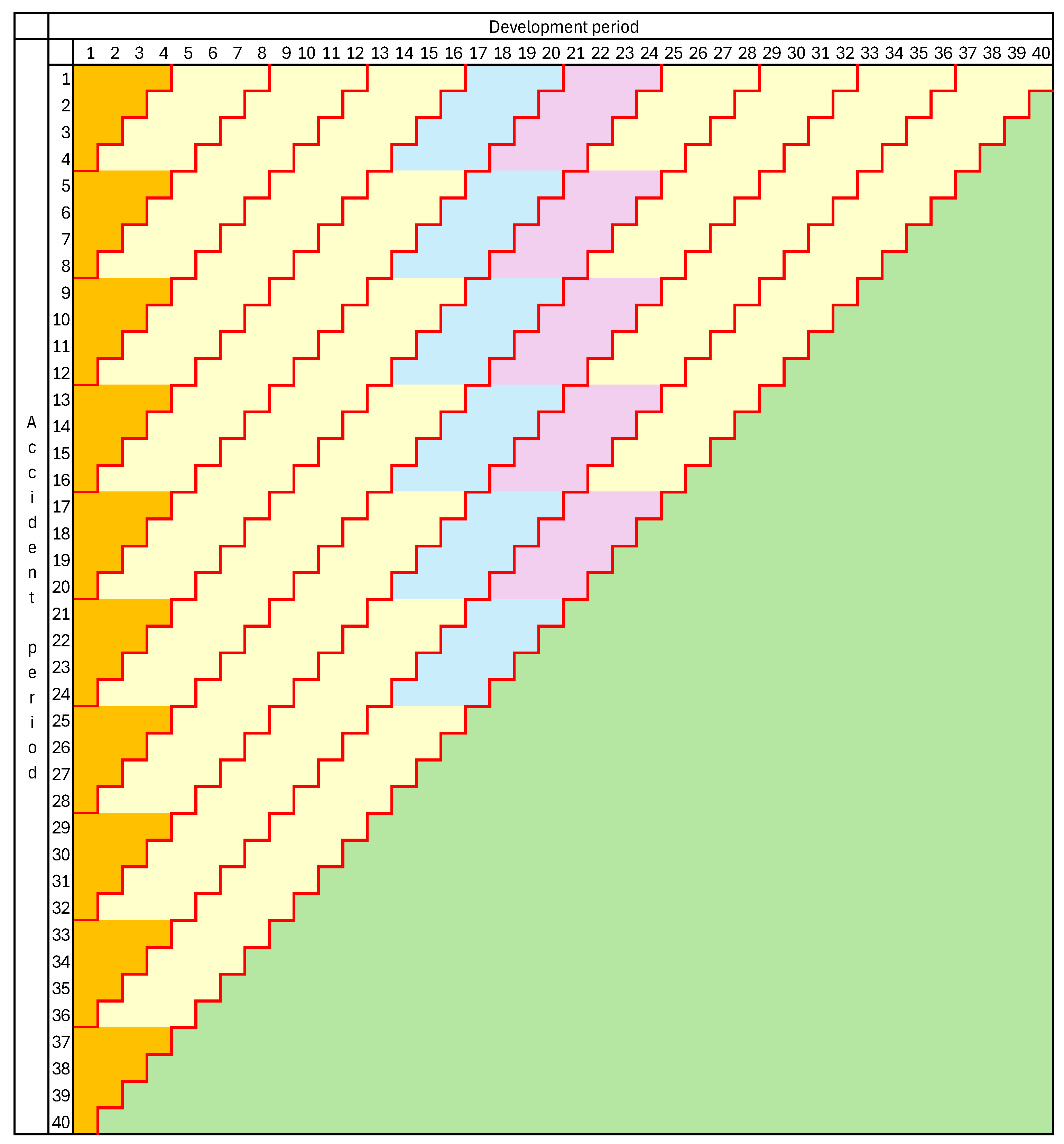
This is the form of aggregation from unit to $q$-unit periods commonly used in commercial practice. It is illustrated in Figure 1, in which a $40\times 40$ quarterly triangle is collapsed to a $10\times 10$ yearly triangle. The upper triangle is shaded yellow, and the lower one is shaded green. Calendar years are delineated by the red diagonals. Development years 5 and 6 are shaded blue and purple, respectively. Development year 1 is also shown in orange to illustrate its exceptional nature.

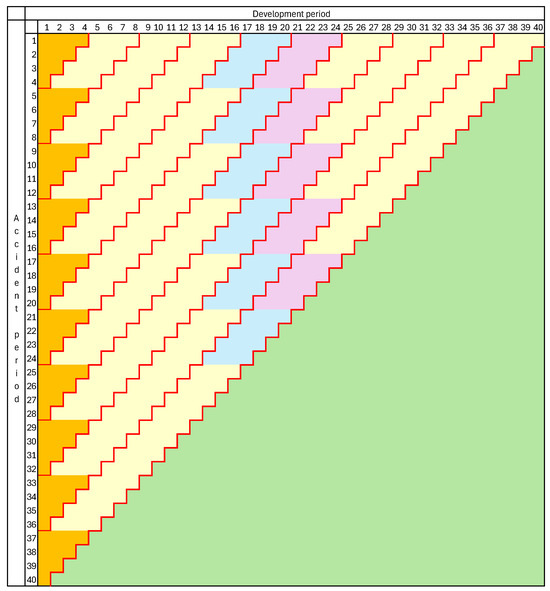
Figure 1. Change of mesh size from quarterly to yearly.

It will also be useful to define the following quantities in parallel with $s_j$ and $s_j^{-}$:

$$s_{j^{\ast }}^{\ast }= \sum _{i=1}^{N-j^{\ast }+1}{c}_{i^{\ast }{j}^{\ast }}^{\ast } ,$$

(9)

$$s_{j^{\ast }}^{\ast -}= \sum _{i=1}^{N-j^{\ast }}{c}_{i^{\ast }{j}^{\ast }}^{\ast } .$$

(10)

2.2.2. Preservation of Development Periods

It is seen in Figure 1 that the quarterly development periods that contribute to a specific yearly development period differ by accident quarter. Although this is standard commercial practice, one might regard this as sometimes undesirable.

An alternative is as follows. Define merged accident periods exactly as in Section 2.2.1, but define merged development periods in such a way that, for all accident periods, development period $j^{\ast }$ always consists of the same development periods from ${\mathcal{D}}_U$.

In this case, there is no requirement that accident and development periods be subject to the same mesh size. There is not even a requirement that all development periods be of the same duration.

To develop a notation for changed mesh size, we commence with the ordered set $\left\{0,\dots ,I\right\}$. This is the set labels for (unmerged) development periods, supplemented by a zero. The reason for this is that the development period label $j$ will be taken to relate to the end of that period, and so the zero denotes the point of commencement of development period 1. Then $\left\{0,\dots ,I\right\}$ will span the entire duration of the original $I$ development periods.

Now introduce $J^{\ast }+1$ integer cut-points ${\omega }_{j^{\ast }},j^{\ast }=0,\dots ,J^{\ast }$ to partition the set $\left\{0,\dots ,I\right\}$ with ${\omega }_0=0,{\omega }_{J^{\ast }}=I$. The segments of this partition are merged development periods. There are $J^{\ast }$ of these, and the $j^{\ast }$-th is the union of the unmerged development periods ${\omega }_{j^{\ast }-1}+1,\dots ,{\omega }_{j^{\ast }},j^{\ast }=1,\dots ,J^{\ast }$ and is of duration ${\omega }_{j^{\ast }}-{\omega }_{j^{\ast }-1}$ time periods.

A simple example would be similar to the one introduced in Section 2.2.1, in which the original development periods are quarterly, and the mesh size is changed from quarterly to annual. In this case, with $I=40$, one sets ${\omega }_{j^{\ast }}=4j^{\ast }$, and the merged (annual) development period $j^{\ast }$ comprises unmerged development periods $4\left(j^{\ast }-1\right)+r,r=\mathrm{1,2},\mathrm{3,4}$.

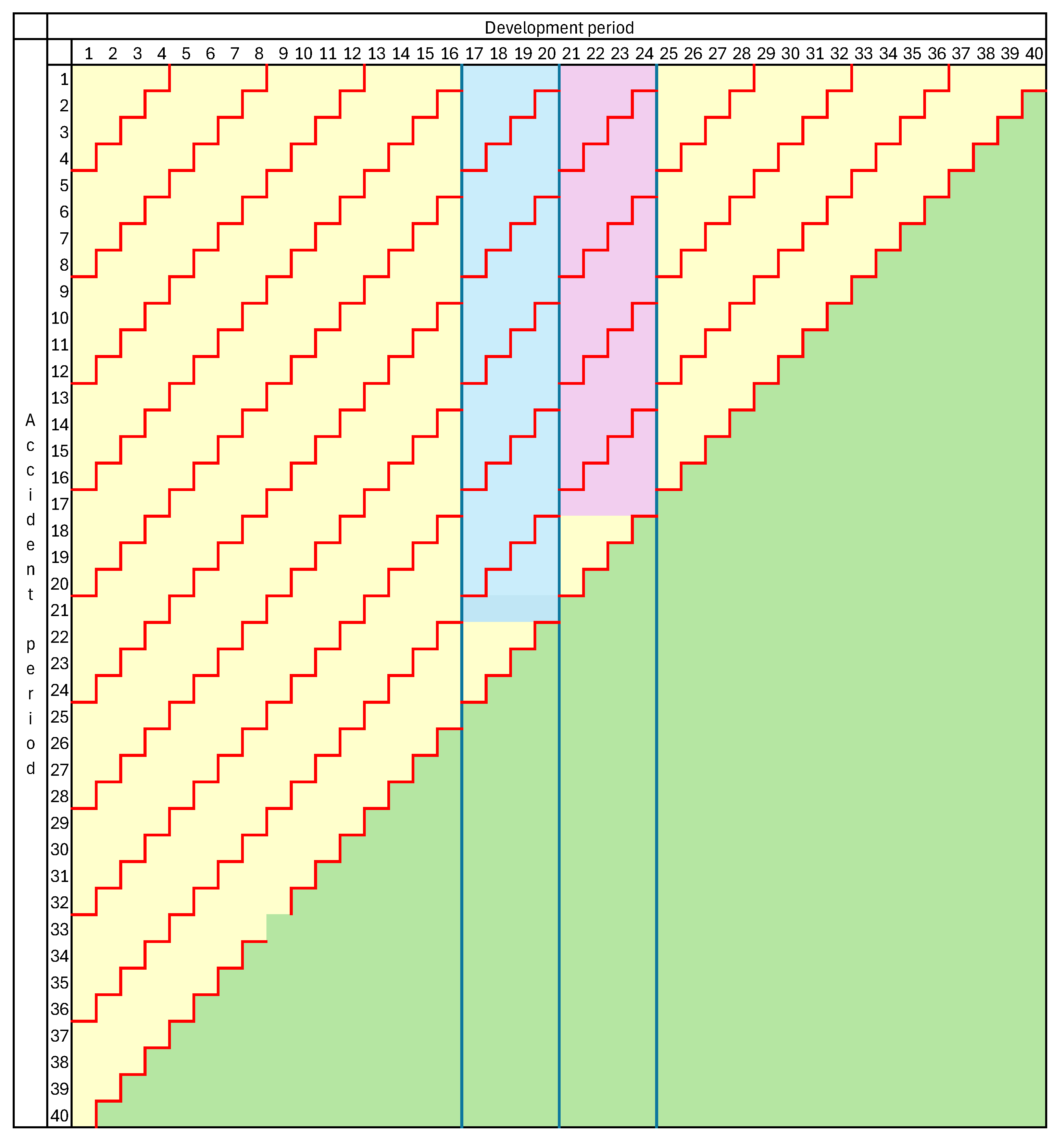
A more general situation is illustrated in Figure 2, where just three cut-points have been inserted, namely ${\omega }_1=16,{\omega }_2=20,{\omega }_3=24.$ This means that development quarters 17 to 20 have been merged into a single development year, here shaded blue, and similarly development quarters 21 to 24, shaded purple. The other development quarters have been left intact. Note that, for each of these development years, there is a triangle of data relating to the latest accident periods. These have not been shaded as they are incomplete and not comparable with the merged development years for earlier accident periods.

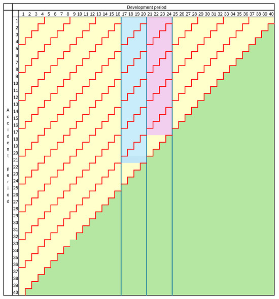
Figure 2. Change of mesh size with preservation of development periods.

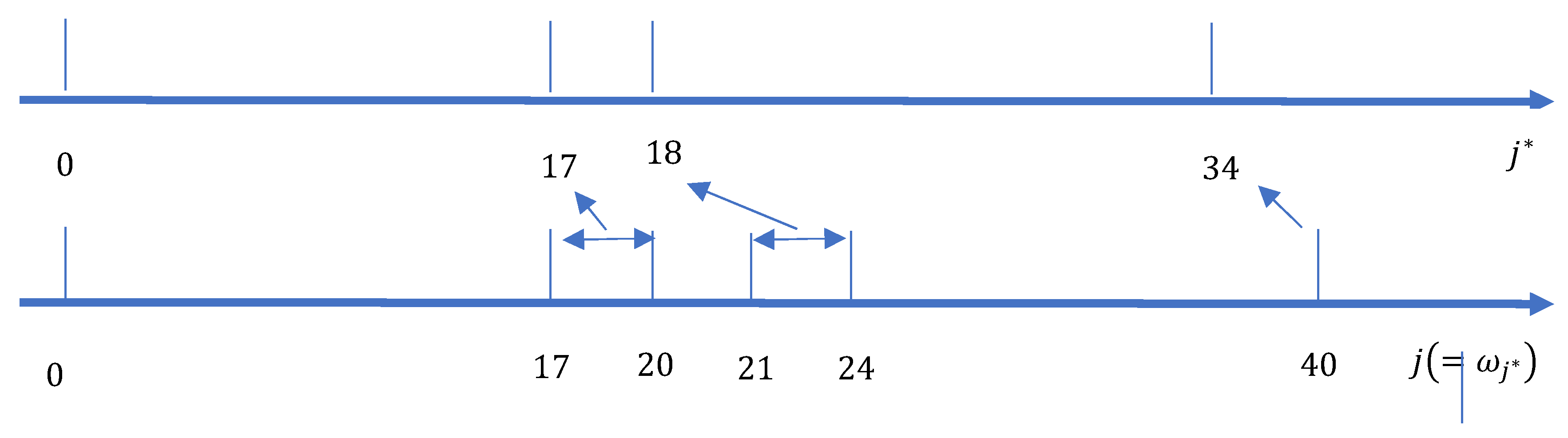
The quantities ${\omega }_{j^{\ast }}$ provide a mapping between the original development periods $j$ and the development periods under the increased mesh size. This is illustrated in Figure 3, which displays the mapping that applies to Figure 2.

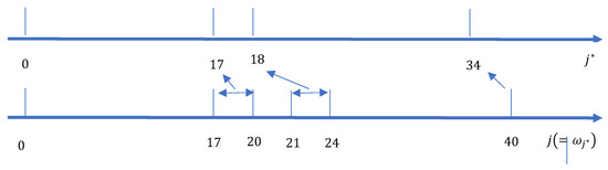
Figure 3. Mapping between original development periods and those under increased mesh size.

In general, let quantities associated with merged development periods be denoted as starred versions of the analogous quantities associated with unmerged development periods. For example, whereas $Y_{ij}$ denotes the claim payments in unmerged development period $j$ of accident period $i$, $Y_{i,k:\mathcal{l}}^{\ast }$ will denote the claim payments in merged development period $k:\mathcal{l}$ of the same accident period, i.e., in development periods $k+1,\dots ,\mathcal{l}$, equivalently, from the end of development period $k$ to the end of development period $\mathcal{l}$.

Greater brevity is possible in denoting cumulative claim payments. Whereas $C_{ij}$ denotes the cumulative claim payments to the end of unmerged development period $j$ of accident period $i$, $C_{ij}^{\ast }$ will denote same quantity, provided that a merged development period ends in the unmerged development period $j$.

Sometimes it will be useful to notate quantities on the merged time scale. For example, $C_{i\left[j^{\ast }\right]}^{\ast }$ will denote cumulative claim payments to the end of the merged development period $j^{\ast }$. Evidently, $C_{i\left[j^{\ast }\right]}^{\ast }=C_{i,{\omega }_{j^{\ast }}}^{\ast }$.

With this adjustment of mesh size, the data set ${\mathcal{D}}_U^{\ast }$ to which a chain ladder will be applied comprises all cells of ${\mathcal{D}}_U$ that form complete development periods under the enlarged mesh. In Figure 2, these are the blue and purple cells for (original) development periods 16 to 23 and the yellow cells for other development periods.

In the general case described earlier in this sub-section,

$${\mathcal{D}}_U^{\ast }=\left\{Y_{i,j:k}^{\ast }:i=1,\dots ,I,j^{\ast } \mathrm{s}\mathrm{u}\mathrm{c}\mathrm{h} \mathrm{t}\mathrm{h}\mathrm{a}\mathrm{t} {j={\omega }_{j^{\ast }-1},k=\omega }_{j^{\ast }}\le I-i+1 \mathrm{f}\mathrm{o}\mathrm{r} \mathrm{s}\mathrm{o}\mathrm{m}\mathrm{e} j^{\ast }\right\},$$

(11)

where

$$Y_{i,j:k}^{\ast }=\sum _{\mathcal{l}={\omega }_{j^{\ast }-1}+1}^{{\omega }_{j^{\ast }}}{Y}_{i\mathcal{l}} .$$

(12)

It is noteworthy that not all rows of ${\mathcal{D}}_U^{\ast }$ extend as far as the $I$-th diagonal of ${\mathcal{D}}_U$. That is to say, the re-constituted data set does not contain all of the most recently available data. It will be useful to construct an indicator of the most recent usable (original) cell of each row. This will be the last cell of the row up to and including the $I$-th diagonal that falls within a complete development period under the enlarged mesh.

Define

$${\tilde{j}}^{\ast }\left(i\right)=max\left\{j^{\ast }:{\omega }_{j^{\ast }}\le I-i+1\right\},$$

(13)

$$\tilde{j}\left(i\right)={\omega }_{{\tilde{j}}^{\ast }\left(i\right)} ,$$

(14)

which is to say that ${\tilde{j}}^{\ast }\left(i\right)$ is the last complete merged development period in row $i$, and $\tilde{j}\left(i\right)$ is the last unmerged development period contained in ${\tilde{j}}^{\ast }\left(i\right)$.

Similarly, define the maximum row containing the complete development period $j^{\ast }$ as

$$\tilde{i}\left(j^{\ast }\right)=max\left\{i:{\omega }_{j^{\ast }}\le I-i+1\right\}.$$

(15)

It will also be useful to define the following quantities, in parallel with $s_j$ and $s_j^{-}$,

$$s_{\left[j^{\ast }\right]}^{\ast }= \sum _{i=1}^{\tilde{i}\left(j^{\ast }\right)}{c}_{i\left[j^{\ast }\right]}^{\ast } ,$$

(16)

$$s_{\left[j^{\ast }\right]}^{\ast -}= \sum _{i=1}^{\tilde{i}\left(j^{\ast }+1\right)}{c}_{i\left[j^{\ast }\right]}^{\ast } .$$

(17)

3. Mack Chain Ladder

3.1. Model Assumptions

Assumption 1

(Mack assumption (1)). $E\left(C_{i,j+1}|C_{i1},\dots ,C_{ij}\right)=C_{ij}{f}_j$ for all $C_{ij}\in \mathcal{D}$ with $j<I$.

The factor $f_j>0$ is usually referred to as an age-to-age factor or a link ratio.

Assumption 2

(Mack assumption (2)). Different accident periods are stochastically independent; i.e., $\left\{C_{i1},\dots ,C_{iI}\right\},\left\{C_{k1},\dots ,C_{kI}\right\}$ are independent for $i\ne k$.

Assumption 3

(Mack assumption (3)). $Var\left(C_{i,j+1}|C_{i1},\dots ,C_{ij}\right)=C_{ij}{\sigma }_j^2$ for all $C_{ij}\in \mathcal{D}$ with $j<I$.

This is the totality of Mack’s assumptions, but it will be convenient to add a few further very mild assumptions here.

Assumption 4.

${\sigma }_j^2>0,j=1,\dots ,I$. This asserts only that no observations are deterministic.

Assumption 5.

$c_{i,I-i+1}>0,i=1,\dots ,I$. The purpose here is to avoid a non-positive forecast of future claims (see (21) below).

Assumption 6.

$s_j^{-}\ne 0,j=1,\dots ,I-1$. The purpose here is to ensure that the chain ladder algorithm is well-defined (see (18) below). It seems that this assumption is implicit in Mack’s paper.

3.2. Estimation of Loss Reserve

The chain ladder proceeds to estimate loss reserve as follows. As given by Mack, the age-to-age factor $f_j$ and dispersion factor ${\sigma }_j^2$ are estimated by

$${\widehat{f}}_j={\displaystyle \frac{s_{j+1}}{s_j^{-}}}$$

(18)

and

$${\widehat{\sigma }}_j^2={\displaystyle \frac{1}{I-j-2}}\sum _{i=1}^{I-j-1}{c}_{ij}{\left(F_{ij}-{\widehat{f}}_j\right)}^2 ,$$

(19)

where

$$F_{ij}={\displaystyle \frac{c_{i,j+1}}{c_{ij}}} .$$

(20)

The forecasts ${\widehat{C}}_{ij}\in {\widehat{\mathcal{D}}}_L$ are then calculated as

$${\widehat{C}}_{ij}=c_{i,I-i+1}{\widehat{f}}_{I-i+1}{\widehat{f}}_{I-i+2}\dots {\widehat{f}}_{j-1}.$$

(21)

As noted in Section 2, $C_{i,I}$ is the ultimate claim cost of accident period $i$, and so ${\widehat{C}}_{i,I}$ is an estimate of this quantity. The amount of outstanding losses for this accident period is equal to

$$R_i=C_{i,I}-c_{i,I-\mathrm{i}+1},$$

(22)

and is estimated by

$${\widehat{R}}_i={\widehat{C}}_{i,I}-c_{i,I-\mathrm{i}+1}.$$

(23)

The total reserve for all accident periods of interest is

$$R=\sum _{i=2}^I{R}_i,$$

(24)

which is estimated by

$$\widehat{R}=\sum _{i=2}^I{\widehat{R}}_i.$$

(25)

Mack derives the following results on the basis of the assumptions of Section 3.1.

Proposition 1

(Mack’s Theorem 2). Under Assumptions 1 and 2, the estimators ${\widehat{f}}_j,j=1,\dots ,I-1$ are unbiased and uncorrelated. It follows that ${\widehat{R}}_i$ is an unbiased estimator of $R_i$.

3.3. Variance of Forecast

It will be convenient to introduce the notation

$$F_{i,\mathcal{l}:m}=F_{i\mathcal{l}}{F}_{i,\mathcal{l}+1}\dots F_{i,m-1},$$

(26)

$$F_{\mathcal{l}:m}=f_{\mathcal{l}}{f}_{\mathcal{l}+1}\dots f_{m-1},$$

(27)

$${\widehat{F}}_{\mathcal{l}:m}={\widehat{f}}_{\mathcal{l}}{\widehat{f}}_{\mathcal{l}+1}\dots {\widehat{f}}_{m-1},$$

(28)

subject to the convention that $F_{i,\mathcal{l}:m}=F_{\mathcal{l}:m}={\widehat{F}}_{\mathcal{l}:m}=1$ for $\mathcal{l}\ge m$.

Remark 1.

It will be found useful later to remark that $F_{\mathcal{l}:m}>0$, which follows from the fact that $f_j>0$ in Assumption 1.

The variance of the estimated reserve ${\widehat{R}}_i$ is of interest, specifically $Var\left[{\widehat{R}}_i|{\mathcal{D}}_U\right]=Var\left[{\widehat{C}}_{iI}-c_{i,I-\mathrm{i}+1}|{\mathcal{D}}_U\right]=Var\left[{\widehat{C}}_{iI}|{\mathcal{D}}_U\right]=Var\left[c_{i,I-i+1}{\widehat{F}}_i|{\mathcal{D}}_U\right]$, where ${\widehat{F}}_i$ is the further abbreviation ${\widehat{F}}_i={\widehat{F}}_{I-i+1:I}$.

It will be convenient to write

$$Var\left[{\widehat{R}}_i^k|{\mathcal{D}}_U\right]={\left(C_{iI}^k\right)}^2{V}_i^k,$$

(29)

where ${\widehat{R}}_i^k$ denotes the estimate of $R_i$ with $C_{iI}$ forecast by ${\widehat{C}}_{iI}^k$ on the basis of data to the end of the development period $k\left(\le I-i+1\right)$, i.e.,

$${\widehat{R}}_i^k={\widehat{C}}_{iI}^k-c_{i,\mathrm{I}-\mathrm{i}+1}=c_{i\mathrm{k}}{\widehat{F}}_{k:I}-c_{i,\mathrm{I}-\mathrm{i}+1},$$

(30)

and where

$$C_{iI}^k=c_{ik}{F}_{k:I},$$

(31)

and the addition of a hat has the usual meaning.

Accident period $i$ has developed as far as development period $I-i+1$, and so the estimate of loss reserve that maximizes the use of data is the one appearing in (23), which may be expressed as ${\widehat{R}}_i^{I-i+1}$, and its variance, from (29), is

$$Var\left[{\widehat{R}}_i^{I-i+1}|{\mathcal{D}}_U\right]={\left(C_{iI}^{I-i+1}\right)}^2{V}_i^{I-i+1}.$$

(32)

This (or, more precisely, an estimate of it) was calculated by Mack (1993, p. 217) and also by Gisler (2019, p. 806). Wüthrich and Merz (2008, pp. 53–54) reproduce the same quantity, though they go on to suggest alternative results based on varying bootstrap re-sampling strategies.

The following reconciles with Mack’s result in the case $k=I-i+1$, and extends it to general $k$. The extension follows straightforwardly from the algebra in Mack’s paper dealing with the special case.

$$V_i^k=\sum _{j=k}^{I-1}{\displaystyle \frac{{\sigma }_j^2}{f_j^2}}\left({\displaystyle \frac{1}{c_{i,k}{F}_{k:j}}}+{\displaystyle \frac{1}{s_j^{-}}}\right),$$

(33)

which may be conveniently abbreviated as follows:

$$V_i^k=\sum _{j=k}^{I-1}\left(B_{ijk}+{\displaystyle \frac{{\sigma }_j^2}{f_j^2}}{\displaystyle \frac{1}{s_j^{-}}}\right),$$

(34)

where

$$B_{ijk}={\displaystyle \frac{{\sigma }_j^2}{f_j^2}}{\displaystyle \frac{1}{c_{ik}{F}_{k:j}}} .$$

(35)

There is a recurrence relation that relates values of $V_i^k$ for consecutive evaluation points $k$ and is useful for the computation of these quantities. It is proven in Appendix A.1, and set out in the following.

Proposition 2.

With $V_i^k$ defined by (33), the following recurrence relation holds.

$$V_i^{k-1}=\left(B_{i,k-1,k-1}+{\displaystyle \frac{{\sigma }_{k-1}^2}{f_{k-1}^2}}{\displaystyle \frac{1}{s_{k-1}^{-}}}\right)+\left(1-{\gamma }_{i,k-1}\right)\sum _{j=k}^{I-1}{\displaystyle \frac{{\sigma }_j^2}{f_j^2}}{\displaystyle \frac{1}{s_j^{-}}}+{\gamma }_{i,k-1}{V}_i^k,$$

(36)

where

$${\gamma }_{ik}={\displaystyle \frac{F_{ik}}{f_k}} .$$

(37)

The ratio ${\gamma }_{i,k-1}$ appearing here plays a crucial role in the following and is of interest. The numerator is the observed development of the accident period $i$ from the end of development period $k-1$ to $k$, and the denominator is its expected value. So, for example, ${\gamma }_{i,k-1}>1$ indicates that development over that period exceeds expected.

It is sometimes useful to introduce the parameter ${\varphi }_j={\sigma }_j^2/f_j$. Then, (34) takes the form

$$V_i^k=\sum _{j=k}^{I-1}{\varphi }_j\left({\tilde{B}}_{ijk}+{\displaystyle \frac{1}{f_j}}{\displaystyle \frac{1}{s_j^{-}}}\right),$$

(38)

where

$${\tilde{B}}_{ijk}={\displaystyle \frac{1}{f_j}}{\displaystyle \frac{1}{c_{ik}{F}_{k:j}}}={\displaystyle \frac{1}{c_{ik}{F}_{k:j+1}}} .$$

(39)

An interesting case of (33) occurs when the ratio ${\varphi }_j$ is independent of $j$, which includes the case where all cells of $\mathcal{D}$ are subject to over-dispersed Poisson distributions with common scale parameter. The value of $V_i$ is then given by the following result.

Proposition 3.

Consider the case in which the following assumption holds in addition to Assumptions 1 to 6.

Assumption 7.

${\sigma }_j^2/f_j=\varphi ,$ const. for all $C_{ij}\in \mathcal{D}$.

Then (38) reduces to

$$V_i^k=\varphi \sum _{j=k}^{I-1}\left({\tilde{B}}_{ijk}+{\displaystyle \frac{1}{f_j}}{\displaystyle \frac{1}{s_j^{-}}}\right),$$

(40)

Now consider the total reserve $\widehat{R}$, with each accident period $i$ evaluated at the end of calendar period $I$, i.e., development period $I-i+1$ and ${\widehat{R}}_i={\widehat{R}}_i^{I-i+1}$. By Assumption 2, (25) and (29) yield

$$\begin{array}{l}Var\left[\widehat{R}|{\mathcal{D}}_U\right]=Var\left[{\displaystyle \sum _{i=2}^I}{\widehat{R}}_i^{I-i+1}|{\mathcal{D}}_U\right]\\ ={\displaystyle \sum _{i=2}^I}{\left(C_{iI}^{I-i+1}\right)}^2{V}_i^{I-i+1}+2\sum _{\begin{array}{c}i,k=2\\ i<k\end{array}}^I{c}_{i,I-i+1}{c}_{k,I-k+1}Cov\left[{\widehat{F}}_i{,\widehat{F}}_k|{\mathcal{D}}_U\right].\end{array}$$

(41)

where, in the last summation, the summand draws on (21).

This may be simplified by taking account of Proposition 1. The covariance term becomes (remembering that $i<k$)

$$\begin{array}{l}Cov\left[{\widehat{F}}_i{,\widehat{F}}_k|{\mathcal{D}}_U\right]=Cov\left[{\widehat{F}}_i{,{\widehat{F}}_{k,I-k+1:I-i+1}\widehat{F}}_i|{\mathcal{D}}_U\right]=E\left[{\widehat{F}}_{k,I-k+1:I-i+1}\right]Var\left[{\widehat{F}}_i|{\mathcal{D}}_U\right]\\ =F_{I-k+1:I-i+1}{\left({\displaystyle \frac{C_{iI}^{I-i+1}}{c_{i,I-i+1}}}\right)}^2{V}_i^{I-i+1} ,\end{array}$$

(42)

where the second equality follows from Proposition 1 and the last equality from (29) and (30). With substitution of (42), result (41) becomes

$$\begin{array}{l}Var\left[\widehat{R}|{\mathcal{D}}_U\right]={\displaystyle \sum _{i=2}^I}{\left(C_{iI}^{I-i+1}\right)}^2{V}_i^{I-i+1}\\ +2{\displaystyle \sum _{\begin{array}{c}i,k=2\\ i<k\end{array}}^I}{c}_{i,I-i+1}{c}_{k,I-k+1}{F}_{k,I-k+1:I-i+1}{\left({\displaystyle \frac{C_{iI}^{I-i+1}}{c_{i,I-i+1}}}\right)}^2{V}_i^{I-i+1}\\ ={\displaystyle \sum _{i=2}^I}{\left(C_{iI}^{I-i+1}\right)}^2{V}_i^{I-i+1}\left(1+2{\displaystyle \sum _{k=i+1}^I}{\displaystyle \frac{c_{k,I-k+1}}{c_{i,I-i+1}}}{F}_{k,I-k+1:I-i+1}\right)\\ ={\displaystyle \sum _{i=2}^I}{\left(C_{iI}^{I-i+1}\right)}^2{V}_i^{I-i+1}\left({\displaystyle \sum _{k=2}^I}{\displaystyle \frac{C_{k,I-i+1}}{c_{i,I-i+1}}}\right).\end{array}$$

(43)

4. Effect of Change of Mesh Size Under the Preservation of Development Periods

Section 2.2 discussed two types of change of mesh size, preserving, respectively, calendar and development periods. These two types of change carry very different implications for chain ladder models. The effects of both types of change on the EDF chain ladder were discussed by Taylor (2025).

It is also necessary to consider the effects of both on the Mack chain ladder. This, however, would expand the present paper beyond a reasonable size. For this reason, the following sections consider only changes in mesh that preserve development periods. The preservation of calendar periods may be considered in a separate paper.

A forerunner to the examination of the effects of change of mesh size under the preservation of development periods is a consideration of whether or not the Mack chain ladder structure is maintained under such changes. This will be the subject of Section 4.1.

4.1. Maintenance of Model Assumptions

4.1.1. Cell Means

Consider the change of mesh described in Section 2.2.2. The notation will be as introduced there. For brevity, just label the merged development periods $j^{\ast }=0,\dots ,J^{\ast }-1$. It is necessary to check whether the Mack chain ladder model is applicable under the changed mesh size, i.e., whether Assumptions 1 to 6 of Section 3.1 continue to hold. The present sub-section examines Assumptions 1, 2, 5 and 6; the next examines Assumptions 3 and 4.

• Discussion of Assumption 1

Consider a generic merged development period $j^{\ast }+1{\equiv \omega }_{j^{\ast }}{:\omega }_{j^{\ast }+1}$. According to the notation of Section 2.2.2,

$$E\left(C_{i\left[j^{\ast }+1\right]}^{\ast }|C_{i1}^{\ast },\dots ,C_{i\left[j^{\ast }\right]}^{\ast }\right)=\sum _{k={\omega }_{j^{\ast }}+1}^{{\omega }_{j^{\ast }+1}}E\left(C_{ik}|C_{i1}^{\ast },\dots ,C_{i\left[j^{\ast }\right]}^{\ast }\right) ,$$

(44)

Now, for $k\ge {\omega }_{j^{\ast }}$,

$$\begin{array}{l}E\left(C_{ik}|C_{i1}^{\ast },\dots ,C_{i\left[j^{\ast }\right]}^{\ast }\right)=E\left(C_{i,k-1}{f}_{k-1}|C_{i1}^{\ast },\dots ,C_{i\left[j^{\ast }\right]}^{\ast }\right)\\ =E\left(C_{i,k-2}{f}_{k-2}{f}_{k-1}|C_{i1}^{\ast },\dots ,C_{i\left[j^{\ast }\right]}^{\ast }\right)=\dots =C_{i\left[j^{\ast }\right]}^{\ast }{F}_{{\omega }_{j^{\ast }}:k},\end{array}$$

(45)

By the repeated application of Assumption 1.

Substitution of (45) into (44) then yields

$$E\left(C_{i\left[j^{\ast }+1\right]}^{\ast }|C_{i1}^{\ast },\dots ,C_{i\left[j^{\ast }\right]}^{\ast }\right)=C_{i\left[j^{\ast }\right]}^{\ast }\sum _{k={\omega }_{j^{\ast }}+1}^{{\omega }_{j^{\ast }+1}}{F}_{{\omega }_{j^{\ast }}:k} ,$$

(46)

which is of the form required by Assumption 1, and so this form of assumption continues to hold for the enlarged mesh size.

• Discussion of Assumption 2

Note that $\left\{C_{i{\omega }_1}^{\ast },\dots ,C_{i{\omega }_{J^{\ast }}}^{\ast }\right\}$ is a subset of $\left\{C_{i1},\dots ,C_{iI}\right\}.$ It then follows from Assumption 2 that $\left\{C_{i{\omega }_1}^{\ast },\dots ,C_{i{\omega }_{J^{\ast }}}^{\ast }\right\},\left\{C_{ik}^{\ast },\dots ,C_{k{\omega }_{J^{\ast }}}^{\ast }\right\}$ are independent for $i\ne k$. This is of the same form as Assumption 2, and so this form of assumption continues to hold for the enlarged mesh size.

• Discussion of Assumption 5

With the change of mesh size, this assumption requires replacement by the following.

Assumption 5*.

$c_{i,\tilde{j}\left(i\right)}^{\ast }>0,i=1,\dots ,I$.

• Discussion of Assumption 6

With the change of mesh size, this assumption requires replacement by the following.

Assumption 6*.

$s_{j^{\ast }}^{\ast -}\ne 0,j^{\ast }=1,\dots ,J^{\ast }-1$.

4.1.2. Cell Variances

• Discussion of Assumption 3

Mack (1993, Theorem 3) evaluates variances of the form $Var\left[C_{iI}|C_{i1},\dots ,C_{ij}\right]$, and the calculation given there is easily adapted to the case $Var\left[\left(C_{ik}\right)|C_{i1},\dots ,C_{ij}\right]$ for $j<k\le I$. The result is

$$Var\left(C_{ik}|C_{i1},\dots ,C_{ij}\right)=C_{ij}\sum _{\mathcal{l}=j}^{k-1}{f}_j\dots f_{\mathcal{l}-1}{\sigma }_{\mathcal{l}}^2{f}_{\mathcal{l}+1}^2\dots f_{k-1}^2.$$

(47)

Simple adaptation to the present situation yields

$$Var\left(C_{i\left[j^{\ast }+1\right]+1}^{\ast }|C_{i0}^{\ast },\dots ,C_{i\left[j^{\ast }\right]}^{\ast }\right)=C_{i\left[j^{\ast }\right]}^{\ast }\sum _{\mathcal{l}={\omega }_{j^{\ast }}}^{{\omega }_{j^{\ast }+1}-1}{f}_{{\omega }_{j^{\ast }}}\dots f_{\mathcal{l}-1}{\sigma }_{\mathcal{l}}^2{f}_{\mathcal{l}+1}^2\dots f_{{\omega }_{j^{\ast }+1}-1}^2 .$$

(48)

This can be expressed in the form

$$Var\left(C_{i\left[j^{\ast }+1\right]}^{\ast }|C_{i0}^{\ast },\dots ,C_{i\left[j^{\ast }\right]}^{\ast }\right)=C_{i\left[j^{\ast }\right]}^{\ast }{\sigma }_{\left[j^{\ast }\right]}^{\ast 2}$$

(49)

where

$${\sigma }_{\left[j^{\ast }\right]}^{\ast 2}=\sum _{\mathcal{l}={\omega }_{j^{\ast }}}^{{\omega }_{j^{\ast }+1}-1}{f}_{{\omega }_{j^{\ast }}}\dots f_{\mathcal{l}-1}{\sigma }_{\mathcal{l}}^2{f}_{\mathcal{l}+1}^2\dots f_{{\omega }_{j^{\ast }+1}-1}^2 .$$

(50)

The relation (49) is of the form required by Assumption 3, which therefore continues to hold for the enlarged mesh size.

• Discussion of Assumption 4

By Assumptions 1 and 3, $f_j,{\sigma }_j^2>0$, and it immediately follows from (50) that ${\sigma }_{\left[j^{\ast }\right]}^{\ast 2}>0$, as required by Assumption 4.

The reasoning of Section 4.1.1 and the present sub-section leads to the following result.

Proposition 4.

Consider the data array $\mathcal{D}$, and suppose it is subject to a Mack chain ladder model in the sense of satisfying Assumptions 1 to 6 of Section 3.1. Now impose the change of mesh size described in Section 2.2.2. This induces new data sets ${\mathcal{D}}_U^{\ast },{\mathcal{D}}_L^{\ast }$ and ${{\mathcal{D}}^{\ast }=\mathcal{D}}_U^{\ast }\cup {\mathcal{D}}_L^{\ast }$. If Assumptions 5 and 6, are replaced by 5* and 6*, then ${\mathcal{D}}^{\ast }$ will also be subject to a Mack chain ladder model.

4.1.3. Estimation of Loss Reserve

The estimation proceeds in parallel with Section 3.2. In place of (18) to (20), one writes

$${\widehat{f}}_{\left[j^{\ast }\right]}^{\ast }={\displaystyle \frac{s_{\left[j^{\ast }+1\right]}^{\ast }}{s_{\left[j^{\ast }\right]}^{\ast -}}} , j^{\ast }=1,\dots , J^{\ast }-1,$$

(51)

and

$${\widehat{\sigma }}_{\left[j^{\ast }\right]}^{\ast 2}={\displaystyle \frac{1}{\tilde{i}\left(j^{\ast }\right)-2}}\sum _{i=1}^{\tilde{i}\left(j^{\ast }\right)-1}{c}_{i\left[j^{\ast }\right]}^{\ast }{\left(F_{i\left[j^{\ast }\right]}^{\ast }-{\widehat{f}}_{\left[j^{\ast }\right]}^{\ast }\right)}^2 , j^{\ast }=1,\dots , J^{\ast }-2.$$

(52)

where

$$F_{i\left[j^{\ast }\right]}^{\ast }={\displaystyle \frac{c_{i\left[j^{\ast }+1\right]}^{\ast }}{c_{i\left[j^{\ast }\right]}^{\ast }}} .$$

(53)

The forecasts ${\widehat{C}}_{i\left[k^{\ast }\right]}^{\ast }$ are calculated as

$${\widehat{C}}_{i\left[k^{\ast }\right]}^{\ast }=c_{i\left[{\tilde{j}}^{\ast }\left(i\right)\right]}^{\ast }{\widehat{f}}_{\left[{\tilde{j}}^{\ast }\left(i\right)\right]}^{\ast }{\widehat{f}}_{\left[{\tilde{j}}^{\ast }\left(i\right)+1\right]}^{\ast }\dots {\widehat{f}}_{\left[k^{\ast }-1\right]}^{\ast },k^{\ast }={\tilde{j}}^{\ast }\left(i\right)+1,{\tilde{j}}^{\ast }\left(i\right)+2,\dots ,J^{\ast }.$$

(54)

With an obvious notation parallel to (26)–(28), this last forecast may be abbreviated as follows:

$${\widehat{C}}_{i\left[k^{\ast }\right]}^{\ast }=c_{i\left[{\tilde{j}}^{\ast }\left(i\right)\right]}^{\ast }{\widehat{F}}_{\left[{\tilde{j}}^{\ast }\left(i\right):k^{\ast }\right]}^{\ast },k^{\ast }={\tilde{j}}^{\ast }\left(i\right)+1,{\tilde{j}}^{\ast }\left(i\right)+2,\dots ,J^{\ast }.$$

(55)

The forecast ultimate claim cost of accident period $i$ is then

$${{\widehat{C}}_{iI}^{\ast }=\widehat{C}}_{i\left[J^{\ast }\right]}^{\ast }=c_{i\left[{\tilde{j}}^{\ast }\left(i\right)\right]}^{\ast }{\widehat{F}}_{\left[{\tilde{j}}^{\ast }\left(i\right):J^{\ast }\right]}^{\ast }.$$

(56)

Corresponding to (23) is

$${\widehat{R}}_i^{\ast }={\widehat{C}}_{i\left[J^{\ast }\right]}^{\ast }-{\mathrm{c}}_{i,I-i+1},$$

(57)

and (25) follows as previously. Note here that the value of ${\mathrm{c}}_{i,I-i+1}$ is known (it is the total amount of claims paid to the valuation date in respect of accident period $i$) though it is not usable in the estimation of an age-to-age factor.

The forecasts in (54) are based on the data point $c_{i\left[{\tilde{j}}^{\ast }\left(i\right)\right]}^{\ast }$, and, as noted in Section 2.2.2, this does not always coincide with the most recent data point $c_{i,I-i+1}$ under the original mesh size. Definition (13) shows that, when it does not, ${\omega }_{j^{\ast }}<I-i+1$, meaning that development period ${\tilde{j}}^{\ast }\left(i\right)$ does not include data from the $I$-th diagonal of ${\mathcal{D}}_U$. The consequence of this is as follows.

Proposition 5.

When an increase in mesh size converts data triangle ${\mathcal{D}}_U$ to ${\mathcal{D}}_U^{\ast }$, and a chain ladder model is applied to ${\mathcal{D}}_U^{\ast }$ in accordance with Section 4.1.1, the forecasts (54) for some accident periods will rely on earlier data than was available for the same accident periods in ${\mathcal{D}}_U$.

Nevertheless, the following can be said of this model’s forecasts, in parallel with Proposition 1. The reasoning is the same as there.

Proposition 6.

Under Assumptions 1 and 2, the estimators ${\widehat{f}}_{\left[j^{\ast }\right]}^{\ast },j^{\ast }=1,\dots , J^{\ast }-1$ are unbiased and uncorrelated. It follows that ${\widehat{R}}_i^{\ast }$ is an unbiased estimator of $R_i^{\ast }$.

4.2. Forecast Variance

4.2.1. Variation of Mesh over Development Periods

It will be convenient to commence with a consideration of the case in which an enlargement of mesh size is effected by the coalescence of just two consecutive development periods, say $j^{†}$ and $j^{†}+1$. In the notation of Section 2.2.2, $\left\{1,\dots ,I\right\}$ is partitioned into the $I-1$ subsets by cut-points ${\omega }_{j^{\ast }}=j^{\ast }$ for $j^{\ast }=\mathrm{0,1},\dots , j^{†}-1$ and ${\omega }_{j^{\ast }}=j^{\ast }+1$ for $j^{\ast }= j^{†},\dots ,I-1$.

In this case, (13) and (15) yield

$$\begin{gathered} {\tilde{j}}^{\ast }\left(i\right)=I-i+1,i>I-j^{†}+1 \\ =I-i,i\le I-j^{†}+1 \end{gathered}$$

(58)

and

$$\begin{gathered} \tilde{i}\left(j^{\ast }\right)=I-j^{\ast }+1,j^{\ast }<j^{†} \\ =I-j^{\ast },j^{\ast }\ge j^{†}. \end{gathered}$$

(59)

The variance of loss reserve estimate in (29) and (33) is now replaced by the following.

$$Var\left[{\widehat{R}}_i^{\left[k\right]\ast }|{\mathcal{D}}_U^{\ast }\right]={\left(C_{iI}^{\left[k\right]\ast }\right)}^2{V}_i^{\left[k\right]\ast }.$$

(60)

where $V_i^{\left[k\right]\ast }$ is yet to be determined and is the quantity corresponding to $V_i^k$ in (33) when development periods $j^{†}$ and $j^{†}+1$ are merged, as above.

To calculate how $V_i^{\ast }$ differs from $V_i$, it is necessary to consider three cases as follows.

Case I: $i<I-j^{†}+1$. In this case $I-i+1>j^{†}$, which means that past development includes the two merged development periods $j^{†},j^{†}+1$, and so accident period $i$ will in the future pass through only development periods with “normal” age-to-age factors. It also follows from (58) that ${\tilde{j}}^{\ast }\left(i\right)=I-i$, which corresponds with $j=I-i+1$.

Case II: $i>I-j^{†}+1$. In this case $I-i+1<j^{†}$, which means that past development has not yet reached development period $j^{†}$, the first of the two to be merged, and so the accident period $i$ will in the future pass through both development periods $j^{†},j^{†}+1$. It also follows from (58) that ${\tilde{j}}^{\ast }\left(i\right)=I-i+1,\mathrm{w}\mathrm{h}\mathrm{i}\mathrm{c}\mathrm{h} \mathrm{c}\mathrm{o}\mathrm{r}\mathrm{r}\mathrm{e}\mathrm{s}\mathrm{p}\mathrm{o}\mathrm{n}\mathrm{d}\mathrm{s} \mathrm{w}\mathrm{i}\mathrm{t}\mathrm{h} j=I-i+1$.

Case III: $i=I-j^{†}+1$. In this case $I-i+1=j^{†}$, which means that past development has passed through the first of the “abnormal” development periods, $j^{†}$, but not the second, $j^{†}$+1. It may be noted that the merged cell $\left(I-j^{†}+1,\left[j^{†}\right]\right)$ is incomplete, since the unmerged cell $\left(I-j^{†}+1,j^{†}+1\right)$ lies in the future. It also follows from (58) that ${\tilde{j}}^{\ast }\left(i\right)=I-i$, which corresponds with $j=I-i$.

It is evident from the description of Case I that, the data point $c_{i,I-i+1}$ is available in row $i$, and the variance of the estimated loss reserve may be calculated in the “normal” way. Specifically, (60) may be applied with $k=I-i$:

$$Var\left[{\widehat{R}}_i^{\left[I-i\right]\ast }|{\mathcal{D}}_U^{\ast }\right]={\left(C_{iI}^{\left[I-i\right]\ast }\right)}^2{V}_i^{\left[I-i\right]\ast }={\left(C_{iI}^{I-i+1}\right)}^2{V}_i^{I-i+1},$$

(61)

with the last two terms on the right obtained from (60) and (61).

Case II may be dealt with similarly, and again (61) arises. The fact that accident period $i$ is still to pass through the two merged development periods $j^{†},j^{†}+1$ has no effect on the stochastic behavior of the variance.

Case III is a little different. Here (61) is replaced by

$$Var\left[{\widehat{R}}_i^{\left[I-i\right]\ast }|{\mathcal{D}}_U^{\ast }\right]={\left(C_{iI}^{\left[I-i\right]\ast }\right)}^2{V}_i^{\left[I-i\right]\ast }={\left(C_{iI}^{I-i}\right)}^2{V}_i^{I-i}={\left(C_{I-j^{†}+1,I}^{j^{†}-1}\right)}^2{V}_{I-j^{†}+1}^{j^{†}-1}.$$

(62)

In this case, the data point $c_{I-j^{†}+1,j^{†}}$ must be forfeited as it forms part of an incomplete merged cell, and so the valuation standpoint must be taken at the end of the development period $I-i$ instead of the usual $I-i+1$.

The following proposition summarizes the situation.

Proposition 7.

With $V_i^k$ defined by (34), the relevant variances of loss reserve estimates are the following:

• For $i<I-j^{†}+1,Var\left[{\widehat{R}}_i^{\left[I-i\right]\ast }|{\mathcal{D}}_U^{\ast }\right]={\left(C_{iI}^{I-i+1}\right)}^2{V}_i^{I-i+1} ,$
• For $i>I-j^{†}+1,Var\left[{\widehat{R}}_i^{\left[I-i+1\right]\ast }|{\mathcal{D}}_U^{\ast }\right]={\left(C_{iI}^{I-i+1}\right)}^2{V}_i^{I-i+1} ,$
• For $i=I-j^{†}+1,Var\left[{\widehat{R}}_i^{\left[I-i\right]\ast }|{\mathcal{D}}_U^{\ast }\right]={\left(C_{I-j^{†}+1,I}^{j^{†}-1}\right)}^2{V}_{I-j^{†}+1}^{j^{†}-1} .$

It is evident from this result and (29) that the variance of estimated loss reserve is unchanged by the merger of the two development periods for all $i\ne I-j^{†}+1$. However, this equality does not hold for $i=I-j^{†}+1$, and the question of interest concerns the relative magnitudes of $Var\left[{\widehat{R}}_i^{\left[I-i\right]\ast }|{\mathcal{D}}_U^{\ast }\right] \mathrm{a}\mathrm{n}\mathrm{d} Var\left[{\widehat{R}}_i^{I-i+1}|{\mathcal{D}}_U\right]$.

To study this question, one can write

$$\begin{array}{l}Var\left[{\widehat{R}}_i^{\left[I-i\right]\ast }|{\mathcal{D}}_U^{\ast }\right]-Var\left[{\widehat{R}}_i^{I-i+1}|{\mathcal{D}}_U\right]\\ ={\left(C_{I-j^{†}+1,I}^{j^{†}-1}\right)}^2{V}_{I-j^{†}+1}^{j^{†}-1}-{\left(C_{I-j^{†}+1,I}^{j^{†}}\right)}^2{V}_{I-j^{†}+1}^{j^{†}}.\end{array}$$

(63)

Define

$${\pi }_i^k={\displaystyle \frac{\sum _{j=k}^{I-1}{B}_{ijk}}{\sum _{j=k}^{I-1}{B}_{ijk}+\sum _{j=k}^{I-1}\frac{{\sigma }_j^2}{f_j^2}\frac{1}{s_j^{-}}}}={\displaystyle \frac{\sum _{j=k}^{I-1}{B}_{ijk}}{V_i^k}} ,$$

(64)

and note that

$${1-\pi }_i^k={\displaystyle \frac{\sum _{j=k}^{I-1}\frac{{\sigma }_j^2}{f_j^2}\frac{1}{s_j^{-}}}{\sum _{j=k}^{I-1}{B}_{ijk}+\sum _{j=k}^{I-1}\frac{{\sigma }_j^2}{f_j^2}\frac{1}{s_j^{-}}}}={\displaystyle \frac{\sum _{j=k}^{I-1}\frac{{\sigma }_j^2}{f_j^2}\frac{1}{s_j^{-}}}{V_i^k}} ,$$

(65)

And

$$V_i^k-\sum _{j=k}^{I-1}{\displaystyle \frac{{\sigma }_j^2}{f_j^2}}{\displaystyle \frac{1}{s_j^{-}}}=\sum _{j=k}^{I-1}{B}_{ijk} ,$$

(66)

where (34) has been used to obtain the last three relations.

It is evident from (64) that

$${0<\pi }_i^k<1 .$$

(67)

The following result, proven in Appendix A.2, establishes the ordering of $Var\left[{\widehat{R}}_i^{\ast }|{\mathcal{D}}_U^{\ast }\right] \mathrm{a}\mathrm{n}\mathrm{d} Var\left[{\widehat{R}}_i|{\mathcal{D}}_U\right]$.

Proposition 8.

For the case $i=I-j^{†}+1$, a necessary and sufficient condition that $Var\left[{\widehat{R}}_i^{\ast }|{\mathcal{D}}_U^{\ast }\right]>(=,<)Var\left[{\widehat{R}}_i|{\mathcal{D}}_U\right]$ is

$${{\gamma }_{i,k-1}<\left(=,>\right)\gamma }_{i,k-1}^0 ,$$

(68)

where ${k=j}^{†}$ and the threshold value ${\gamma }_{i,k-1}^0$ is given by

$${\gamma }_{i,k-1}^0= {½\pi }_i^k+{\left(1-½{\pi }_i^k\right)\left(1+{\displaystyle \frac{{\omega }_{i,k-1}}{{\left(1-½{\pi }_i^k\right)}^2}}\right)}^{½}.$$

(69)

with

$${\omega }_{i,k-1}={\displaystyle \frac{B_{i,k-1,k-1}+\frac{{\sigma }_{k-1}^2}{f_{k-1}^2}\frac{1}{s_{k-1}^{-}}}{V_i^k}} .$$

(70)

Corollary 1.

It follows from (70) that ${\gamma }_{i,k-1}^0>1$, and so a sufficient condition that $Var\left[{\widehat{R}}_i^{\ast }|{\mathcal{D}}_U^{\ast }\right]>Var\left[{\widehat{R}}_i|{\mathcal{D}}_U\right]$ is that ${\gamma }_{i,k-1}<1, i.e. F_{i,k-1}<f_{k-1}$, where $i,k$ take the same values as in Proposition 8.

The main conclusion to be drawn from Proposition 8 is that $Var\left[{\widehat{R}}_i^{\ast }|{\mathcal{D}}_U^{\ast }\right]$ does not always exceed $Var\left[{\widehat{R}}_i|{\mathcal{D}}_U\right]$. That is to say, the merger of development periods (or decreasing granularity) does not always result in increased predictive variance. This result differs from the corresponding one for the EDF chain ladder in Taylor (2025).

The difference arises from the unique feature of the Mack chain ladder according to which the variance of predicted loss reserve is conditioned by, and in fact is proportional to, the squared amount of claims paid to the date of valuation (see (32)). It is seen above that when development periods $j^{†}$ and $j^{†}+1$ are merged, the estimated variance of forecast loss reserve accident for accident period $i=I-j^{†}+1$ becomes proportional to $c_{i,I-i}$ instead of $c_{i,I-i+1}$.

If $c_{i,I-i}$ is small relative to $c_{i,I-i+1}$, then it can turn out that $Var\left[{\widehat{R}}_i^{\ast }|{\mathcal{D}}_U^{\ast }\right]<Var\left[{\widehat{R}}_i|{\mathcal{D}}_U\right]$. This is precisely what happens when $F_{i,I-i}=c_{i,I-i+1}/c_{i,I-i}$ is larger than its expected value $f_{I-i}$ by a sufficient margin.

Corollary 1 points out that the threshold value ${\gamma }_{i,k-1}^0>1$, and, to this extent, $Var\left[{\widehat{R}}_i^{\ast }|{\mathcal{D}}_U^{\ast }\right]$ will tend to exceed $Var\left[{\widehat{R}}_i|{\mathcal{D}}_U\right]$; i.e., decreasing granularity will tend to lead to increased variance of loss reserve forecast, but not invariably.

A numerical example of these thresholds is now given. It is based on the numerical example from Mack (1993), which in turn uses the data set from Taylor and Ashe (1983). The data set is reproduced in Appendix B.

The parameter estimates of $f_j$ and ${\sigma }_j^2$ given by Mack just after his Table 1, after mild smoothing, are taken as parameters for the purpose of this example and are displayed in Table 1 below.

Table 1. Mack chain ladder parameters.

$\mathit{j}$	${\mathit{f}}_{\mathit{j}}$	${\mathit{\sigma }}_{\mathit{j}}^2/1000$
1	3.49	160
2	1.75	45
3	1.46	35
4	1.17	16
5	1.10	12
6	1.08	8
7	1.06	2
8	1.04	1
9	1.02	0.5

The effect of merging two development years on the variance of predicted loss reserve will be studied. For this purpose, values of $V_i^k$ will be calculated from (34) for $i=2,\dots ,8,k=11-i$, and then $V_i^{k-1}$ will be calculated from (36). The standard deviation of the estimated loss reserve is then derived from (32). The results of these calculations are reported in Table 2, which also includes values of $C_{iI}^k$, the estimate ultimate claim cost of accident year $i$, as estimated at the end of development year $k$.

Table 2. Effect of enlarged mesh on prediction error.

Accident Year	Estimated at t = 10		Estimated at t = 9		Change in
	Ultimate Claim Cost	Standard Deviation	Ultimate Claim Cost	Standard Deviation	Standard Deviation
					Amount	%Age
2	5,445,867	79,922	5,212,813	118,419	38,497	48
3	5,207,801	118,336	5,204,969	167,912	49,576	42
4	5,159,269	166,910	5,321,496	292,498	125,588	75
5	4,703,764	270,719	4,545,440	376,655	105,936	39
6	4,931,552	395,602	4,666,544	495,439	99,837	25
7	5,443,915	542,925	5,521,854	734,851	191,925	35
8	6,536,467	812,193	5,674,999	967,892	155,699	19

The interpretation of this table is as follows. Consider accident year 2. Its forecast ultimate claim cost, on the basis of the full triangle in Table 1, is 5,445,867 with a standard deviation of 79,922 (which is also the standard deviation of the loss reserve). Now suppose that development years 9 and 10 are merged, i.e., $j^{†}=9$.

Then, according to Proposition 7, variances of forecast loss reserves are unchanged except in the case of accident year 2, which must be calculated as at the end of development year 8; i.e., the valuation point is changed from end of calendar year 10 to 9. The table then shows that the ultimate cost of the accident year is estimated as 5,212,813, with a standard deviation of 118,419. The standard deviation has increased by 48%.

A similar situation is found for all other mergers of development years. For example, if development years 4 and 5 are merged, i.e., $j^{†}=4$, then the affected row of Table 2 will be that relating to accident year 7, and here the increase in variance of forecast reserve is 35%. In fact, it is seen from the table that any merger of two consecutive development years leads to an increase in variance.

Proposition 8 shows that this result will occur only if the observed development factors are not too large. This aspect of the data set is now studied.

Table 3 displays the threshold values ${\gamma }_{i,k-1}^0$of the age-to-age factors in the numerical example under study, calculated from (69). The intermediate quantities ${\pi }_i^k$ and ${\omega }_{i,k-1}$ are also shown, as well as the observed value of ${\gamma }_{i,k-1}$ corresponding to the threshold value ${\gamma }_{i,k-1}^0.$

Table 3. Threshold values of age-to-age factors.

Accident Year	Value of				Observed
	$\mathit{k}-1$	${\mathit{\pi }}_{\mathit{i}}^{\mathit{k}}$	${\mathit{\omega }}_{\mathit{i},\mathit{k}-1}$	${\mathit{\gamma }}_{\mathit{i},\mathit{k}-1}^0$	${\mathit{\gamma }}_{\mathit{i},\mathit{k}-1}$
2	8	0.58	0.57	1.33	1.04
3	7	0.49	0.50	1.28	1.00
4	6	0.42	0.66	1.34	0.97
5	5	0.36	0.50	1.26	1.03
6	4	0.33	0.40	1.21	1.06
7	3	0.32	0.44	1.23	0.99
8	2	0.32	0.40	1.21	1.15

The table is read as follows. For accident year $j^{†}=4$, for example, corresponding to the merger of development years 4 and 5 (see the commentary on Table 2), the loss reserve must be evaluated at the end of development year $k=6$ (instead of 7). According to Proposition 8, this will lead to an increased variance of loss reserve unless ${\gamma }_{\mathrm{4,6}}>{\gamma }_{\mathrm{4,6}}^0\left(=1.34\right). \mathrm{I}\mathrm{n}\mathrm{f}\mathrm{a}\mathrm{c}\mathrm{t},\mathrm{t}\mathrm{h}\mathrm{e} \mathrm{t}\mathrm{a}\mathrm{b}\mathrm{l}\mathrm{e}$ indicates that ${\gamma }_{\mathrm{4,6}}=$ 0.97 (=1.047/1.08, from Table A2).

Indeed, the observed values of ${\gamma }_{i,k-1}^0 \mathrm{l}\mathrm{i}\mathrm{e}$ well below the threshold value ${\gamma }_{i,k-1}^0$ for all $i$ in the table. This indicates that variance is increased for any merger of a pair of development years, a result that is consistent with Table 2.

Remark 2.

The above analysis has considered only the merger of development periods $j^{†}$ and $j^{†}+1$. However, the analysis can be repeated for further mergers. Suppose, for example, that the original development periods were months and one wished to form quarterly periods, perhaps involving the merger of $j^{†},j^{†}+1$ and $j^{†}+2.$ One could commence with the merger of periods $j^{†}$ and $j^{†}+1$, as just analyzed. This led to the subset cut-points

$$\begin{gathered} {\omega }_{j^{\ast }}=j^{\ast },j^{\ast }=\mathrm{0,1},\dots , j^{†}-1 \\ {j}^{\ast }+1 \mathrm{for} j^{\ast }=j^{†},\dots ,I-1. \end{gathered}$$

(71)

One could then merge period $j^{†}+2$ with the first two. This would create new cut-points

$$\begin{gathered} {\omega }_{j^{\ast }}=j^{\ast } \mathrm{for} j^{\ast }=\mathrm{0,1},\dots , j^{†}-1 \\ {=j}^{\ast }+2 \mathrm{for} j^{\ast }=j^{†},\dots ,I-2. \end{gathered}$$

(72)

The above analysis would then apply equally to this merger of two development periods. Two-period mergers could be continued in this way until the desired final set of merged development periods was attained. The conclusions would be as above, specifically that

• The reduction in granularity increases the variance of the estimated loss reserve unless a condition parallel to (68) is breached;
• At each merger, the thresholds appearing in (68) can be calculated, and the occurrence or non-occurrence of that breach assessed.

4.2.2. Variation of Mesh over Accident Periods

Section 4.2.1 considered just the merger of development periods into longer periods. It might be desired that accident periods be merged at the same time. As an example, suppose that accident periods $i^{†}$ and $i^{†}+1$ are merged. Consistently with the notation adopted in Section 3, let the new accident periods be denoted by $i^{\ast \ast }$, where

$$\begin{gathered} i^{\ast \ast }=i \mathrm{for} i^{\ast \ast }=\mathrm{1,2},\dots , i^{†} \\ =i-1 \mathrm{for} i^{\ast \ast }= i^{†}+2,\dots ,I-1, \end{gathered}$$

(73)

and the new accident period $i^{\ast \ast }=i^{†}$ comprises the merged $i^{†}$ and $i^{†}+1$.

In parallel with the notation introduced in Section 2.2.2, $C_{\left[i^{\ast \ast }\right]j}^{\ast \ast }$ will denote cumulative claim payments to the end of (a possibly merged) development period $j$ with respect to the newly defined accident period $i^{\ast \ast }$, and so, for $i^{\ast \ast }=i^{†}$,

$$C_{\left[i^{†}\right]j}^{\ast \ast }=C_{i^{†},j}+C_{i^{†}+1,j}$$

(74)

Note that $j$ is used to index development periods that may have already been merged. For the purpose of the present sub-section, $\mathcal{D}$ is taken to denote the claim triangle after any such mergers.

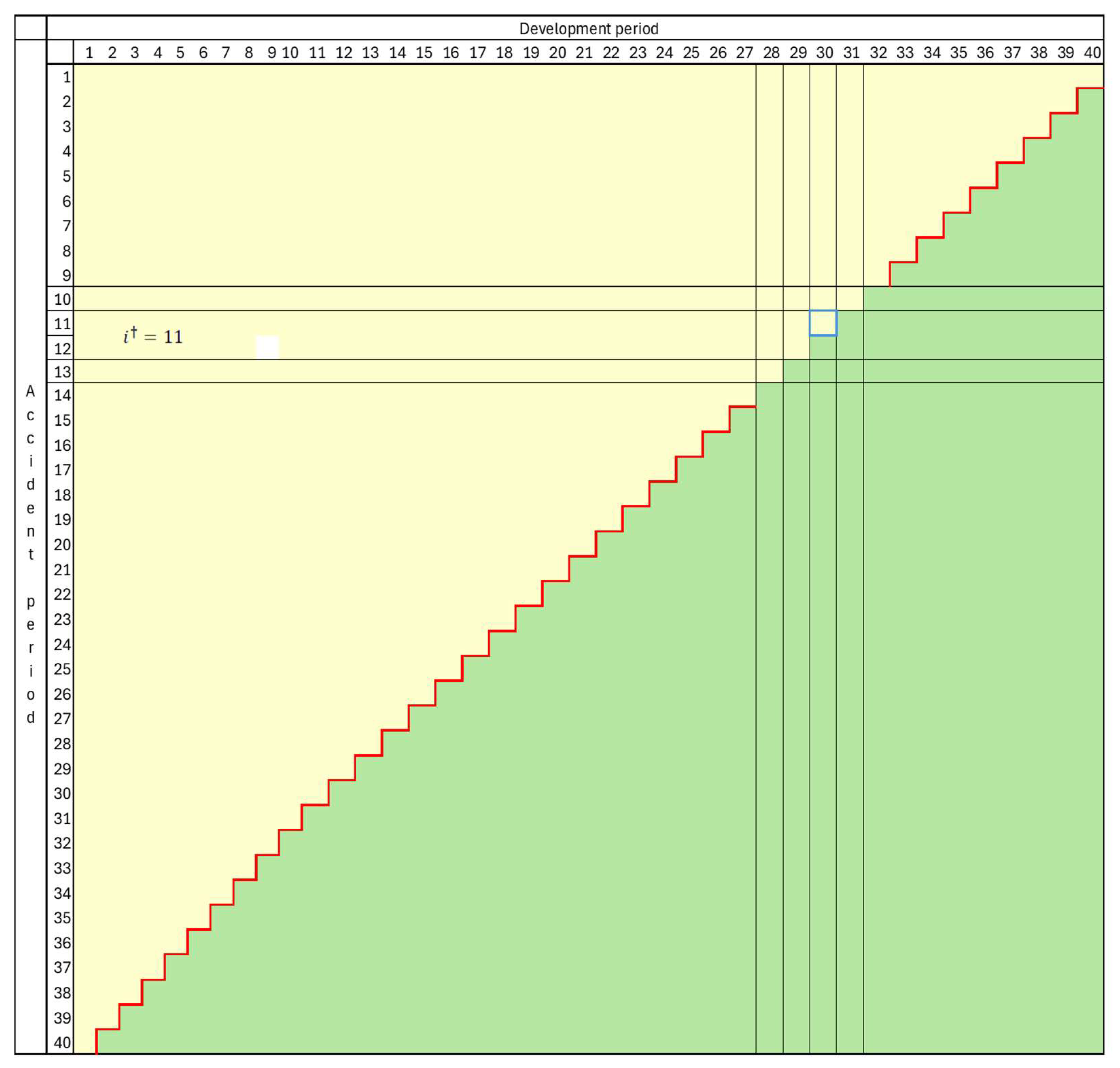
Let the data set consisting of all completed development periods after this merger of accident years be denoted ${\mathcal{D}}_U^{\ast \ast }$. Let ${\mathcal{D}}_L^{\ast \ast }$ denote the corresponding lower triangle, and ${{\mathcal{D}}^{\ast \ast }=\mathcal{D}}_U^{\ast \ast }{\cup \mathcal{D}}_L^{\ast \ast }$. This data set is illustrated in Figure 4 for the case $i^{†}=11$ with accident periods $i^{†},i^{†}+1$ merged.

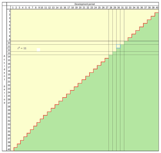
Figure 4. Data set after the merger of accident periods.

Consider the extent to which Assumptions 1 to 6 of Section 3.1 continue to hold in these changed circumstances. The briefest reflection reveals that Assumptions 2, 4 and 5 continue to hold, so attention is now turned to the other assumptions.

• Assumption 1

This assumption evidently holds for all accident periods $i^{\ast }$ other than $i^{†}$, so consider this one. Note that

$$\begin{array}{l}E\left(C_{\left[i^{†}\right]j+1}^{\ast \ast }|C_{i^{†}1},\dots C_{i^{†}j},C_{i^{†}+\mathrm{1,1}},\dots C_{i^{†}+1,j}\right)\\ =E\left(C_{i^{†},j+1}+C_{i^{†}+1,j+1}|C_{i^{†}1},\dots C_{i^{†}j},C_{i^{†}+\mathrm{1,1}},\dots C_{i^{†}+1,j}\right)\\ =C_{\left[i^{†}\right]j}^{\ast \ast }{f}_j.\end{array}$$

where the penultimate equality follows from Assumption 1 in Section 3.1. The only data point on which right side here is $C_{\left[i^{†}\right]j}^{\ast \ast }$, and so it follows that

$$E\left(C_{\left[i^{†}\right]j+1}^{\ast \ast }|C_{\left[i^{†}\right]1}^{\ast \ast },\dots ,C_{\left[i^{†}\right]j}^{\ast \ast }\right)=C_{\left[i^{†}\right]j}^{\ast \ast }{f}_j ,$$

(75)

This shows that Assumption 1 continues to hold in the present circumstances. Note that the age-to-age factors $f_j$ are unchanged by the merger of accident periods.

• Assumption 3

In this case,

$$\begin{gathered} Var\left(C_{\left[i^{†}\right]j+1}^{\ast \ast }|C_{\left[i^{†}\right]0}^{\ast \ast },\dots ,C_{\left[i^{†}\right]j}^{\ast \ast }\right)=Var\left(C_{i^{†},j+1}+C_{i^{†}+1,j+1}|C_{\left[i^{†}\right]0}^{\ast \ast },\dots ,C_{\left[i^{†}\right]j}^{\ast \ast }\right) \\ =Var\left(C_{i^{†},j+1}|C_{\left[i^{†}\right]0}^{\ast \ast },\dots ,C_{\left[i^{†}\right]j}^{\ast \ast }\right) \\ +Var\left(C_{i^{†}+1,j+1}|C_{\left[i^{†}\right]0}^{\ast \ast },\dots ,C_{\left[i^{†}\right]j}^{\ast \ast }\right) , \end{gathered}$$

by Assumption 2. Then, by Assumption 3 and an argument similar to that leading to (75),

$$Var\left(C_{\left[i^{†}\right]j+1}^{\ast \ast }|C_{\left[i^{†}\right]0}^{\ast \ast },\dots ,C_{\left[i^{†}\right]j}^{\ast \ast }\right)=C_{\left[i^{†}\right]j}^{\ast \ast }{\sigma }_j^2 .$$

(76)

This shows that Assumption 3 continues to hold in the present circumstances. Note that the variance factors ${\sigma }_j^2$ are unchanged by the merger of accident periods.

• Assumption 6

In this case, Assumption 6 of Section 3.1 must be modified to the following.

Assumption 6**.

$\sum _{i^{\ast }=1}^{I-j}{c}_{\left[i^{\ast }\right]j}^{\ast \ast }\ne 0,j=1,\dots ,I-1$.

Here, and in the following, the ** notation always indicates quantities relating to ${\mathcal{D}}^{\ast \ast }$.

When Assumptions 1 to 5 and 6** hold, the Mack chain ladder model applies to the data set ${\mathcal{D}}^{\ast \ast }$. It is seen from Figure 4 that a Mack chain ladder model could be imposed on this data set in the usual way, even for the merged accident period, but with the exception of cell (11, 30), or in general cell $\left(i^{†},I-i^{†}+1\right)$. For completeness, the merged cell containing this one must also include $\left(i^{†}+1,I-i^{†}+1\right)$ in order to be usable, but this is as yet unobserved.

Hence, the chain ladder would be imposed on the data set ${\mathcal{D}}_U^{\ast \ast }\backslash \left(i^{†},I-i^{†}+1\right)$, and it would be required that the forecast of the merged accident period be based on the last complete observation $C_{\left[i^{†}\right],I-i^{†}}^{\ast \ast }$. Subject to the exclusion of this single cell, parameter estimation is exactly as for a conventional Mack chain ladder. The same is true for the forecast, except for the merged accident period $\left[i^{†}\right]$. As foreshadowed just above, the forecast of ultimate claim cost in this case is (c.f. (56))

$${\widehat{C}}_{\left[i^{†}\right],I}^{\ast \ast }=c_{\left[i^{†}\right],I-i^{†}}^{\ast \ast }{\widehat{F}}_{I-i^{†}:I}^{\ast \ast } ,$$

(77)

Corresponding to (23) and (57) is

$${\widehat{R}}_{\left[i^{†}\right]}^{\ast \ast }={\widehat{C}}_{\left[i^{†}\right],I}^{\ast \ast }-\left({\mathrm{c}}_{i^{†},I-i^{†}+1}+{\mathrm{c}}_{i^{†}+1,I-i^{†}}\right).$$

(78)

As noted in relation to (57), the value of ${\mathrm{c}}_{i,I-i+1}$ is known for the purpose of (78) though not usable in the estimation of an age-to-age factor.

Lemma 1 now gives the variance of the estimated loss reserve for the combined accident periods $i^{†}$ and $i^{†}+1$. The proof is given in Appendix A.3.

Lemma 1.

The variance $Var\left[{\widehat{R}}_{\left[i^{†}\right]}^{\ast \ast }|{\mathcal{D}}_U^{\ast \ast }\right]$ takes the following form:

$$Var\left[{\widehat{R}}_{\left[i^{†}\right]}^{\ast \ast }|{\mathcal{D}}_U^{\ast \ast }\right]={\left(C_{\left[i^{†}\right]I}^{I-i^{†}}{+C}_{\left[i^{†}+1\right]I}^{I-i^{†}}\right)}^2{V}_{\left[i^{†}\right]}^{I-i^{†}\ast \ast },$$

(79)

where  $V_{\left[i^{†}\right]}^{I-i^{†}\ast \ast }$  is given by

$$V_{\left[i^{†}\right]}^{I-i^{†}\ast \ast }=\sum _{j=I-i^{†}}^{I-1}\left(B_{\left[i^{†}\right],j,I-i^{†}}^{\ast \ast }+{\displaystyle \frac{{\sigma }_j^2}{f_j^2}}{\displaystyle \frac{1}{s_j^{-\ast \ast }}}\right),$$

(80)

$$B_{\left[i^{†}\right],j,I-i^{†}}^{\ast \ast }={\displaystyle \frac{{\sigma }_j^2}{f_j^2}}{\displaystyle \frac{1}{c_{\left[i^{\ast \ast }\right],I-i^{†}}^{\ast \ast }{F}_{I-i^{†}:j}}}={\displaystyle \frac{{\sigma }_j^2}{f_j^2}}{\displaystyle \frac{1}{\left(C_{i^{†},I-i^{†}}+C_{i^{†}+1,I-i^{†}}\right)F_{I-i^{†}:j}}} .$$

(81)

 and

$$\begin{array}{cc}\hfill s_j^{-\ast \ast }& =\sum _{k=1}^{i^{†}-1}{c}_{kj}=s_j^{-}-c_{i^{†}j},j=I-i^{†},\hfill \\ & =s_j^{-},j>I-i^{†}.\hfill \end{array}$$

(82)

Further

$$Var\left[{\widehat{R}}_{i^{†}}+{\widehat{R}}_{i^{†}+1}|{\mathcal{D}}_U\right]=\left(1+2{\zeta }_{i^{†},I-i^{†}}{f}_{I-i^{†}}\right){\left(C_{i^{†}I}^{I-i^{†}+1}\right)}^2{V}_{i^{†}}^{I-i^{†}+1}+{\left(C_{i^{†}+1,I}^{I-i^{†}}\right)}^2{V}_{i^{†}+1}^{I-i^{†}}.$$

(83)

where

$${\zeta }_{i^{†},I-i^{†}}={\displaystyle \frac{c_{i^{†}+1,I-i^{†}}}{c_{i^{†},I-i^{†}+1}}} .$$

(84)

It is now possible to compare $Var\left[{\widehat{R}}_{\left[i^{†}\right]}^{\ast \ast }|{\mathcal{D}}_U^{\ast \ast }\right]$ and $Var\left[{\widehat{R}}_{i^{†}}+{\widehat{R}}_{i^{†}+1}|{\mathcal{D}}_U\right].$ The difference between the variance of estimated loss forecast for merged and unmerged accident periods is now given by

$$\begin{array}{l}Var\left[{\widehat{R}}_{\left[i^{†}\right]}^{\ast \ast }|{\mathcal{D}}_U^{\ast \ast }\right]-Var\left[{\widehat{R}}_{i^{†}}+{\widehat{R}}_{i^{†}+1}|{\mathcal{D}}_U\right]\\ ={\left(C_{\left[i^{†}\right]I}^{I-i^{†}}{+C}_{\left[i^{†}+1\right]I}^{I-i^{†}}\right)}^2{V}_{\left[i^{†}\right]}^{I-i^{†}\ast \ast }\\ -\left[\left(1+2{\zeta }_{i^{†},I-i^{†}}{f}_{I-i^{†}}\right){\left(C_{i^{†}I}^{I-i^{†}+1}\right)}^2{V}_{i^{†}}^{I-i^{†}+1}+{\left(C_{i^{†}+1,I}^{I-i^{†}}\right)}^2{V}_{i^{†}+1}^{I-i^{†}}\right],\end{array}$$

(85)

It is of interest to find characterizations of the positivity and negativity of this difference. Lemma 2 is useful for this purpose. The strategy here is to re-express (85) in such a way that all $C$ terms appearing are the same, and similarly all $V$ terms. Specifically, the only $C$ terms appearing are $C_{i^{†}I}^{I-i^{†}+1}$ and the only $V$ terms are $V_{i^{†}}^{I-i^{†}+1}$. The proof is given in Appendix A.4.

Lemma 2.

For brevity here, $i^{†}$ and ${I-i}^{†}$ are abbreviated to $i$ and $k$. Then the subject of (85) may be expressed as

$$\begin{gathered} Var\left[{\widehat{R}}_{\left[i^{†}\right]}^{\ast \ast }|{\mathcal{D}}_U^{\ast \ast }\right]-Var\left[{\widehat{R}}_{i^{†}}+{\widehat{R}}_{i^{†}+1}|{\mathcal{D}}_U\right]=Var\left[{\widehat{R}}_{\left[i\right]}^{\ast \ast }|{\mathcal{D}}_U^{\ast \ast }\right]-Var\left[{\widehat{R}}_i+{\widehat{R}}_{i+1}|{\mathcal{D}}_U\right] \\ =\{{\gamma }_{ik}^{-2}\left[1+2{\zeta }_{ik}\left({1-\pi }_i^k\right)+{\left(1+{\zeta }_{ik}\right)}^2{\eta }_{ik}{\omega }_{ik}\right][{\omega }_{i,k-1} \\ +{1-\pi }_i^{k+1}+{{\pi }_i^{k+1}\gamma }_{ik}]-\left(1+2{\zeta }_{ik}{f}_k\right)\}{\left(C_{iI}^{k+1}\right)}^2{V}_i^{k+1}. \end{gathered}$$

(86)

where

$${\eta }_{ik}={\left({\displaystyle \frac{s_k^{-}}{c_{ik}}}-1\right)}^{-1}{\displaystyle \frac{\frac{{\sigma }_k^2}{f_k^2}\frac{1}{s_k^{-}}}{B_{ikk}}}>0 .$$

(87)

Proposition 9.

A necessary and sufficient condition that $Var\left[{\widehat{R}}_{\left[i^{†}\right]}^{\ast \ast }|{\mathcal{D}}_U^{\ast \ast }\right]>(=,<)Var\left[{\widehat{R}}_{i^{†}}+{\widehat{R}}_{i^{†}+1}|{\mathcal{D}}_U\right]$ is

$${{\gamma }_{ik}<\left(=,>\right)\tilde{\gamma }}_{ik}^0 ,$$

(88)

where, for brevity, $i,k denote i^{†},I-i^{†}+1$, and ${\tilde{\gamma }}_{i,k-1}^0$ is defined by

$${\tilde{\gamma }}_{ik}^0=½{\tilde{\pi }}_i^{k+1}+{\left|1-½{\tilde{\pi }}_i^{k+1}\right|\left(1+{\displaystyle \frac{{\tilde{\omega }}_{ik}+\left({\xi }_{ik}-1\right)}{{\left(1-½\left({\tilde{\pi }}_i^{k+1}\right)\right)}^2}}\right)}^{½},$$

(89)

where

$${\xi }_{ik}={\left(1+2{\zeta }_{ik}{f}_k\right)}^{-1}\left[1+2{\zeta }_{ik}\left({1-\pi }_i^k\right)+{\left(1+{\zeta }_{ik}\right)}^2{\eta }_{ik}{\omega }_{ik}\right],$$

(90)

$${\tilde{\pi }}_i^{k+1}={\xi }_{ik}{\pi }_i^{k+1},$$

(91)

$${\tilde{\omega }}_{ik}={\xi }_{ik}{\omega }_{ik} .$$

(92)

Note the similarity between (69) and (89). After the conversion of quantities to tilda versions, the two results are almost identical.

A fairly weak condition is required to establish that ${\gamma }_{ik}^0\ge 1/{\xi }_{ik}$, as testified by Corollary 2, which is proved in Appendix A.6.

Corollary 2.

A sufficient condition that ${\gamma }_{ik}^0\ge 1/{\xi }_{ik}$ is that

$$\left(1+{\omega }_{ik}\right)\left(1-{\pi }_i^k\right)\le f_k.$$

(93)

Note that, as ${\xi }_{ik}$ increases, the lower bound on the critical value ${\gamma }_{ik}^0$ becomes steadily smaller. For large values of ${\xi }_{ik}$, the bound approaches zero. This means that only very small values of ${\gamma }_{ik}$ are shown to guarantee that increased granularity reduces the variance of the predicted loss reserve. This result stands in stark relief against that of Corollary 1 in the case of an increased granularity within a single accident period.

The physical meaning of large or small values of ${\xi }_{ik}$ is not clear, but it is a function of ${\zeta }_{ik}$ that does have a clear meaning (see (84)). There is therefore value in examining the relation between ${\zeta }_{ik}$ and ${\xi }_{ik}$. Table 4 does so, examining three key values of ${\zeta }_{ik}$.

Table 4. Relation between ${\mathit{\zeta }}_{\mathit{i}\mathit{k}}$ and ${\mathit{\xi }}_{\mathit{i}\mathit{k}}.$

$\mathbf{Value} \mathbf{of} {\mathit{\zeta }}_{\mathit{i}\mathit{k}}$	$\mathbf{Value} \mathbf{of} {\mathit{\xi }}_{\mathit{i}\mathit{k}}$
0	$1+{\eta }_{ik}{\omega }_{ik}$
1	${\left(1+2f_k\right)}^{-1}\left[3-2{\pi }_i^k+4{\eta }_{ik}{\omega }_{ik}\right]$
$\infty$	$\infty$

For an intuition for these values, recall from (64) that ${0<\pi }_i^k<1$ and from (70) and (87) that, in many applications, ${\omega }_{ik}$ and ${\omega }_{ik}$ will be small relative to unity.

By (84), ${\zeta }_{ik}$ measures the volume of claims in the accident period $i+1$ relative to that in $i$. Combining Corollary 2 with Table 4 gives an indication of how variation of ${\zeta }_{ik}$ changes the effect of granularity on the variance of forecast loss reserve. For example, if accident period $i+1$ heavily dominates $i$ (${\zeta }_{ik}\to \infty$), then ${\xi }_{ik}$ is large, and Corollary 2 indicates that the separation of the two accident periods is unlikely to be of benefit to the variance. This is consistent with intuition.

As a further example, suppose that ${\zeta }_{ik}=1$, implying equal claim volumes in accident periods $i+1$ and $i$. Suppose also that ${\pi }_i^k=½$ and $f_k=1.2$. Then, by Table 4, ${\xi }_{ik}$ will be somewhat greater than 0.59. Then, if condition (93) is satisfied, Corollary 2 reveals that ${\gamma }_{ik}^0$ is somewhat less than 1.7.

If the conclusion of Corollary 2 is a relatively tight inequality, then there is considerable benefit in the increased granularity of maintaining the separation of accident periods $i+1$ and $i$.

The reasons why a decrease in granularity does not always lead to an enlargement of the variance of forecast loss reserve are apparent from (79) and (83).

In the former of these relations, it is seen that the merger of the two accident periods causes both to be forecasts as at time $I-i^{†}$ (instead of $I-i^{†}+1$ in one case), resulting in a loss of information. This is exactly what happened in the merger of development periods in Section 4.2.1.

On the other hand, however, relation (83) shows that, when the separation of accident periods is maintained, positive covariance arises between their forecasts of loss reserve. This is the term involving ${\zeta }_{ik}$, and it increases the variance of loss reserve of the aggregated accident periods.

Whether or not increased granularity is beneficial depends on the net effect of these opposing forces.

Remark 3.

The above analysis has considered only the merger of accident periods $i^{†}$ and $i^{†}+1$ . However, the analysis can be repeated for further mergers. Suppose, for example, that the original development periods were months and one wished to form quarterly periods, perhaps involving the merger of $i^{†},i^{†}+1$ and $i^{†}+2$. One could commence with the merger of periods $i^{†}$ and $i^{†}+1$, as just analyzed.

One could then merge period $i^{†}+2$ with the combination of the first two. The above analysis would then apply equally to this merger of two accident periods. Two-period mergers could be continued in this way until the desired final set of merged accident periods was attained. The conclusions would be as above, specifically that

• The reduction in granularity increases the variance of estimated loss reserve unless (88) holds with the relation >;
• At each merger, the thresholds ${\gamma }_{i^{†},k-1}^0$ appearing in (88) can be calculated and the likelihood of that relation assessed.

5. Discussion and Conclusions

Taylor (2025) showed that, when the EDF chain ladder is applied to a data triangle, greater data granularity always reduces the variance of the estimated loss reserve. The present paper considers a parallel question in relation to the Mack chain ladder, an alternative model form.

As in Taylor (2025), two types of increases in the mesh size of the data triangle are introduced:

• Preserving calendar periods;
• Preserving development periods;

but considerations of space limit the present paper to just the latter (Section 4). The former type of change of mesh may be considered in a separate paper.

The first question requiring consideration concerns whether the assumptions underpinning the Mack chain ladder in relation to the original data set continue to hold when specific development periods are merged. Proposition 4 finds that they do so under some mild regularity conditions.

Section 4.2 studies the changes in variance of the estimated loss reserve when the mesh size is changed, first when development periods are merged (Section 4.2.1) and then when accident periods are merged (Section 4.2.2). The consideration of changes in both of these dimensions is necessary as one may wish to compare the situations in, say, a $40\times 40$ triangle that uses quarterly units of time and its derivative $10\times 10$ triangle.

Section 4.2.1 considers the case in which just two consecutive development periods are merged, but all other development periods and all accident periods are left unchanged.

Here, results similar, but not identical, to those in Taylor (2025) are found. The variances of loss reserves are unchanged except in the case of a single specific accident period.

It is no longer the case that greater data granularity is guaranteed to reduce the variance of the estimated loss reserve. Whether or not a reduction occurs depends on the data points observed. The reason for this difference is essentially that, in the case of the Mack model, the standard deviation of the estimated loss reserve with respect to a particular accident period is proportional to the cumulative claim payments to date, whereas this is not so for the EDF chain ladder.

A reduction in variance does in fact occur if a defined condition on the data of the specific accident period subject to change is satisfied. The condition is that the ratio of the last observed age-to-age factor for the accident period to its expected value falls below a threshold whose value is defined in Proposition 8. It takes the form of a closed-form function of the data and the chain ladder parameters (age-to-age factors).

It is noteworthy that this threshold value always exceeds unity. Hence, an observed value of the ratio in question below unity is sufficient to indicate a reduction in the variance of the loss reserve estimate (Corollary 1). When the ratio exceeds unity, the occurrence or otherwise of variance depends on the threshold value, which is a matter of numerical evaluation.

A numerical example is given in Section 4.2.1, where it is found that the condition for variance reduction is comfortably satisfied for each possible merger of two consecutive development periods. There is plenty of scope for further numerical investigation, but the ease with which the necessary condition is met in this one example prompts a conjecture that counter-examples might sometimes require a certain degree of contrivance and that greater granularity would frequently, if not usually, lead to a reduction in variance of estimated loss reserve in practical cases.

All of these results hitherto have concerned the simple case in which two consecutive development periods are merged. However, Remark 2 points out that it is a simple matter to extrapolate to parallel results for an arbitrary merger of development periods.

Section 4.2.2 considers the merger of accident periods. Again, the Mack chain ladder remains valid under mild regularity conditions. It is found that the conditions for a reduction in variance of estimated loss reserve in this case are much more complex than in Section 4.2.1 for the merger of development periods.

As in Section 4.2.1, a reduction in variance with increased granularity is guaranteed if the ratio of the last observed age-to-age factor for the accident period to its expected value falls below a threshold. The threshold value is defined in Proposition 9 and, once again, it takes the form of a closed form function of the data and the chain ladder parameters.

In this case, however, the function is much more complex and less transparent than in Section 4.2.1. Moreover, as pointed out in Corollary 2, it produces a much stricter condition on the chain ladder parameters if variance reduction is to be guaranteed.

This point is discussed in Section 4.2.2, where the reason is identified as the correlation between the forecast loss reserves associated with distinct and unmerged accident periods. Whether variance reduction is achieved depends heavily on the relative volumes of claims in the respective accident periods subject to merger.

Although the threshold values mentioned above are readily available numerically, specific analytic results appear hard to come by in this area. Section 4.2.2 contains some indicative numerical clues.

All in all, the influence of data granularity on the variance of forecast loss reserve differs vastly between the EDF chain ladder and the Mack chain ladder. This seems remarkable for two models that produce precisely the same forecasts using precisely the same estimation algorithm.

Appendix A.1

Proof of Proposition 2.

Equation (34) yields the following at evaluation point $k-1$:

$$V_i^{k-1}=\sum _{j=k-1}^{I-1}\left(B_{ij,k-1}++{\displaystyle \frac{{\sigma }_j^2}{f_j^2}}{\displaystyle \frac{1}{s_j^{-}}}\right)=\left(B_{i,k-1,k-1}++{\displaystyle \frac{{\sigma }_{k-1}^2}{f_{k-1}^2}}{\displaystyle \frac{1}{s_{k-1}^{-}}}\right)+\sum _{j=k}^{I-1}\left(B_{ij,k-1}+{\displaystyle \frac{{\sigma }_j^2}{f_j^2}}{\displaystyle \frac{1}{s_j^{-}}}\right).$$

(A1)

Now,

$$B_{ij,k-1}={\displaystyle \frac{{\sigma }_j^2}{f_j^2}}{\displaystyle \frac{1}{c_{i,k-1}{F}_{k-1:j}}}={\displaystyle \frac{{\sigma }_j^2}{f_j^2}}{\displaystyle \frac{c_{ik}}{c_{i,k-1}{f}_{k-1}}} {\displaystyle \frac{1}{c_{ik}{F}_{k:j}}}={\displaystyle \frac{c_{ik}}{c_{i,k-1}{f}_{k-1}}} B_{ijk} .$$

(A2)

The substitution of (A2) into (A1) yields

$$\begin{gathered} V_i^{k-1}=\left(B_{i,k-1,k-1}+{\displaystyle \frac{{\sigma }_{k-1}^2}{f_{k-1}^2}}{\displaystyle \frac{1}{s_{k-1}^{-}}}\right)+\left(1-{\displaystyle \frac{c_{ik}}{c_{i,k-1}{f}_{k-1}}}\right)\sum _{j=k}^{I-1}{\displaystyle \frac{{\sigma }_j^2}{f_j^2}}{\displaystyle \frac{1}{s_j^{-}}} \\ +{\displaystyle \frac{c_{ik}}{c_{i,k-1}{f}_{k-1}}}\sum _{j=k}^{I-1}\left(B_{ijk}+{\displaystyle \frac{{\sigma }_j^2}{f_j^2}}{\displaystyle \frac{1}{s_j^{-}}}\right), \end{gathered}$$

(A3)

and the proposition follows. □

Appendix A.2

Proof of Proposition 8.

The substitution of (21) into the quantity on the right side of (63) yields

$$\begin{array}{l}{\left(C_{I-j^{†}+1,I}^{j^{†}-1}\right)}^2{V}_{I-j^{†}+1}^{j^{†}-1}-{\left(C_{I-j^{†}+1:I}^{j^{†}}\right)}^2{V}_{I-j^{†}+1}^{j^{†}}\\ ={\left(c_{I-j^{†}+1,j^{†}-1}{F}_{j^{†}-1:I}\right)}^2{V}_{I-j^{†}+1}^{j^{†}-1}-{\left(c_{I-j^{†}+1,j^{†}}{F}_{j^{†}:I}\right)}^2{V}_{I-j^{†}+1}^{j^{†}} .\end{array}$$

(A4)

For brevity, it will be convenient to temporarily replace (just for the present proof) $I-j^{†}+1$ by $i$ and $j^{†}$ by $k$, whereupon (A4) becomes

$$\begin{array}{l}{\left(C_{I-j^{†}+1,I}^{j^{†}-1}\right)}^2{V}_{I-j^{†}+1}^{j^{†}-1}-{\left(C_{I-j^{†}+1:I}^{j^{†}}\right)}^2{V}_{I-j^{†}+1}^{j^{†}}\\ ={\left(c_{i,k-1}{F}_{k-1:I}\right)}^2\left[V_i^{k-1}-{\left({\displaystyle \frac{c_{ik}}{c_{i,k-1}{f}_{k-1}}}\right)}^2{V}_i^k\right]\\ ={\left(c_{i,k-1}{F}_{k-1:I}\right)}^2\left[V_i^{k-1}-{\gamma }_{i,k-1}^2{V}_i^k\right],\end{array}$$

(A5)

where use has been made of (27) and (37).

Now substitute (36) for $V_i^{k-1}$ to obtain

$$\begin{array}{l}{V}_i^{k-1}-{\gamma }_{i,k-1}^2{V}_i^k=\left[\left(B_{i,k-1,k-1}+{\displaystyle \frac{{\sigma }_{k-1}^2}{f_{k-1}^2}}{\displaystyle \frac{1}{s_{k-1}^{-}}}\right)+\sum _{j=k}^{I-1}{\displaystyle \frac{{\sigma }_j^2}{f_j^2}}{\displaystyle \frac{1}{s_j^{-}}}\right]\\ +{\gamma }_{i,k-1}\left(V_i^k-\sum _{j=k}^{I-1}{\displaystyle \frac{{\sigma }_j^2}{f_j^2}}{\displaystyle \frac{1}{s_j^{-}}}\right)-{\gamma }_{i,k-1}^2{V}_i^k .\end{array}$$

(A6)

Substitute (66) into (A6), divide through by $V_i^k$, and then substitute (64) into the result to obtain

$${\displaystyle \frac{V_i^{k-1}-{\gamma }_{i,k-1}^2{V}_i^k}{V_i^k}}=\left[\left(1-{\pi }_i^k\right)+{\omega }_{i,k-1}\right]+{{\pi }_i^k\gamma }_{i,k-1}-{\gamma }_{i,k-1}^2 ,$$

(A7)

where ${\omega }_{i,k-1}$ is defined by (70).

The right side is merely a quadratic in ${\gamma }_{i,k-1}$, and its zeros are

$$\begin{array}{l}{\gamma }_{i,k-1}={½\pi }_i^k\mp ½{\left({\left({\pi }_i^k\right)}^2+4\left(\left(1-{\pi }_i^k\right)+{\omega }_{i,k-1}\right)\right)}^{½}\\ ={½\pi }_i^k\mp {\left(1-½{\pi }_i^k\right)\left(1+{\displaystyle \frac{{\omega }_{i,k-1}}{{\left(1-½{\pi }_i^k\right)}^2}}\right)}^{½}.\end{array}$$

(A8)

Note that, since the square root here is strictly positive, one of these zeros is $>1$, and the other is $<{\pi }_i^k-1$. It was shown in (67) that ${\pi }_i^k<1$, and so this second zero is strictly negative. This zero is meaningless as ${\gamma }_{i,k-1}$ cannot be negative. The first zero is meaningful and will be denoted by ${\gamma }_{i,k-1}^0\left(>1\right)$.

It is evident from the signs of the coefficients in (A7) that the quadratic changes from positive to negative at ${{\gamma }_{i,k-1}=\gamma }_{i,k-1}^0$, and so $V_i^{k-1}-{\gamma }_{i,k-1}^2{V}_i^k>\left(<\right)0$ according to ${{\gamma }_{i,k-1}<\left(>\right)\gamma }_{i,k-1}^0$. The required result is then obtained by restoring $i,k$ to their original values, $I-j^{†}+1,j^{†}$. □

Appendix A.3

Proof of Lemma 1.

As seen in the preamble to the lemma, when the available data set is ${\mathcal{D}}_U^{\ast \ast }$, the chain ladder model is applied to ${\mathcal{D}}_U^{\ast \ast }\backslash \left(i^{†},I-i^{†}+1\right)$, and expected age-to-age and variance factors are unchanged relative to the model applied to ${\mathcal{D}}_U$:

$$f_j^{\ast \ast }=f_j,{\sigma }_j^{2\ast \ast }={\sigma }_j^2.$$

(A9)

Moreover,

$$\begin{gathered} C_{\left[i^{\ast \ast }\right]j}^{\ast \ast }=C_{i^{\ast \ast },j}+C_{i^{\ast \ast }+1,j},i^{\ast \ast }=i^{†}; \\ =C_{i^{\ast \ast },j},i^{\ast \ast }<i^{†} \\ =C_{i^{\ast \ast }+1,j},i^{\ast \ast }>i^{†} . \end{gathered}$$

(A10)

The quantity $Var\left[{\widehat{R}}_{\left[i^{†}\right]}^{\ast \ast }|{\mathcal{D}}_U^{\ast \ast }\right]$ is represented by (32) to (35), adapted to the new data set ${\mathcal{D}}_U^{\ast \ast }$, specifically,

$$Var\left[{\widehat{R}}_{\left[i^{†}\right]}^{\ast \ast }|{\mathcal{D}}_U^{\ast \ast }\right]=Var\left[{\widehat{R}}_{\left[i^{†}\right]}^{I-i^{†}\ast \ast }|{\mathcal{D}}_U^{\ast \ast }\right]={\left(C_{\left[i^{†}\right]I}^{I-i^{†}\ast \ast }\right)}^2{V}_{\left[i^{†}\right]}^{I-i^{†}\ast \ast }={\left(C_{\left[i^{†}\right]I}^{I-i^{†}}{+C}_{\left[i^{†}+1\right]I}^{I-i^{†}}\right)}^2{V}_{\left[i^{†}\right]}^{I-i^{†}\ast \ast },$$

(A11)

where $V_{\left[i^{†}\right]}^{I-i^{†}\ast \ast }$ is given by (80) to (82).

To prove (83), note that

$$\begin{array}{l}Var\left[{\widehat{R}}_{i^{†}}+{\widehat{R}}_{i^{†}+1}|{\mathcal{D}}_U\right]\\ =Var\left[{\widehat{R}}_{i^{†}}^{I-i^{†}+1}|{\mathcal{D}}_U\right]+\mathrm{V}\mathrm{a}\mathrm{r}\left[{\widehat{R}}_{i^{†}+1}^{I-i^{†}}|{\mathcal{D}}_U\right]\\ +2\mathrm{C}\mathrm{o}\mathrm{v}\left[{\widehat{R}}_{i^{†}}^{I-i^{†}+1},{\widehat{R}}_{i^{†}+1}^{I-i^{†}}|{\mathcal{D}}_U\right].\end{array}$$

(A12)

For brevity, in the following, $i$ and $k$ will be used to denote $i^{†}$ and ${I-i}^{†}$ , respectively. By (29),

$$\mathrm{V}\mathrm{a}\mathrm{r}\left[{\widehat{R}}_{i+r}^{k+1-r}|{\mathcal{D}}_U\right]={\left(C_{i+r,I}^{k+1-r}\right)}^2{V}_{i+r}^{k+1-r},r=\mathrm{0,1}.$$

(A13)

Now

$${\widehat{R}}_{i+r}^{k+1-r}=c_{i+r,k+1-r}{\widehat{F}}_{k+1-r:I}-c_{i+r,k+1-r},\mathrm{r}=\mathrm{0,1},$$

(A14)

and so

$$\mathrm{C}\mathrm{o}\mathrm{v}\left[{\widehat{R}}_i^{k+1},{\widehat{R}}_{i+1}^k|{\mathcal{D}}_U\right]=c_{i,k+1}{c}_{i+1,k}\mathrm{C}\mathrm{o}\mathrm{v}\left[{\widehat{F}}_{k:I}{,\widehat{F}}_{k+1:I}\right]=c_{i,k+1}{c}_{i+1,k}{f}_k{\left({\displaystyle \frac{C_{iI}^{k+1}}{c_{i,k+1}}}\right)}^2{V}_i^{k+1},$$

(A15)

where the final expression follows from (42).

Substitution of (84) into (A15) reduces the latter to

$$\mathrm{C}\mathrm{o}\mathrm{v}\left[{\widehat{R}}_i^{k+1},{\widehat{R}}_{i+1}^k|{\mathcal{D}}_U\right]={\zeta }_{ik}{f}_k{\left(C_{iI}^{k+1}\right)}^2{V}_i^k.$$

(A16)

Finally, the substitution of (A13) and (A16) into (A12) yields the stated result of the lemma after the translation of $i,k$ back to their original meanings. □

Appendix A.4

Proof of Lemma 2.

The translation of (85) into the “$i,k$ notation” introduced in the lemma is

$$\begin{array}{l}Var\left[{\widehat{R}}_{\left[i^{†}\right]}^{\ast \ast }|{\mathcal{D}}_U^{\ast \ast }\right]-Var\left[{\widehat{R}}_{i^{†}}+{\widehat{R}}_{i^{†}+1}|{\mathcal{D}}_U\right]\\ ={\left(C_{iI}^k{+C}_{i+1,I}^k\right)}^2{V}_i^{k\ast \ast }\\ -\left[\left(1+2{\zeta }_{ik}{f}_k\right){\left(C_{iI}^{k+1}\right)}^2{V}_i^{k+1}+{\left(C_{i+1,I}^k\right)}^2{V}_{i+1}^k\right].\end{array}$$

(A17)

As mentioned in the preamble to the lemma, all $C$ and $V$ terms are adjusted so that only $C_{iI}^{k+1}$ and $V_i^{k+1}$ appear.

C terms

By (31) and (37),

$$C_{iI}^k={\displaystyle \frac{c_{ik}{F}_{k:I}}{c_{i,k+1}{F}_{k+1:I}}}{C}_{iI}^{k+1}={\displaystyle \frac{c_{ik}{f}_k}{c_{i,k+1}}}{C}_{iI}^{k+1}={\gamma }_{ik}^{-1}{C}_{iI}^{k+1}.$$

(A18)

By (31), (84) and (A18),

$$C_{i+1,I}^k={\displaystyle \frac{c_{i+1,k}{F}_{k:I}}{c_{ik}{F}_{k:I}}}{C}_{iI}^k={\zeta }_{ik}{\gamma }_{ik}^{-1}{C}_{iI}^{k+1}.$$

(A19)

V terms

Consider the term $V_i^{k\ast \ast }$, defined by (80) to (82). By (35), (81), and (84),

$$B_{\left[i\right]jk}^{\ast \ast }={{\displaystyle \frac{C_{ik}}{C_{ik}+C_{i+1,k}}}B}_{ijk}={\left(1+{\zeta }_{ik}\right)}^{-1}{B}_{ijk} .$$

(A20)

Further, by comparison of (82) with (4),

$$\sum _{j=k}^{I-1}{\displaystyle \frac{{\sigma }_j^2}{f_j^2}}{\displaystyle \frac{1}{s_j^{-\ast \ast }}}=\sum _{j=k}^{I-1}{\displaystyle \frac{{\sigma }_j^2}{f_j^2}}{\displaystyle \frac{1}{s_j^{-}}}+\left({\displaystyle \frac{{\sigma }_k^2}{f_k^2}}{\displaystyle \frac{1}{s_k^{-}}}\right){\displaystyle \frac{c_{ik}}{s_k^{-\ast \ast }}}=\left(1-{\pi }_i^k+{\eta }_{ik}{\omega }_{ik}\right)V_i^k ,$$

(A21)

where ${\pi }_i^k,{\eta }_{ik},{\omega }_{ik},$ are defined by (64), (70), and (87), respectively.

By (A20) and (A21),

$$V_i^{k\ast \ast }=\left[{\left(1+{\zeta }_{ik}\right)}^{-1}{\pi }_i^k+1-{\pi }_i^k+{\eta }_{ik}{\omega }_{ik}\right]V_i^k .$$

(A22)

The term of (A17) involving $V_{i+1}^k$ can be dealt with similarly by the decomposition of $V_{i+1}^k$ and separate treatment of its two components.

$$V_{i+1}^k=\sum _{j=k}^{I-1}\left(B_{i+1,jk}+{\displaystyle \frac{{\sigma }_j^2}{f_j^2}}{\displaystyle \frac{1}{s_j^{-}}}\right),$$

(A23)

where

$$B_{i+1,jk}={\displaystyle \frac{{\sigma }_j^2}{f_j^2}}{\displaystyle \frac{1}{c_{i+1,k}{F}_{k:j}}}={\zeta }_{ik}^{-1}{\displaystyle \frac{{\sigma }_j^2}{f_j^2}}{\displaystyle \frac{1}{c_{ik}{F}_{k:j}}}={\zeta }_{ik}^{-1}{B}_{ijk},$$

(A24)

and substitution of this in (A23) yields

$$V_{i+1}^k=\left({\zeta }_{ik}^{-1}{\pi }_i^k+1-{\pi }_i^k\right)V_i^k .$$

(A25)

Now re-express (A22) and (A25) in terms of $V_i^{k+1}$. This can be achieved by re-writing (36) in the form

$$\begin{array}{l}{V}_i^k=\left({\omega }_{ik}+\left(1-{\gamma }_{ik}\right)\left({1-\pi }_i^{k+1}\right)+{\gamma }_{ik}\right)V_i^{k+1}\\ =\left({\omega }_{i,k-1}+{1-\pi }_i^{k+1}+{{\pi }_i^{k+1}\gamma }_{ik}\right)V_i^{k+1}.\end{array}$$

(A26)

This converts (A22) and (A25) to the following forms:

$$V_i^{k\ast \ast }=\left[{\left(1+{\zeta }_{ik}\right)}^{-1}{\pi }_i^k+1-{\pi }_i^k+{\eta }_{ik}{\omega }_{ik}\right]\left({\omega }_{ik}+{1-\pi }_i^{k+1}+{{\pi }_i^{k+1}\gamma }_{ik}\right)V_i^{k+1} ,$$

(A27)

$$V_{i+1}^k=\left({\zeta }_{ik}^{-1}{\pi }_i^k+1-{\pi }_i^k\right)\left({\omega }_{ik}+{1-\pi }_i^{k+1}+{{\pi }_i^{k+1}\gamma }_{ik}\right)V_i^{k+1} .$$

(A28)

The three members on the right side of (A17) can now be compiled one by one. By (A18), (A19) and (A27),

$$\begin{array}{l}{\left(C_{iI}^k{+C}_{i+1,I}^k\right)}^2{V}_i^{k\ast \ast }={\gamma }_{ik}^{-2}{\left(1+{\zeta }_{ik}\right)}^2\left[{\left(1+{\zeta }_{ik}\right)}^{-1}{\pi }_i^k+1-{\pi }_i^k+{\eta }_{ik}{\omega }_{ik}\right]({\omega }_{ik}\\ +{1-\pi }_i^{k+1}+{{\pi }_i^{k+1}\gamma }_{ik}){\left(C_{iI}^{k+1}\right)}^2{V}_i^{k+1}.\end{array}$$

(A29)

By (A19) and (A28),

$$\begin{gathered} {\left(C_{i+1,I}^k\right)}^2{V}_{i+1}^k={\gamma }_{ik}^{-2}{\zeta }_{ik}^2\left({\zeta }_{ik}^{-1}{\pi }_i^k+1-{\pi }_i^k\right)({\omega }_{ik}+{1-\pi }_i^{k+1} \\ +{{\pi }_i^{k+1}\gamma }_{ik}){\left(C_{iI}^{k+1}\right)}^2{V}_i^{k+1}. \end{gathered}$$

(A30)

The difference between these two quantities is

$$\begin{array}{l}{\left(C_{iI}^k{+C}_{i+1,I}^k\right)}^2{V}_i^{k\ast \ast }-{\left(C_{i+1,I}^k\right)}^2{V}_{i+1}^k\\ ={\gamma }_{ik}^{-2}\left[{\pi }_i^k+\left(1+2{\zeta }_{ik}\right)\left({1-\pi }_i^k\right)+{\left(1+{\zeta }_{ik}\right)}^2{\eta }_{ik}{\omega }_{ik}\right]({\omega }_{ik}\\ +{1-\pi }_i^{k+1}+{{\pi }_i^{k+1}\gamma }_{ik}){\left(C_{iI}^{k+1}\right)}^2{V}_i^{k+1}.\end{array}$$

(A31)

Finally, including the remaining member from the right side of (A17) yields

$$\begin{array}{l}Var\left[{\widehat{R}}_{\left[i^{†}\right]}^{\ast \ast }|{\mathcal{D}}_U^{\ast \ast }\right]-Var\left[{\widehat{R}}_{i^{†}}+{\widehat{R}}_{i^{†}+1}|{\mathcal{D}}_U\right]\\ =\left\{{\gamma }_{ik}^{-2}\left[1+2{\zeta }_{ik}\left({1-\pi }_i^k\right)+{\left(1+{\zeta }_{ik}\right)}^2{\eta }_{ik}{\omega }_{ik}\right]\right[{\omega }_{ik}+\left({1-\pi }_i^{k+1}\right)\\ +{{\pi }_i^{k+1}\gamma }_{ik}]-\left(1+2{\zeta }_{ik}{f}_k\right)\}{\left(C_{iI}^{k+1}\right)}^2{V}_i^{k+1}.\end{array}$$

(A32)

□

Appendix A.5

Proof of Proposition 9.

The establishment of the necessary and sufficient condition stated in the proposition requires the evaluation of the zeros of the quantity (86) in Lemma 2, as a function of ${\gamma }_{ik}$ , or, equivalently, the quantity

$$\begin{array}{l}Q=\left[1+2{\zeta }_{ik}\left({1-\pi }_i^k\right)+{\left(1+{\zeta }_{ik}\right)}^2{\eta }_{ik}{\omega }_{ik}\right]\left[{\omega }_{ik}+\left({1-\pi }_i^{k+1}\right)+{{\pi }_i^{k+1}\gamma }_{ik}\right]\\ -\left(1+2{\zeta }_{ik}{f}_k\right){\gamma }_{ik}^2.\end{array}$$

(A33)

This is a quadratic in ${\gamma }_{ik}$, so coefficients of different powers of this variable are collected, with the following result.

$$\begin{array}{l}-Q=\left(1+2{\zeta }_{ik}{f}_k\right){\gamma }_{ik}^2-\left[1+2{\zeta }_{ik}\left({1-\pi }_i^k\right)+{\left(1+{\zeta }_{ik}\right)}^2{\eta }_{ik}{\omega }_{ik}\right]{{\pi }_i^{k+1}\gamma }_{ik}\\ -\left[1+2{\zeta }_{ik}\left({1-\pi }_i^k\right)+{\left(1+{\zeta }_{ik}\right)}^2{\eta }_{ik}{\omega }_{ik}\right]\left[{\omega }_{ik}+\left({1-\pi }_i^{k+1}\right)\right],\end{array}$$

(A34)

This may be abbreviated to

$$-{\left(1+2{\zeta }_{ik}{f}_k\right)}^{-1}Q={\gamma }_{ik}^2-{\xi }_{ik}{{\pi }_i^{k+1}\gamma }_{ik}-{\xi }_{ik}\left[{\omega }_{ik}+\left({1-\pi }_i^{k+1}\right)\right]$$

(A35)

where ${\xi }_{ik}$ is defined by (90).

The zeros of this quadratic are obtained by the same process as in (A8), with modification for multiplier ${\xi }_{ik}$. Note the negative sign of the constant term in (A35), which implies one positive and one negative zero. Only the positive zero is of interest. This completes the proof of the proposition. □

Appendix A.6

Proof of Corollary 2.

The condition to be proved is equivalent to ${\tilde{\gamma }}_{ik}^0\ge 1$.

By (89),

$${\tilde{\gamma }}_{ik}^0=½{\tilde{\pi }}_i^{k+1}+\left|1-½{\tilde{\pi }}_i^{k+1}\right|\left(1+X\right),$$

(A36)

where ${\tilde{\omega }}_{ik}+\left({\xi }_{ik}-1\right)$ is a sufficient condition for $X>0$.

There are two cases to be considered.

Case I:  ${\tilde{\mathit{\pi }}}_{\mathit{i}}^{\mathit{k}+\mathbf{1}}\le \mathbf{2}$. In this case,

$${\tilde{\gamma }}_{ik}^0=1+\left(1-½{\tilde{\pi }}_i^{k+1}\right)X\ge 1.$$

(A37)

Case II:  ${\tilde{\mathit{\pi }}}_{\mathit{i}}^{\mathit{k}+\mathbf{1}}>\mathbf{2}$. In this case, (89) becomes

$${\tilde{\gamma }}_{ik}^0=½{\tilde{\pi }}_i^{k+1}+\left(½{\tilde{\pi }}_i^{k+1-1}\right)\left(1+X\right)=\left({\tilde{\pi }}_i^{k+1}-1\right)+\left(½{\tilde{\pi }}_i^{k+1-1}\right)X>1$$

(A38)

Thus, ${\tilde{\omega }}_{ik}+\left({\xi }_{ik}-1\right)>0$ is a sufficient condition for ${\tilde{\gamma }}_{ik}^0\ge 1$ in general.

Therefore, the remainder of this proof will address the requirement that ${\tilde{\omega }}_{ik}+\left({\xi }_{ik}-1\right)>0$. The quantity on the left side of this inequality may be expressed as

$$\begin{array}{l}{\tilde{\omega }}_{ik}+\left({\xi }_{ik}-1\right)={\xi }_{ik}\left(1+{\omega }_{ik}\right)-1\\ ={\left(1+2{\zeta }_{ik}{f}_k\right)}^{-1}\left\{\left(1+{\omega }_{ik}\right)\right[1+2{\zeta }_{ik}\left({1-\pi }_i^k\right)\\ +{\left(1+{\zeta }_{ik}\right)}^2{\eta }_{ik}{\omega }_{ik}]-\left(1+2{\zeta }_{ik}{f}_k\right)\}\\ ={\left(1+2{\zeta }_{ik}{f}_k\right)}^{-1}\{{\eta }_{ik}{\omega }_{ik}\left(1+{\omega }_{ik}\right){\zeta }_{ik}^2\\ +2{\zeta }_{ik}\left[\left(1+{\omega }_{ik}\right)\left({1-\pi }_i^k+{\eta }_{ik}{\omega }_{ik}\right)-f_k\right]\\ +{\omega }_{ik}\left[1+{\eta }_{ik}\left(1+{\omega }_{ik}\right)\right]\}.\end{array}$$

(A39)

Thus

$$\begin{array}{l}\left(1+2{\zeta }_{ik}{f}_k\right){\left({\eta }_{ik}{\omega }_{ik}\left(1+{\omega }_{ik}\right)\right)}^{-1}\left[{\tilde{\omega }}_{ik}+\left({\xi }_{ik}-1\right)\right]\\ ={\zeta }_{ik}^2+2{\zeta }_{ik}\left[1+{\displaystyle \frac{{1-\pi }_i^k}{{\eta }_{ik}{\omega }_{ik}}}-{\displaystyle \frac{f_k}{{\eta }_{ik}{\omega }_{ik}\left(1+{\omega }_{ik}\right)}}\right]\\ +{\displaystyle \frac{1+{\eta }_{ik}\left(1+{\omega }_{ik}\right)}{{\eta }_{ik}\left(1+{\omega }_{ik}\right)}}\\ ={\left\{{\zeta }_{ik}+\left[1+{\displaystyle \frac{{1-\pi }_i^k}{{\eta }_{ik}{\omega }_{ik}}}-{\displaystyle \frac{f_k}{{\eta }_{ik}{\omega }_{ik}\left(1+{\omega }_{ik}\right)}}\right]\right\}}^2\\ +\left(1+{\displaystyle \frac{1}{{\eta }_{ik}\left(1+{\omega }_{ik}\right)}}\right)-{\left[1+{\displaystyle \frac{\left(1+{\omega }_{ik}\right)\left({1-\pi }_i^k\right)-f_k}{{\eta }_{ik}{\omega }_{ik}\left(1+{\omega }_{ik}\right)}}\right]}^2 .\end{array}$$

(A40)

Now the penultimate term here is greater than unity, and the final term is unity or less when (93) holds, and then the totality of the right side of (A40) is strictly positive. This completes the proof. □

References

- Gisler, Alois. 2019. The reserve uncertainties in the chain ladder model of Mack revisited. ASTIN Bulletin 49: 787–821. [Google Scholar] [CrossRef]
- Mack, Thomas. 1993. Distribution-free calculation of the standard error of chain ladder reserve estimates. ASTIN Bulletin 23: 213–25. [Google Scholar] [CrossRef]
- Taylor, Greg C., and Frank R. Ashe. 1983. Second moments of estimates of outstanding claims. Journal of Econometrics 23: 37–61. [Google Scholar] [CrossRef]
- Taylor, Gregory. 2000. Loss Reserving: An Actuarial Perspective. Boston: Kluwer Academic Publishers. [Google Scholar]
- Taylor, Gregory. 2009. The chain ladder and Tweedie distributed claims data. Variance 3: 96–104. [Google Scholar]
- Taylor, Gregory. 2025. The EDF chain ladder and data granularity. Risks 13: 65. [Google Scholar] [CrossRef]
- Taylor, Gregory Clive. 1985. Claim Reserving in Non-Life Insurance. Amsterdam: North-Holland. [Google Scholar]
- Wüthrich, Mario V., and Michael Merz. 2008. Stochastic Claims Reserving Methods in Insurance. Chichester: John Wiley & Sons Ltd. [Google Scholar]
Disclaimer/Publisher’s Note: The statements, opinions and data contained in all publications are solely those of the individual author(s) and contributor(s) and not of MDPI and/or the editor(s). MDPI and/or the editor(s) disclaim responsibility for any injury to people or property resulting from any ideas, methods, instructions or products referred to in the content. |
© 2025 by the author. Licensee MDPI, Basel, Switzerland. This article is an open access article distributed under the terms and conditions of the Creative Commons Attribution (CC BY) license (https://creativecommons.org/licenses/by/4.0/).