Abstract
This paper demonstrates that perfectly calibrating a multi-asset model to observed market prices of all basket call options is insufficient to uniquely determine the price of a best-of call option. Previous research on multi-asset option pricing has primarily focused on complete market settings or assumed specific parametric models, leaving fundamental questions about model risk and pricing uniqueness in incomplete markets inadequately addressed. This limitation has critical practical implications: derivatives practitioners who hedge best-of options using basket-equivalent instruments face fundamental distributional uncertainty that compounds the well-recognized non-linearity challenges. We establish this non-uniqueness using convex analysis (extreme ray characterization demonstrating geometric incompatibility between payoff structures), measure theory (explicit construction of distinct equivalent probability measures), and geometric analysis (payoff structure comparison). Specifically, we prove that the set of equivalent probability measures consistent with observed basket prices contains distinct measures yielding different best-of option prices, with explicit no-arbitrage bounds quantifying this uncertainty. Our theoretical contribution provides the first rigorous mathematical foundation for several empirically observed market phenomena: wide bid-ask spreads on extremal options, practitioners’ preference for over-hedging strategies, and substantial model reserves for exotic derivatives. We demonstrate through concrete examples that substantial model risk persists even with perfect basket calibration and equivalent measure constraints. For risk-neutral pricing applications, equivalent martingale measure constraints can be imposed using optimal transport theory, though this requires additional mathematical complexity via Schrödinger bridge techniques while preserving our fundamental non-uniqueness results. The findings establish that additional market instruments beyond basket options are mathematically necessary for robust exotic derivative pricing.
1. Introduction
A central challenge in quantitative finance involves pricing exotic derivatives in incomplete markets, where unique prices cannot be determined by replication. Practitioners typically address this by calibrating models to liquid instrument prices (Derman and Kani 1994; Dupire 1994). This raises a fundamental question about pricing uniqueness: Which calibration instruments are sufficient to uniquely determine the prices of other, less liquid derivatives? Our analysis demonstrates that basket option prices alone cannot uniquely specify best-of option values, establishing a fundamental non-uniqueness result with significant practical implications.
1.1. Paper Structure and Organization
This paper systematically builds from motivation through mathematical foundations to practical applications. Section 1.2 establishes practical motivation through realistic derivatives trading scenarios that practitioners encounter daily. Section 2 develops the mathematical framework using probability measures and payoff structures. Section 3 characterizes the geometric properties of measures calibrated to basket prices. Section 4 employs extreme ray theory to prove fundamental incompatibility between basket and best-of payoff structures. Section 5 constructs explicit examples of distinct probability measures yielding different best-of option prices despite identical basket calibration. Section 6 derives rigorous no-arbitrage bounds that quantify model uncertainty. Section 7 translates theoretical results into actionable guidance for trading, risk management, and regulatory applications. This structure ensures accessibility for both mathematical and practitioner audiences while maintaining rigorous theoretical foundations.
In multi-asset option pricing, the implied correlation extracted from basket call options fails to capture the dynamic and state-dependent nature of asset co-movements, including the non-linearities and tail dependence that are particularly important during market stress. Research has shown that such implied correlations are often higher than historically observed values due to embedded risk premiums and convexity adjustments (Cont et al. 2010; Driessen et al. 2009), with recent work by (Coqueret and Tavin 2020; Fu 2019) further exploring these discrepancies in bivariate contracts. For best-of options, where payoffs depend on extreme performance among multiple assets, basket-implied correlations fundamentally fail to capture the nonlinear tail dependencies that dominate during market stress. Unlike basket payoffs that depend on linear combinations of asset prices, best-of payoffs exhibit threshold behavior where correlation structure in extreme regions becomes critical Da Fonseca et al. (2007) and Ang and Chen (2002).
Elsewhere, the discrepancy observed between the quanto and composite adjustments in equity/FX options provides an additional lens through which to view this inadequacy. Although, under constant parameter assumptions, the quanto and composite adjustments would theoretically be identical, market-implied quantities differ significantly due to stochastic dynamics, higher-order moment effects, and convexity adjustments (Ballotta et al. 2014; Kremens and Martin 2019). This divergence underscores that the correlation structure inferred from basket call options fails to capture the nonlinear, tail-dependent dynamics necessary for accurately pricing best-of call options. In this article, we therefore aim to tackle the fundamental reasons for these discrepancies.
The current paper investigates a specific instance of this question within a two-asset framework. We ask: Does perfect knowledge of market prices for all basket call options uniquely determine the price of a best-of call option? A basket option’s payoff depends on a linear combination of underlying asset prices, , whereas a best-of option’s payoff depends on their maximum, . Our main contribution is a rigorous proof demonstrating that calibrating to the full continuum of basket call options (for all strikes and fixed weights ) is insufficient to uniquely determine the price of a best-of call option. This non-uniqueness persists even under idealized assumptions of perfect price observation and frictionless markets. We establish this result through several complementary arguments:
- We characterize the geometric structure of the set of calibrated probability measures (Section 3).
- We leverage the theory of extreme rays of convex functions to demonstrate the fundamental difference between the payoff structures (Section 4).
- We construct multiple calibrated equivalent measures yielding different best-of option prices (Section 5).
- We derive the tight no-arbitrage bounds for best-of option prices consistent with basket calibration (Section 6).
Our findings formalize and extend previous work on pricing bounds and model risk in multi-asset settings Hobson et al. (2005) and Laurence and Wang (2008). While Hobson et al. (2005) established static arbitrage bounds for basket options, our work addresses the inverse problem: given basket option prices, we characterize possible best-of option prices and construct explicit measures achieving different valuations. The mathematical framework connects to recent advances in optimal transport theory and martingale optimal transport (Chen et al. 2021; Guyon 2022; Peyré and Cuturi 2019), though we focus on the fundamental distributional indeterminacy that persists regardless of additional constraints. Financial implications are discussed in Section 7.
1.2. Practical Motivation: The Dual Challenge in Best-Of Option Hedging
Consider the problem facing derivatives practitioners when hedging best-of call options using available market instruments, with similar challenges arising for worst-of options under stochastic correlation frameworks (Romo 2012). This scenario reveals fundamental limitations in standard hedging approaches that extend beyond well-recognized non-linearity issues.
1.2.1. The Two-Layer Challenge in Hedging
Market participants attempting to hedge best-of options typically encounter what we term a dual-layer problem:
Layer 1—Inherent Non-Linearity: Even with complete knowledge of the joint distribution, a best-of option requires dynamic hedging because the payoff exhibits non-linear dependence on basket performance . The hedge ratios evolve continuously as the relative performance of underlying assets changes, particularly near the switching region where . Static positions in basket instruments cannot replicate this dynamic switching behavior.
Layer 2—Distributional Indeterminacy: More fundamentally, practitioners lack the distributional foundation required for those dynamic hedging calculations. Market participants typically assume that basket option prices provide sufficient information to determine the joint distribution necessary for computing hedge ratios and Greeks. Our analysis demonstrates that this assumption is mathematically invalid—the joint distribution is not uniquely specified by basket option prices.
This dual-layer structure creates compounding difficulties: not only does perfect information require dynamic hedging due to non-linearity, but the distributional foundation for implementing that dynamic hedging strategy remains fundamentally undetermined by observable market data.
1.2.2. Equivalence to Basket Structures in Single-Stock Markets
In equity markets, practitioners frequently employ strategies involving relative option positions across different stocks—being long call options on one security while short call options on another. This approach is mathematically equivalent to holding options on a basket of the underlying stocks with specified weights. For instance, equal-notional positions (long call on stock A, short call on stock B) create exposure similar to a basket option with weights . However, when the target payoff involves extremal rather than basket performance, the same fundamental limitations arise. The information contained in such basket-equivalent positions cannot uniquely determine the joint behavior required for accurate pricing of payoffs dependent on or .
1.2.3. Multi-Component Exotic Structures
The distributional indeterminacy becomes more pronounced for sophisticated instruments that combine both basket and extremal elements. Consider a barrier put option where the underlying performance follows basket dynamics but the barrier trigger depends on extremal behavior:
Such instruments require simultaneous understanding of linear combination behavior () and extremal behavior (). Even with comprehensive basket option calibration, the joint dynamics of these components remain mathematically underdetermined. This represents a significant extension of the single-component problem, as the interaction between basket and extremal elements multiplies the uncertainty.
1.2.4. Empirical Market Observations
This theoretical indeterminacy manifests in several observable market phenomena:
- Wide bid-ask spreads on extremal options (best-of, worst-of) relative to basket options with comparable underlying assets.
- Practitioners’ systematic preference for over-hedging strategies using vanilla options rather than basket-based approaches.
- Substantial model risk reserves allocated specifically to exotic derivative portfolios.
- Regulatory emphasis on model risk within trading book capital requirements.
Our mathematical framework provides the first rigorous theoretical foundation for these empirically motivated practices, demonstrating that model uncertainty in exotic derivative pricing contains fundamental, irreducible components that cannot be eliminated through enhanced calibration methodologies alone.
2. Mathematical Framework
We consider a frictionless financial market defined on a filtered probability space , where is a fixed time horizon. For simplicity, we assume zero interest rate. The market contains two risky assets with price processes and .
Let denote the set of all equivalent probability measures for the model that are consistent with no-arbitrage conditions. Here “equivalent” means the measures are mutually absolutely continuous (share the same null sets), ensuring meaningful probabilistic comparison. For practical risk-neutral pricing, these measures can be required to satisfy additional martingale constraints, though such requirements involve further mathematical complexity via optimal transport methods (Chen et al. 2021; Guyon 2022; Peyré and Cuturi 2019). For any , let denote the joint probability distribution of the terminal asset prices under Q.
We focus on two types of European call options maturing at T:
Definition 1 (Basket Call Option).
For fixed positive weights and strike , the basket call option has payoff function .
Definition 2 (Best-of Call Option).
For strike , the best-of call option has payoff function .
Notation 1.
The subscripts B and M denote “Basket” and “Maximum” respectively.
The pricing of contingent claims through risk-neutral expectations has been fundamental since Breeden and Litzenberger (1978), who showed how state prices can be extracted from option prices. Under a specific probability measure , the corresponding no-arbitrage prices are:
Definition 3 (Option Pricing Functionals).
For any (inducing terminal law ) and strike :
We assume the market provides prices for basket call options for all strikes . Consistency with no-arbitrage requires that these prices can be generated by at least one such measure Q.
Definition 4 (Set of Calibrated Measures).
The set of probability measures calibrated to observed basket option prices is:
Equivalent Subset: For applications requiring equivalent measures:
We assume , which requires that observed prices satisfy no-arbitrage conditions. The non-uniqueness established in Theorem 4 demonstrates that contains multiple distinct elements, preserving our fundamental results under the stronger equivalence constraint.
Remark 1.
Under our zero interest rate assumption, we focus on equivalent probability measures (sharing the same null sets) that are consistent with basket option prices. Equivalence ensures meaningful comparison between measures and is a fundamental requirement in probability theory. The additional requirement that these measures satisfy martingale properties could be reinforced using optimal transport theory and Schrödinger bridge techniques Guyon (2022), with recent advances in martingale transport decomposition (De March and Touzi 2019; Léonard 2014) providing additional mathematical machinery, though such extensions require substantial additional treatment while preserving our fundamental non-uniqueness results.
Enhanced Martingale Constraint Clarification: For risk-neutral pricing applications, measures must satisfy the martingale property for . This additional constraint can be enforced via entropic regularization of optimal transport and Schrödinger bridge techniques (Guyon 2022; Peyré and Cuturi 2019), though such refinements require substantial additional mathematical machinery while preserving our fundamental non-uniqueness results.
The central question is whether membership in uniquely determines the value of . That is, if , does it necessarily follow that ?
It is crucial to emphasize that the non-uniqueness demonstrated in this paper is a direct consequence of the calibration being performed against basket options with a *fixed* pair of weights, . This procedure constrains the joint distribution, , only along a single linear projection. If, hypothetically, one had access to the market prices of basket options for *all* possible positive weights and all strikes, this would be equivalent to knowing the expectations of for all . Such complete information about all linear projections would, by the Cramér-Wold theorem and related results in tomographic reconstruction, uniquely determine the full joint risk-neutral distribution . With the joint distribution uniquely specified, the price of any contingent claim, including the best-of option, would also be uniquely determined. Therefore, our core result highlights the fundamental information gap that persists when only a single family of basket options (i.e., for a fixed directional slice of the joint distribution) is observable, even if the entire continuum of strikes for that single basket is known.
3. Geometric Structure of the Set of Calibrated Measures
We first examine the properties of the set .
Theorem 1 (Structure of ).
Assuming is non-empty, it is a convex and weakly* closed subset of . Furthermore, in a genuinely two-dimensional incomplete market, is typically not a singleton.
The existence of such distinct measures compatible with market incompleteness ensures that contains more than one element, as illustrated conceptually in Figure 1.
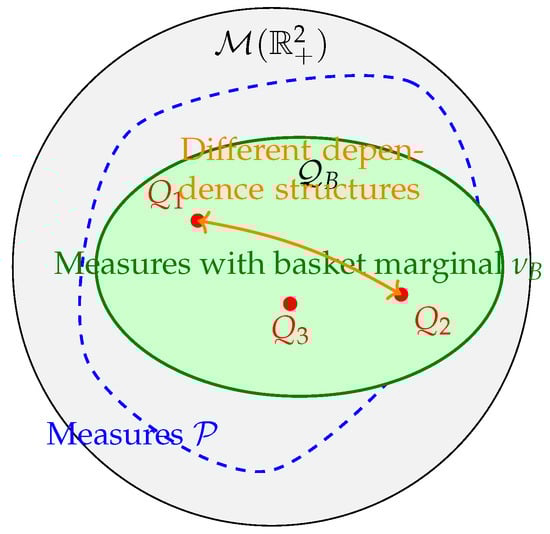
Figure 1.
Conceptual illustration: The space of probability measures on . We consider the subset of measures consistent with no-arbitrage and the subset having the correct basket marginal distribution . Their intersection contains multiple measures (points like ), all consistent with basket prices but differing in dependence structure and pricing of other derivatives.
Proof.
Convexity: Let and . Consider . Since is convex, . For any , the linearity of the integral implies:
Thus, , proving convexity.
Weak* closedness: For fixed , the functional is continuous with respect to the weak* topology. The set is the pre-image of a closed set under a continuous map, hence weak* closed. Since , it is an intersection of weak* closed sets and thus itself weak* closed.
Non-singleton nature: The calibration condition for all is equivalent to fixing the marginal distribution of the basket random variable under Q. Let this fixed distribution be denoted by .
However, knowing the distribution of does not determine the joint distribution of . This is a manifestation of the problem of reconstructing a joint distribution from its projections, related to Sklar’s theorem and copula theory (Nelsen 2006; Sklar 1959). Sklar’s theorem states that joint distributions can be decomposed into marginal distributions and a copula capturing dependence. Here, basket calibration fixes only one linear projection , leaving the dependence structure largely undetermined. There can be infinitely many joint distributions that induce the same marginal distribution for the basket variable but differ in their dependence structure. The existence of such distinct measures compatible with market incompleteness ensures that contains more than one element. □
Theorem 1 establishes that multiple probability measures can fit the observed basket prices. The critical question remains whether these distinct measures yield identical prices for best-of options.
4. Incompatibility of Payoff Functions via Extreme Ray Theory
The potential for non-uniqueness arises from the difference between the payoff functions and . We formalize this difference using the theory of convex functions, particularly the concept of extreme rays. Let denote the cone of continuous convex functions . A non-zero function generates an extreme ray if with implies and for some .
4.1. Intuitive Explanation for Non-Technical Readers
The mathematical concept of “extreme rays” provides a geometric way to understand why basket and best-of options are fundamentally incompatible. Think of payoff functions as shapes in mathematical space:
- Basket payoffs create “wedge-shaped” regions—imagine a piece of pie cut from a circular plate.
- Best-of payoffs create “L-shaped” regions—like the corner of a rectangular room.
The extreme ray theory proves that L-shaped regions cannot be built by combining wedge-shaped pieces, no matter how cleverly you arrange them. This geometric impossibility underlies the economic impossibility of perfectly hedging best-of options using only basket instruments. This intuition explains why practitioners observe persistent model risk in exotic derivatives: the mathematical structures are genuinely incompatible, not merely difficult to calibrate.
4.2. Mathematical Foundation
The extreme ray characterization relies on the fundamental geometric properties of convex functions. In the cone , a function generates an extreme ray if it cannot be decomposed into a sum of other non-proportional elements of the cone. This property is preserved under positive scalar multiplication but not under genuine convex combinations.
Theorem 2
(Johansen (1974)). A polyhedral convex function generates an extreme ray in the cone of convex functions on if and only if, at each vertex of its epigraph, exactly three affine pieces (faces) meet.
Proposition 1 (Payoff Function Structures).
- (i)
- The basket call payoff does not generate an extreme ray.
- (ii)
- For , the best-of call payoff generates an extreme ray in the cone of convex functions on .
This geometric incompatibility—formalized through extreme ray theory—underlies the impossibility of expressing one in terms of the other, as visualized in Figure 2 which shows the distinct payoff profiles for basket and best-of options.
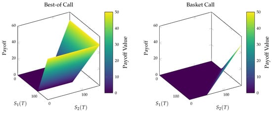
Figure 2.
Payoff profiles for options on two assets () with strike . (Left): Call on the best-of, . (Right): Call on a basket, . The best-of call payoff generates an extreme ray of the cone of convex functions on , while the basket call payoff is convex but not an extreme ray.
Proof.
(i) The function is the maximum of two affine functions: and . Non-differentiability occurs where , i.e., along the line . Along this line, only these two affine pieces define the function. It does not satisfy the three-face condition of Theorem 2.
(ii) The function is where , , and . The critical edge in its epigraph is the line . Along this edge (for ), three faces of the epigraph meet: , , and . This configuration satisfies the condition of Theorem 2, confirming that generates an extreme ray. □
This difference in geometric structure leads to linear independence.
Theorem 3 (Linear Independence of Payoffs).
For , the best-of payoff function cannot be represented as a finite positive linear combination of basket payoff functions plus an affine term. That is, there do not exist , , and constants such that:
Proof.
Suppose such a representation (4) exists. The right-hand side is a finite positive linear combination of basket payoff functions (which do not generate extreme rays by Proposition 1(i)) plus an affine term. By properties of convex combinations in the cone of convex functions, such combinations cannot generate an extreme ray.
However, Proposition 1(ii) establishes that generates an extreme ray for . This contradiction proves no such representation exists.
Geometric Intuition: Basket payoffs create “wedge-shaped” regions (half-spaces above lines ), while best-of payoffs create “L-shaped” regions. This fundamental geometric incompatibility—formalized through extreme ray theory—underlies the impossibility of expressing one in terms of the other. □
This linear independence is key: if cannot be built from payoffs, then knowing the expectations of (i.e., basket prices) should not be sufficient to determine the expectation of (the best-of option price).
5. Construction of Distinct Equivalent Measures with Different Best-Of Prices
We now explicitly construct two distinct equivalent measures, and , both belonging to , but yielding different prices for the best-of option. Recall that if and only if the law of under Q is the market-implied distribution . For each z in the support of , consider the line segment: .
Theorem 4 (Existence of Distinct Equivalent Measures with Different Best-of Prices).
Assume and let be a non-degenerate basket distribution. Then there exist distinct equivalent probability measures such that:
- (i)
- Both reproduce the basket distribution for .
- (ii)
- for appropriate .
Proof.
Construction: For each , define conditional measures on the line segment using a parameter , . We define two measures and by specifying their conditional distributions on and integrating against .
- For Measure (inducing ), the conditional measure on consists of mass at and mass at .
- For Measure (inducing ), the conditional measure on consists of mass at and mass at .
These measures are then formed by integrating these conditional allocations over all z with respect to .
Verification:
- Equivalence: Both and assign positive mass to the same set of points, namely . Since , both measures assign positive probability to these points and zero probability elsewhere. Thus, they have the same null sets and are equivalent (mutually absolutely continuous). Explicitly:
- Basket Consistency: For any measurable set A, the probability of the basket value being in A is . For both and , all the constructed mass for a given basket value z lies on the line where . The total conditional mass on is for , and for . Integrating over all z with respect to shows that both measures reproduce as the distribution of the basket variable.
- Different Best-of Expectations: Let’s compute the price of the best-of option under each measure.
Since and we chose , the coefficients for the terms and are different in the two integrals. The functions and are linearly independent. Therefore, unless is degenerate in a way that makes the integrals equal for all K, the expectations will differ. The non-equality follows, establishing that two equivalent measures can yield different best-of option prices while maintaining identical basket calibration.
□
Figure 3 provides a schematic representation of these two extreme joint distributions, illustrating how different mass allocations along the constraint lines lead to distinct dependence structures while maintaining identical basket marginals.
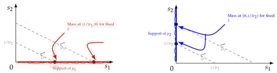
Figure 3.
Schematic representation of two extreme joint distributions, (left) and (right), compatible with a given distribution of the basket value . The dashed lines represent level sets . For a fixed z, the conditional mass of is concentrated at on the -axis (red), while the conditional mass of is concentrated at on the -axis (blue).
Remark: If , symmetry implies regardless of . Non-uniqueness requires asymmetric weights.
6. Range of Best-Of Option Prices and No-Arbitrage Bounds
Since the best-of option price is not uniquely determined by basket calibration, it is natural to ask for the range of possible prices consistent with the observed basket market.
Theorem 5 (Range of Best-of Option Prices).
For each , the set of possible prices for the best-of call option, consistent with the market basket prices, is a closed interval . That is,
where and . Furthermore, if is non-degenerate and , then .
Proof.
The set is convex (Theorem 1). The pricing functional is linear. The image of a convex set under a linear map is convex, which in must be an interval. Since is weak* closed and is weak* continuous, the interval is closed. The fact that follows directly from Theorem 4, which showed the existence of with .
The bounds can be characterized explicitly. To minimize subject to and , we choose and to be as close as possible, which leads to if possible. This yields the lower bound:
To maximize subject to , we make one variable as large as possible by setting the other to zero. This corresponds to the measures constructed in Section 5 and gives the upper bound:
Since and are all different (assuming ), the functions inside the integrals are distinct, confirming that for non-degenerate distributions . □
6.1. Bounds Under Equivalent Measure Constraints
When restricting to the set of equivalent measures , the bounds are:
The parametric construction in Theorem 4 demonstrates that , establishing non-uniqueness even under equivalence constraints. We have the relationship .
6.2. Tightness Characterization
The bounds and represent theoretical extremes. The upper bound is achieved by non-equivalent measures (Dirac masses concentrated on the axes), while the lower bound corresponds to a measure where all mass lies on the line . Equivalent measures, such as those constructed in Theorem 4, yield prices strictly within the interval , with the exact position determined by the parameter . This demonstrates that equivalence constraints reduce but do not eliminate fundamental model uncertainty.
7. Synthesis, Implications, and Extensions
7.1. Model Risk Visualization
This theorem quantifies the model risk inherent in pricing best-of options using only basket calibration. The bounds established in Theorem 5 provide a rigorous quantification of this model risk, as illustrated in Figure 4, where the uncertainty interval varies with strike price K.
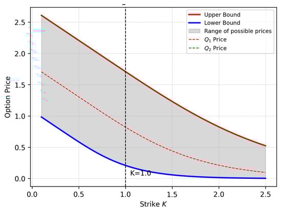
Figure 4.
Model Risk Visualization: The graph illustrates how the uncertainty interval for best-of option prices varies with strike price K. The shaded region represents fundamental model risk that cannot be eliminated through improved calibration to basket options alone. The width quantifies inherent uncertainty practitioners must manage.
7.2. Financial Implications: From Mathematical Theory to Trading Practice
7.2.1. Quantifying Fundamental Model Risk
The interval represents irreducible uncertainty that persists regardless of calibration sophistication or computational resources. This provides the first rigorous quantification of what practitioners have long recognized intuitively: exotic derivative pricing contains fundamental, model-dependent uncertainty that cannot be eliminated through better calibration techniques alone.
7.2.2. Specific Risk Management Applications
- Model Validation and Sanity Checks: Use bounds as theoretical benchmarks for best-of option pricing models. Any model producing prices outside these intervals indicates potential arbitrage opportunities or fundamental errors. This can be implemented as an automatic model validation criterion in risk management systems, complementing existing numerical pricing methodologies (Henry-Labordère 2013).
- Trading and Market Making Protocols: Bid-ask spreads should reflect this fundamental model uncertainty. Position limits and mark-to-market tolerance ranges can be scaled based on the width of the uncertainty interval.
- Regulatory Capital and Risk Assessment: The uncertainty range provides a defensible basis for allocating additional model risk capital. Stress tests should include scenarios that span the theoretical uncertainty bounds.
7.2.3. Market Incompleteness and Information-Theoretic Perspective
The non-uniqueness reflects fundamental information limitations rather than calibration failures. Even with perfect basket option data and unlimited computational power, the joint distribution of remains mathematically underdetermined. To reduce this ambiguity, calibration must incorporate instruments that provide complementary information, such as options on individual assets (to fix marginals) and derivatives explicitly sensitive to correlation or extremal co-movements (e.g., spread options).
7.3. Extensions and Future Research
Our analysis focuses on equivalent probability measures consistent with basket option prices. Several important extensions merit further investigation.
7.3.1. Equivalent Martingale Measure Constraints
The additional requirement that measures satisfy the martingale property introduces further technical complexity. Recent computational advances in martingale optimal transport (Guo and Obłój 2019) suggest promising avenues for numerical implementation while preserving the fundamental theoretical insights. Schrödinger bridges and entropic regularization methods Guyon (2022), provide computational frameworks for addressing such constraints. Entropic regularization adds a convex penalty term, making the problem computationally tractable, often via Sinkhorn-type algorithms. These techniques allow for the numerical computation of martingale measures, with neural network approaches (Eckstein and Kupper 2019) providing promising computational frameworks, preserving our fundamental non-uniqueness results within a more constrained, risk-neutral setting.
7.3.2. Additional Research Directions
- Multi-Asset Framework: Extension to assets introduces additional complexity in characterizing extremal measures and computing bounds.
- Market Data Implementation: Real market data contains noise and discrete strike grids, requiring robust numerical methods for bound computation.
- Dynamic Framework: Incorporating dynamic hedging considerations and transaction costs into the theoretical framework.
- Empirical Validation: Testing the theoretical bounds against observed market spreads for best-of and basket options.
The connection to optimal transport theory suggests that our framework could be extended to other incomplete market problems where partial information about multivariate distributions creates fundamental pricing ambiguities.
8. Conclusions
This paper has established that perfect calibration to basket call option prices is insufficient to uniquely determine the price of a best-of call option in a two-asset model. We demonstrated that the set of equivalent probability measures consistent with basket prices contains measures that yield different best-of option prices, and we derived the tight no-arbitrage bounds for these prices. The core insight is that basket options only constrain the risk-neutral distribution along one dimension (the weighted sum), leaving significant freedom in the specification of the joint distribution, particularly concerning the dependence structure which critically impacts the best-of option price. Our findings quantify inherent model risk, illustrate market incompleteness, provide valuable no-arbitrage bounds, and inform calibration strategies. The result highlights the fundamental limitations in inferring multivariate dependencies from prices of derivatives based on linear combinations of the underlying assets.
The mathematical framework developed here contributes to the broader literature on model uncertainty and incomplete markets, with applications extending beyond option pricing to any context involving partial information about multivariate distributions. The connection to optimal transport theory through Schrödinger bridges suggests promising avenues for computational implementation while preserving the fundamental theoretical insights.
Author Contributions
Conceptualization, M.A.; methodology, M.A. and A.G.; software, L.E. All authors have read and agreed to the published version of the manuscript.
Funding
This research received no external funding.
Data Availability Statement
Data sharing not applicable to this article as no datasets were generated or analysed during the current study.
Conflicts of Interest
The authors declare no conflict of interest.
References
- Ang, Andrew, and Joseph Chen. 2002. Asymmetric correlations of equity portfolios. Journal of Financial Economics 63: 443–94. [Google Scholar] [CrossRef]
- Ballotta, Laura, Griselda Deelstra, and Grégory Rayée. 2014. Extracting the Implied Correlation from Quanto Derivatives. Working Paper. Bruxelles: Université Libre de Bruxelles. [Google Scholar]
- Breeden, Douglas T., and Robert H. Litzenberger. 1978. Prices of state-contingent claims implicit in option prices. The Journal of Business 51: 621–51. [Google Scholar] [CrossRef]
- Chen, Yongxin, Tryphon T. Georgiou, and Michele Pavon. 2021. Optimal transport over a linear dynamical system. IEEE Transactions on Automatic Controlt 66: 2137–52. [Google Scholar] [CrossRef]
- Cont, Rama, Romain Deguest, and Yu Hang Kan. 2010. Inverse problems in option pricing: Extracting model parameters from market data. SIAM Journal on Financial Mathematics 20: 173–80. [Google Scholar]
- Coqueret, Guillaume, and Bertrand Tavin. 2020. A note on implied correlation for bivariate contracts. Economics Bulletin 40: 1388–96. [Google Scholar]
- Da Fonseca, José, Martino Grasselli, and Claudio Tebaldi. 2007. Option pricing when correlations are stochastic: An analytical framework. Review of Derivatives Research 10: 151–80. [Google Scholar] [CrossRef]
- De March, Hadrien, and Nizar Touzi. 2019. Irreducible convex paving for decomposition of multidimensional martingale transport plans. The Annals of Probability 47: 1726–74. [Google Scholar] [CrossRef]
- Derman, Emanuel, and Iraj Kani. 1994. Riding on a smile. Risk 7: 32–39. [Google Scholar]
- Driessen, Joost, Pascal J. Maenhout, and Grigory Vilkov. 2009. The price of correlation risk: Evidence from equity options. The Journal of Finance 64: 1377–406. [Google Scholar] [CrossRef]
- Dupire, Bruno. 1994. Pricing with a smile. Risk 7: 18–20. [Google Scholar]
- Eckstein, Stephan, and Michael Kupper. 2019. Computation of optimal transport and related hedging problems via penalization and neural networks. Applied Mathematics & Optimization 80: 639–67. [Google Scholar]
- Fu, Jason. 2019. Worst-of Options Pricing and Implied Correlation Using Copula Methods. Master’s Thesis, Princeton University, Princeton, NJ, USA. [Google Scholar]
- Guo, Gaoyue, and Jan Obłój. 2019. Computational methods for martingale optimal transport problems. The Annals of Applied Probability 29: 3311–47. [Google Scholar] [CrossRef]
- Guyon, Julien. 2022. The joint calibration of SPX and VIX options with log-affine SLV models. Quantitative Finance 22: 1661–84. [Google Scholar]
- Henry-Labordère, Pierre. 2013. Automated option pricing: Numerical methods. International Journal of Theoretical and Applied Finance 16: 1350042. [Google Scholar] [CrossRef]
- Hobson, David, Peter Laurence, and Tai-Ho Wang. 2005. Static-arbitrage upper bounds for the prices of basket options. Quantitative Finance 5: 329–42. [Google Scholar] [CrossRef]
- Johansen, Soren. 1974. The extremal convex functions. Mathematica Scandinavica 34: 61–68. [Google Scholar] [CrossRef]
- Kremens, Lukas, and Ian Martin. 2019. The quanto theory of exchange rates. American Economic Review 109: 810–43. [Google Scholar] [CrossRef]
- Laurence, Peter, and Tai-Ho Wang. 2008. Sharp upper and lower bounds for basket options. Applied Mathematical Finance 15: 97–133. [Google Scholar]
- Léonard, Christian. 2014. A survey of the Schrödinger problem and some of its connections with optimal transport. Discrete & Continuous Dynamical Systems 34: 1533–74. [Google Scholar]
- Nelsen, Roger B. 2006. An Introduction to Copulas, 2nd ed. New York: Springer Science & Business Media. [Google Scholar]
- Peyré, Gabriel, and Marco Cuturi. 2019. Computational optimal transport: With applications to data science. Foundations and Trends® in Machine Learning 11: 355–607. [Google Scholar] [CrossRef]
- Romo, Jacinto Marabel. 2012. Worst-of options and correlation skew under a stochastic correlation framework. International Journal of Theoretical and Applied Finance 15: 47–54. [Google Scholar]
- Sklar, Abe. 1959. Fonctions de répartition à n dimensions et leurs marges. Publications de l’Institut Statistique de l’Université de Paris 8: 229–31. [Google Scholar]
Disclaimer/Publisher’s Note: The statements, opinions and data contained in all publications are solely those of the individual author(s) and contributor(s) and not of MDPI and/or the editor(s). MDPI and/or the editor(s) disclaim responsibility for any injury to people or property resulting from any ideas, methods, instructions or products referred to in the content. |
© 2025 by the authors. Licensee MDPI, Basel, Switzerland. This article is an open access article distributed under the terms and conditions of the Creative Commons Attribution (CC BY) license (https://creativecommons.org/licenses/by/4.0/).