Policy Implications and Risk Mitigation of Greenhouse Gas Management in the Renewable Energy Sector

Abstract

The transition toward renewable energy systems offers significant opportunities to reduce greenhouse gas (GHG) emissions, while also introducing new challenges in risk management and policy design. This study examines the long-term effects of renewable energy consumption, the risk factors associated with environmental taxation, and public expenditure on greenhouse gas (GHG) emissions across 27 European Union countries over a period of 22 years. Using panel data techniques—specifically the Fully Modified Ordinary Least Squares (FMOLS) and Dynamic Ordinary Least Squares (DOLS) estimators—the analysis identifies robust cointegrating relationships among environmental, fiscal, and energy variables. The joint null hypothesis (H₀) states that renewable energy consumption, environmental taxation, and public environmental expenditure do not exert a statistically significant negative long-run effect on greenhouse gas (GHG) emissions in the European Union (i.e., none of these variables contributes to reducing GHG emissions in the long run). The findings show that renewable energy consumption and environmental taxes significantly and negatively affect GHG emissions, confirming their effectiveness as instruments for emission risk mitigation. Pollution taxes display the strongest elasticity among fiscal measures, indicating their pivotal role in carbon reduction strategies. Furthermore, public expenditure, particularly in waste management, meaningfully contributes to long-term emission reductions. These results highlight that a cohesive policy framework combining renewable energy development, targeted taxation, and strategic public investment can effectively minimize the environmental and economic risks associated with decarbonization. The study provides valuable empirical evidence for policymakers and risk analysts, underscoring the importance of integrated fiscal and energy policies in achieving sustainable climate risk management across the European Union

1. Introduction

Greenhouse gas (GHG) emissions continue to shape the global environmental policy agenda, particularly as climate change mitigation efforts intensify. Greenhouse gas emissions, especially carbon dioxide and methane, trap heat in the atmosphere, causing the phenomenon of increasing Earth temperatures. Limiting GHG emissions is considered crucial for mitigating the severe consequences of climate change, such as rising sea levels, threats to natural ecosystems, and increased extreme weather events that cause significant damage to the economy, infrastructure, and human health. The main sources of GHG emissions are transportation, electricity production, industry, commercial and residential energy consumption, agriculture, land use, and forestry.

To mitigate the effects, a growing body of the literature highlights the role of renewable energy, environmental taxation, and government expenditure in reducing emissions and promoting sustainable development (Shafiei and Salim 2014; Anisiuba et al. 2023). However, divergent results persist regarding the magnitude and direction of these effects, reflecting the complex interplay between environmental interventions and macroeconomic dynamics (Jenkins et al. 2016; Batra 2023).

While many studies confirm a negative association between renewable energy consumption and GHG emissions, the role of environmental taxation and public expenditure remain debated. For example, authors such Bashir et al. (2020), Cadoret et al. (2020), Abbas et al. (2025), and Khan et al. (2025) are arguing that taxation schemes may incentivize clean technology adoption, whereas Hao (2022) and Alsagr and van Hemmen (2021) suggest their efficiency is contingent upon sectoral alignment and institutional quality.

At the same time, Serrano and Zaveri (2020) emphasize that socio-political participation significantly shapes the success of energy transitions, while Lennon and Dunphy (2024) advocate for inclusive governance frameworks to promote equitable decarbonization.

This study addresses these debates and fills this well-known research gap by investigating the long-term effects of renewable energy, environmental taxes, and public expenditure on GHG emissions across the 27 European Union countries over 22 years. It contributes to the empirical literature by applying robust cointegration techniques (FMOLS and DOLS) to a balanced panel dataset and identifying policy variables with the greatest mitigation potential.

To achieve its final goal, the current research is organized into five chapters. The first two chapters, Introduction and Literature Review, are mainly theoretical, focusing on previous research in the field and the main models used by other authors. Based on these findings, the authors developed and applied a specific research model in the third chapter, Data and Methodology. The main results of the case study are presented in the fourth chapter, Empirical Results. The final chapter, Conclusions, presents the main findings of this study, demonstrating that renewable energy consumption, environmental taxation, and public environmental expenditure all have statistically significant long-term negative effects on GHG emissions in the European Union, thereby mitigating the risk of exacerbating negative environmental impacts.

2. Literature Review

The literature on environmental policy and greenhouse gas (GHG) emissions within renewable energy reveals a complex interaction between regulation, technology, and market forces. Effective policies must integrate renewable technologies while addressing socio-economic factors to ensure both sustainability and equity (Jenkins et al. 2016; Batra 2023). Adanma and Ogunbiyi (2024) argue that, to enhance the synergy between environmental sustainability and economic growth, stakeholders must incorporate technological advancement, foster global partnerships, and adopt an integrated policy framework.

Renewable integration enhances energy security, reduces fossil fuel dependence, and stimulates clean technology innovation. Incentives and regulatory frameworks foster investment in renewables, generating economic opportunities and reducing emissions (Shafiei and Salim 2014; Anisiuba et al. 2023). At the same time, policies that promote diversification and stakeholder engagement increase transparency, legitimacy, and long-term success (Jenkins et al. 2016). Investment in environment-related R&D expenditure must accompany environmental taxes in order to be effective (Dahmani 2023).

Regional examples highlight how governance structures shape outcomes. The EU’s coordinated decarbonization approach illustrates the effectiveness of harmonized legislation (Szulecki and Claes 2019). In contrast, studies in China and emerging markets emphasize the need for locally responsive, sector-specific strategies (Hao 2022; Alsagr and van Hemmen 2021). Financial systems and environmental taxation also enable sustainable energy adoption (Bashir et al. 2020; Cadoret et al. 2020; Abbas et al. 2025; Khan et al. 2025). One study shows that lobbying negatively affects the transition towards renewable energy production, while increasing awareness is the main positive factor (Marra and Colantonio 2022).

Industrial applications show that renewable energy adoption fosters both emissions reductions and economic synergies, as seen in eco-industrial parks and industrial symbiosis models (Butturi et al. 2019). Likewise, technological innovation—including R&D and blockchain—plays a critical role in advancing efficiency and transparency (Xu and Khan 2023; Rejeb et al. 2024). Khan et al. (2025) emphasize the role of innovative technologies in improving non-renewable energy resource efficiency and mitigating greenhouse gas emissions. Since energy production accounts for almost 60% of GHG emissions, special focus should be placed on increasing renewable energy production (Al-Shetwi 2022). The implementation of green policies is creating a spillover effect, resulting in “regional green development efficiency” (Ding et al. 2022) and increased life expectancy in certain regions (Fan et al. 2025). Hoang et al. (2021) analyze the issues faced by the integration of renewable resources in smart cities. Public awareness and societal participation are equally vital. Social media shapes perceptions of renewables and pressures policymakers to act (Zhang et al. 2022). Inclusive governance ensures policies align with local needs and promote equity in energy transitions (Lennon and Dunphy 2024). International cooperation and knowledge-sharing further enhance adoption and emissions reductions (Szulecki and Claes 2019; Huttmanová and Mikča 2024). Overall, the literature emphasizes that renewable energy transitions must balance innovation, governance, and social inclusion. Robust frameworks combining incentives, regulation, stakeholder collaboration, and international coordination are essential for achieving climate goals and advancing sustainable development (Maevsky et al. 2024; Byrareddy et al. 2023). A positive correlation is observed between the adoption of renewable energy and GDP, industrial productivity, and the implementation of technological innovation, especially in regions with access to abundant renewable resources (Chou et al. 2023; Saquib et al. 2023; Socci et al. 2023).

Specific models to analyze the impact of digital economy implementation and the transition to renewable energy have been developed by Hwang (2023) and tested across 18 Latin American and Caribbean countries.

When assessing policy implications, several studies (such as Wills et al. 2021) consider carbon pricing policies more effective than command-and-control policies. Local social and political conditions, and the combination of economic measures and taxation, must be carefully considered before implementing a carbon tax (Criqui et al. 2019). Corvino (2023) proposes a global scheme of CO₂ taxation with the redistribution of carbon revenues to support climate justice. Cohesive policy frameworks, not just traditional fiscal measures, must be implemented to address structural interdependencies (Kanayo et al. 2025).

The main risks undermining the implementation of GHG reduction strategies by switching to renewable energy in certain industries are considered to be high initial investment costs, low levels of technical ability, and high maintenance costs (Pouresmaieli et al. 2023; Corvino 2023). In addition, the implementation of aggressive carbon pricing policies can negatively affect low-income households, exacerbating energy poverty and creating a need for compensation mechanisms and exemptions for certain sectors to mitigate these effects (Wills et al. 2021; Dahmani 2023; Huttmanová and Mikča 2024; Kanayo et al. 2025).

Concerns about reduced economic competitiveness in certain industries and regions can impede the successful implementation of GHG strategies (Criqui et al. 2019; Socci et al. 2023; Gong and Huo 2024). Economic uncertainty can also hinder the process of effective GHG taxation (Abbas et al. 2025). While most authors support the GHG taxation system, several studies question its efficiency and environmental impact (Liobikienė et al. 2019; Zhang et al. 2020). Under certain conditions, high environmental taxes can decrease GDP, increase costs, raise unemployment, and hinder economic growth (Nagovnak et al. 2024; Usman et al. 2025). Integrated measures and dynamic tax models are proposed to increase effectiveness (Gong and Huo 2024).

Taking the above into consideration, the current study intends to examine the long-term effects of renewable energy consumption and public expenditure on greenhouse gas (GHG) emissions, as well as the risk factors of environmental taxation, across 27 European Union countries over a period of 22 years.

3. Data and Methodology

The reviewed literature employs a diverse range of methodologies to analyze the effects of taxation and environmental policies on greenhouse gas (GHG) emissions. These can be broadly categorized into econometric models, economy-wide simulation models, and qualitative or comparative analyses: Autoregressive Distributed Lag Models (Kanayo et al. 2025; Abbas et al. 2025), Regression Models (Zhang et al. 2020; Socci et al. 2023; Khan et al. 2025), Generalized Method of Moments, and Nonlinear and Quantile Models (Fan et al. 2025), Computable General Equilibrium (Wills et al. 2021) Models, and Comparative and Qualitative Analyses (Criqui et al. 2019). Most authors using qualitative models also employed quantitative methods such as Dynamic Ordinary Least Squares (D.O.L.S.) and Fully Modified Ordinary Least Squares (F.M.O.L.S.) models, which were also employed by us, while in the methodology selection we employed unit root and cointegration tests. A summary of the main qualitative methods employed is provided in

Table 1. Summary of main methods employed in the literature.

Authors	Methods Employed
Kanayo et al. (2025); Abbas et al. (2025)	Autoregressive Distributed Lag Models
Zhang et al. (2020); Socci et al. (2023); Khan et al. (2025)	Regression Models
Fan et al. (2025)	Generalized Method of Moments, and Nonlinear and Quantile Models
Wills et al. (2021)	Computable General Equilibrium
Criqui et al. (2019)	Models, and Comparative and Qualitative Analyses

.

3.1. Independent Panel Unit Root Tests Framework

To check if series are stationary, panel unit roots must be applied; usually, tests are used for this (BDt, Cht, HTt, Imt, Let—see Abbreviations).

The basic approach determines whether there are restrictions on the auto-regressive process (as in (1)) across the cross-sections or series.

$$y_{it}={\rho }_i{y}_{it-1}+X_{it}{\delta }_i+{ϵ}_{it}$$

(1)

where y_it is the dependent variable, X_it is the independent variables matrix, and ϵ_it is the idiosyncratic error.

Based on these restrictions, one can impose ρ_i = ρ for all i if |ρ_i| = 1, meaning that y_i has a unit root.

The LLCt, BDt, and Ht tests assume a common unit root, meaning that ρ_i is identical across cross-sections. LLCt and Brt consider a basic ADF, as in (2), with the null H₀ as in (3), and the alternative written as (4).

$$\mathsf{\Delta }{y}_{it}=\alpha y_{it-1}+\sum _{j=1}^{p_i} {\beta }_{ij}\mathsf{\Delta }{y}_{it-j}+X_{it}^{\prime }\delta +{ϵ}_{it}$$

(2)

$$H_0:\alpha =0$$

(3)

$$Ha:{\alpha }_i\le 0$$

(4)

An alternative methodology was developed by IPSt, as well as the Fisher–ADF and Fisher–PP tests. These tests all allow for individual unit root processes, meaning that the presence of a unit root can vary across cross-sections.

Equation (5) uses the null H₀ in (6) and Ha in (7).

$$\mathsf{\Delta }{y}_{it}={\alpha }_i{y}_{it-1}+\sum _{j=1}^{p_i} {\beta }_{ij}\mathsf{\Delta }{y}_{it-j}+X_{it}^{\prime }\delta +{ϵ}_{it}$$

(5)

$$H_0:{\alpha }_i=0,\mathrm{for}\mathrm{all}i$$

(6)

$$H_1:\left\{\begin{array}{cc}{\alpha }_i=0& \mathrm{for}i=\mathrm{1,2},\dots ,N_1\\ {\alpha }_i<0& \mathrm{for}i=N+1,N+2,\dots ,N\end{array}\right.$$

(7)

The empirical findings from these tests are discussed in detail in Section 4.

3.2. FMOLS and DOLS Characteristics

The ‘fully modified’ OLS (FMOLS) estimator, introduced by Pedroni (2001) and Phillips and Moon (1999), is a non-parametric approach that accounts for possible endogeneity and serial correlation. Based on the general model specified in Equation (8), and the cointegrating relationship described in Equation (9), the FMOLS estimator of β is obtained as shown in Equation (10); see Pedroni (2001) and Pedroni (2004).

$$y_{it}={\alpha }_i+\beta x_{it}+{\mu }_{it}$$

(8)

$$x_{it}=x_{it-1}+{\epsilon }_{it}$$

(9)

$$\begin{array}{cc}{\widehat{\beta }}_{\mathrm{FMOLS}}=& {\left({\displaystyle \sum _{i=1}^N} {\widehat{L}}_{22i}^{-2}{\displaystyle \sum _{t=1}^T} {\left(x_{it}-{\overline{x}}_i\right)}^2\right)}^{-1}\hfill \\ & \times {\displaystyle \sum _{i=1}^N} {\widehat{L}}_{11i}^{-1}{\widehat{L}}_{22i}^{-1}\left({\displaystyle \sum _{t=1}^T} \left(x_{it}-{\overline{x}}_i\right)y_{it}^{*}-T{\widehat{\delta }}_i\right)\hfill \end{array}$$

(10)

where

$$y_{it}^{*}=\left(y_{it}-{\widehat{y}}_i\right)-\left({\displaystyle \frac{{\widehat{L}}_{21i}}{{\widehat{L}}_{22i}}}\right)\mathsf{\Delta }{X}_{it}\left({\displaystyle \frac{{\widehat{L}}_{21i}-{\widehat{L}}_{22i}}{{\widehat{L}}_{22i}}}\right)\beta \left(x_{it}-{\overline{x}}_i\right)$$

(11)

$${\widehat{\delta }}_i={\widehat{\mathsf{\Gamma }}}_{21i}+{\widehat{\mathsf{\Omega }}}_{21i}^0-\left({\displaystyle \frac{{\widehat{L}}_{21i}}{{\widehat{L}}_{22i}}}\right)\left({\widehat{\mathsf{\Gamma }}}_{22i}+{\widehat{\mathsf{\Omega }}}_{22i}^0\right)$$

(12)

A general representation, as is largely presented in the literature (e.g., the DOLS methodology in (Mark and Sul 2003)), is available in Equation (13).

$$y_{it}={\alpha }_i+{\lambda }_{i}t+{\theta }_t+{\underset{\_}{\gamma }}^{\prime }{\underset{\_}{x}}_{it}+u_{it}^{†}$$

(13)

where α_i represents an individual-specific effect, λ_it is an individual-specific linear trend, θ_t denotes a common time-specific factor, and $u_{it}^{†}$ is the idiosyncratic error term, which is independent across individuals i, but may exhibit dependence across time t.

The simplest model, which imposes the restrictions λ_i = 0 and θ_t = 0 for all i and t, is employed to analyze the relationships among the variables of interest—ghg, rec, tax tenv, tax poll, exp envpr, exp wm, exp wwm, and exp poll ab—as specified in Equation (14).

$$y_{it}={\alpha }_i+{\underset{\_}{\gamma }}^{\prime }{\underset{\_}{x}}_{it}+u_{it}^{†}$$

(14)

To address potential endogeneity, under the assumption that there is a correlation with v_it, the variable is projected onto the leads and lags of p_i, as outlined in (15).

$$u_{it}^{†}=\sum _{s=-p_i}^{p_i} {\underset{\_}{\delta }}_{i,s}^{\prime }{\underset{\_}{v}}_{it-s}+u_{it}=\sum _{s=-p_i}^{p_i} {\underset{\_}{\delta }}_{i,s}^{\prime }\mathsf{\Delta }{\underset{\_}{x}}_{it-s}+u_{it}={\underset{\_}{\delta }}_i^{\prime }{\underset{\_}{z}}_{it}+u_{it}$$

(15)

Substituting the projection, and taking the time-series averages, the new equation is (16).

$${\displaystyle \frac{1}{T}}\sum _{t=1}^T y_{it}={\alpha }_i+{\underset{\_}{\gamma }}^{\prime }{\displaystyle \frac{1}{T}}\sum _{t=1}^T {\underset{\_}{x}}_{it}+{\delta }_i^{\prime }{\displaystyle \frac{1}{T}}\sum _{t=1}^T {\underset{\_}{z}}_{it}+{\displaystyle \frac{1}{T}}\sum _{t=1}^T u_{it}$$

(16)

The selection of the long-run effects methodology is motivated by several key considerations: economic and environmental variables—such as GDP, GDP per capita, CO₂ emissions, and GHG—typically exhibit unit roots, as widely documented in the literature; traditional fixed and random effects estimators often yield biased coefficients due to the non-stationarity of variables in levels; and the non-stationary variables are found to be cointegrated (see Section 4). The empirical analysis of tests and results, in the context of risk mitigation and “anti-risk” instruments, focuses on the long-run hypotheses (the primary interest lies in the sign and significance of the estimated coefficients), as shown below:

• Renewable energy consumption (REC)

H₀. 

β_REC ≥ 0 (renewable energy consumption does not reduce or may increase GHG emissions).

H₁. 

β_REC < 0 (renewable energy consumption significantly reduces GHG emissions).

B.

Environmental taxation (ETAX)

H₀. 

β_ETAX ≥ 0 (environmental taxes have no reducing effect on GHG emissions).

H₁. 

β_ETAX < 0 (environmental taxes significantly reduce GHG emissions).

C.

Public environmental protection expenditure (ENVEXP)

H₀. 

β_ENVEXP ≥ 0 (public environmental spending does not reduce or may increase GHG emissions).

H₁. 

β_ENVEXP < 0 (public environmental expenditure significantly reduces GHG emissions).

The joint null hypothesis that none of the three policy instruments contributes to long-run GHG mitigation is as follows:

H₀. 

β_REC ≥ 0, β_ETAX ≥ 0, β_ENVEXP ≥ 0.

All three individual and joint null hypotheses are strongly rejected, confirming the effectiveness of renewable energy promotion, environmental taxation, and targeted public environmental spending as long-term GHG mitigation tools in the European Union.

3.3. Data Description

The data was obtained from the World Bank database. Summary statistics are available in

Table 2. Summary statistics.

	Mean	SD	Min	Max	N
ghg	9.1320	4.5835	0.7000	26.5000	594
rec	17.1911	11.7787	0.0900	58.4000	594
tax tenv	9.9705	15.1171	0.1546	58.6630	594
tax poll	0.2684	0.4830	0.0004	2.7510	594
exp envpr	3.2586	5.2591	0.0181	22.0830	594
exp wm	1.3917	2.5625	0.0047	11.2890	594
exp wwm	0.7128	1.2091	0.0004	4.9740	572
exp poll ab	0.4622	0.8205	0.0001	4.0520	572

Source: author’s calculation.

.

The dataset consists of 594 observations spanning 22 years, covering the period from 2000 to 2021 (with data extracted in January 2025) and includes 27 European Union countries as the panel units. The dependent variable, representing environmental impact, is Greenhouse Gas Emissions (GHG), the primary control variable is renewable energy consumption (rec), and the first proxy for taxation is environmental taxation—tax tenv. To ensure the reliability and comparability of the panel dataset, only variables with complete observations across all 27 EU member states for the period 1995–2022 were retained for the main estimations, resulting in a balanced panel of 594 observations for the core variables (GHG emissions, renewable energy consumption, total environmental tax revenue, pollution-specific tax revenue, total environmental protection expenditure, and waste-management expenditure). Two supplementary expenditure sub-categories (wastewater management and pollution abatement) had minor missing values and were therefore used mainly in robustness checks (N = 572).

To mitigate the influence of extreme outliers—common in fiscal and environmental expenditure series—all variables (in levels and logs where applicable) were winsorized at the 1st and 99th percentiles using Stata’s winsor2 command with the cuts (1 99) option. This procedure reduces the distorting effect of extreme values while preserving the original sample size and economic meaning of the data. After winsorizing, the summary statistics reported in Table 2 were calculated.

4. Empirical Results

Our dataset is classified in the econometric literature as panel time series data—panel data with a sufficiently long-time dimension to be treated as a time series—which often exhibit unit roots. Conducting unit root tests is essential to avoid spurious regression. All econometric analyses were performed using Stata 16.0. Specifically, panel unit root tests (IPS, Fisher-type), Pedroni and Westerlund cointegration tests (including the command xtcointtest and its variants for different model specifications), ARDL/PMG estimations (xtpmg, AIC with a maximum of four lags), FMOLS and DOLS estimations (xtcointreg), winsorizing (winsor2), and VIF calculations (reg, vif) were conducted in Stata. Therefore, our initial data analysis focused on testing for the presence of unit roots. We applied the IPS and Fisher tests, with the results for the dependent variable GHG in levels presented in

Table 3. Unit root test results for GHG variable in levels, Series: GHG, levels.

Method	Statistic	Prob.	Cross-Sections	Obs
LLC t	0.22948	0.5908	27	540
IPSt W-stat	2.01199	0.9779	27	540
ADF Chi-square	46.1753	0.7666	27	540
PP Chi-square	44.6226	0.8147	27	567

Source: author’s calculation.

.

The results of the unit root tests (see Table 3) indicate that, since all probability values in the Prob column exceed 0.1, the null hypothesis of a unit root cannot be rejected. This implies that the GHG variable is non-stationary in levels. However, for the first difference, all Prob values are 0.000 (see

Table 4. Unit root test results for the GHG variable in first difference.

Method	Statistic	Prob.Cross-Sections	Obs
LLCt t	−8.65377	0.0000	27
IPSt W-stat	−10.5041	0.0000	27
ADF-Chi-square	212.292	0.0000	27
PP-Chi-square	411.803	0.0000	27

Source: author’s calculation.

), leading to the rejection of the null hypothesis. Therefore, the dependent variable GHG is integrated of order one, I(1). Similar results were found for the other variables, all of which are I(1), with details provided in

Table A1. Summary of unit root tests results for all variables.

Variables	r (zttildebar)	r (P)	r (L)	r (Z)	r (Pm)
rec	−0.6342	37.8570	0.1364	0.1574	−1.5534
d.rec	−8.4827	360.5376	−18.3755	8.9887	29.4966
tax tenv	1.0869	35.4213	0.6395	0.6947	−1.7877
d.tax tenv	15.7263	3.7132	9.8169	8.9887	−4.8388
tax poll	22.8609	0.1727	7.6310	6.5975	−5.1795
d.tax poll	2.0322	322.3567	−15.8774	−7.7043	25.8226
exp envpr	−3.0313	70.8677	−2.6031	−2.8241	1.6231
d.exp envpr	−5.9339	272.4474	−13.0263	−8.9944	21.0201
exp wm	0.9733	58.9131	0.7837	0.1519	0.4728
d.exp wm	−4.7766	222.3016	−10.5757	−8.3733	16.1948

Source: author’s calculation.

. In summary, the unit root tests confirm that the GHG series contains a unit root in levels but becomes stationary after first differencing. The unit root tests for the other variables yield comparable findings, as evidenced by the LLCt, IPSt, ADF and PP-Fisher Chi-square tests, all showing non-stationarity in levels and stationarity in first differences.

The second set of tests refer to the existence of cointegration between the dependent variable and independent variables. We present a simplified table cointegration between the dependent variable (GHG) and the first proxy for environmental taxation. A more analytic table is available in Appendix A (see

Table A2. Initial VIF—all variables.

	VIF	1/VIF
exp envpr	23.61	0.04
rec	1.12	0.89
exp wm	11.34	0.09
tax tenv	8.66	0.12
tax poll	1.41	0.71
exp wwm	1.27	0.79
exp poll ab	1.23	0.81
Mean VIF	6.95

Source: author’s calculation.

).

The cointegration analysis shows that the Kao test rejects the null hypothesis of no cointegration in three out of five panel statistics. Similarly, the Pedroni test rejects the null hypothesis across all three panel specifications, indicating cointegration among the variables. The Westerlund test also rejects the null at the 0.01% significance level, further confirming the presence of cointegration. Overall, most tests reject the null hypothesis, demonstrating that the variables are cointegrated and move together in the long run. Given this evidence of cointegration, the robustness of the study is enhanced, allowing us to apply the FMOLS and DOLS estimators. The estimation results for the cointegrating relationship between GHG, rec, environmental taxation, and expenditure are presented in

Table 5. Testing cointegration between variables.

Variables Name:	ghg, tax tenv
Test name:	Kao
MDF t	2.9297
DF t	3.392
ADF t	3.6373
UMDF t	0.8982
UDF t	1.0872
Test name	Pedroni
MPP t	3.5377
PP t	5.1084
ADFt	6.0562
Test name	Westerlund
Variance ratio	4.6868

Source: author’s calculation.

. Panel Dynamic Ordinary Least Squares (DOLS) is an effective method for estimating cointegrating vectors in panel data, but it requires the variables to be cointegrated.

We found that in all the implied tests (Kao, Pedroni, and Westerlund), with the null hypothesis of no cointegration, the results of seven of nine statistics are significant at the 1% level. The null hypothesis for most of the models are rejected in specified tests, so we can conclude that the variables greenhouse gas emissions (GHG) and environmental total taxation (tax tenv) are cointegrated. The cointegration tests for the other variables yield similar results (corresponding findings are available upon request). In summary, none of the variables are integrated of the order two, I(2). The presence of I(1) variables, along with evidence of long-run relationships among them, justifies the use of FMOLS and DOLS estimators, confirming that the chosen methodologies are appropriate.

The chosen variables are related to the scope of the paper, the theoretical background on environmental taxes, and the existing literature (Zhang et al. 2020; Socci et al. 2023; Khan et al. 2025).

As the initial Variance Inflation Factor (VIF) test for the full model (when all variables are used, see Table A2) is 6.95, above 5 (the threshold recommended by the existing literature (e.g., Chatterjee and Simonoff (2013), Marcoulides and Raykov (2019)), we decided to use each tax and expenditure separately, as a proxy for environmental policy. In this approach, there were no identified problems. For all of the implied models, the VIFs means are under 5. (The outcome for the first model is available in Appendix A. The calculus is accessible in

Table A3. First model VIF.

	VIF	1/VIF
rec	1.02	0.98
tax tenv	1.02	0.98
Mean VIF	1.02

Source: author’s calculation.

—the VIF result is 1.02, with the other results being available on demand.)

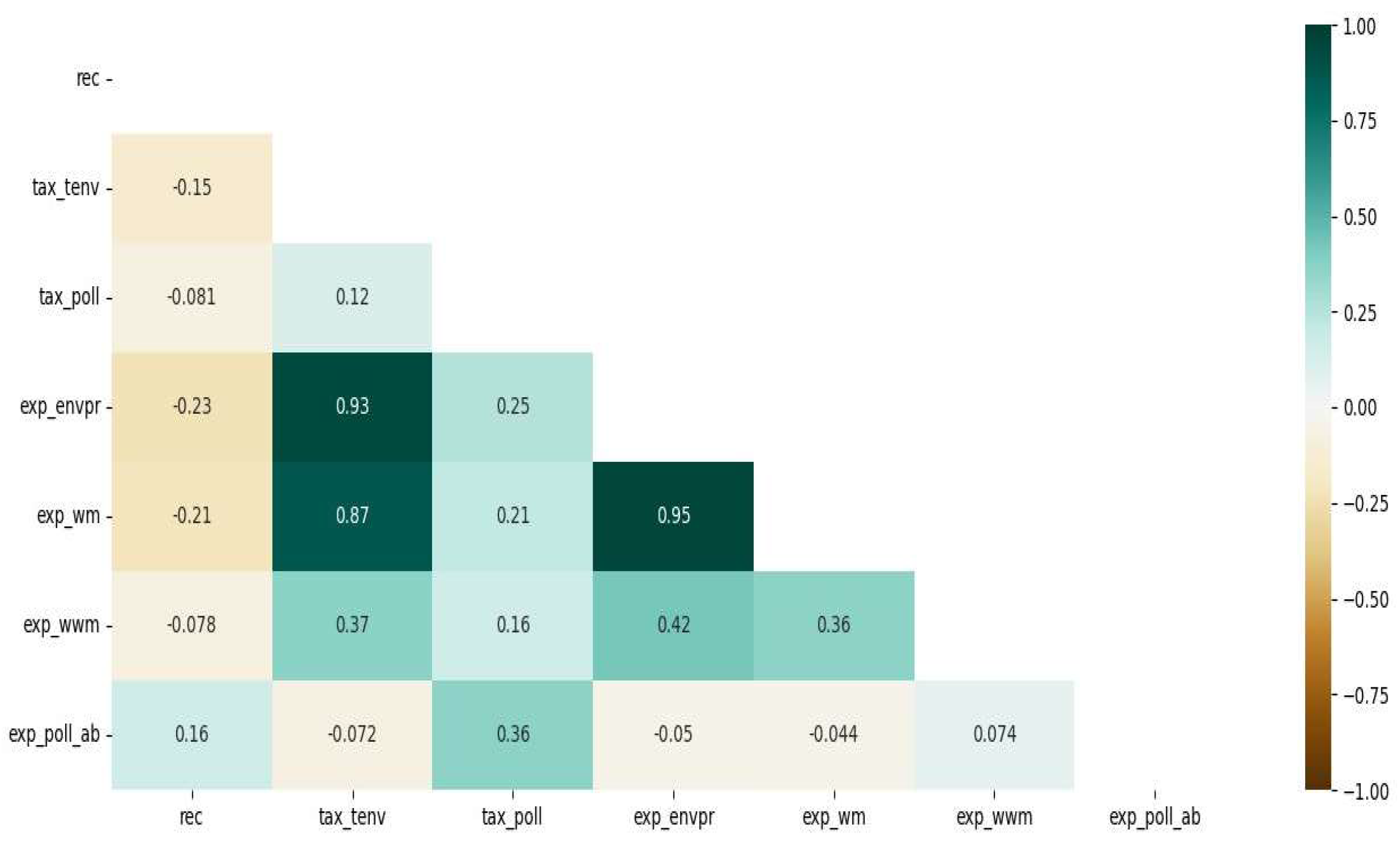
The previous findings are graphically presented by the correlation matrix, in which we can describe the independent variables used as a proxy for environmental policy as highly correlated (see Figure 1).

The initial analysis used Renewable Energy (rec) as a control variable, in conjunction with the variables of interest—the total environmental taxes (tax tenv) and pollution taxes (tax poll)—applying FMOLS and DOLS methodologies (using Driscoll–Kraay standard errors, which are robust to cross-sectional dependence, heteroskedasticity, and autocorrelation). The calculus was performed in four models, available in

Table 6. Effects of taxation; dependent variable: GHG.

Model No.:	1	2	3	4
Method:	FMOLS	DOLS	FMOLS	DOLS
REC	−0.1699	−0.1310	−0.1701	−0.1162
	(0.0191)	(0.0252)	(0.0190)	(0.0253)
TAXTENV	−0.0619	−0.1061
	(0.0360)	(0.0511)
TAX POLL			−0.7597	−1.3241
			(0.3164)	(0.4841)
R-sq.:	0.9366	0.9663	0.9368	0.9716

Source: author’s calculation.

. The impact of renewable energy (rec) is found to be negative, as expected; the coefficients vary between −0.1701 and −0.1162, and the highest effect encountered in the FMOLS model in conjunction with pollution taxes (tax tpol). All of the implied coefficients are statistically significant at least at the 10% level. The econometric interpretation is that a one-unit increase in renewable energy has the effect of decreasing greenhouse gas emissions by 0.17 units in the long run, ceteris paribus.

Regarding the influence of taxation, both of the proxies have a negative effect on GHG, with the highest impact being detected in the DOLS model (column four in Table 5). The coefficients vary between −1.3241 and −0.0619, being statistically significant at least at the 10% level. We interpret the results as suggesting that a long-term increase in pollution tax by one unit decreases greenhouse gas emissions by 1.32 units, ceteris paribus.

Our results are consistent with those of Bashir et al. (2020), Cadoret et al. (2020), Abbas et al. (2025), and Khan et al. (2025), who find that financial systems and environmental taxation act as enablers of sustainable energy adoption. A positive correlation is observed between the adoption of renewable energy and GDP, industrial productivity, and the implementation of technological innovation, particularly in regions with access to abundant renewable resources (Chou et al. 2023; Saquib et al. 2023; Socci et al. 2023).

The consequence of expenditure was quantified using four proxies: exp envpr, exp wm, exp wm, exp poll ab. The results for the first two proxies are available in

Table 7. Effects of environmental expenditure (1) on dependent variable GHG.

Model No.:	5	6	7	8
Method:	FMOLS	DOLS	FMOLS	DOLS
REC	−0.1663	−0.1202	−0.1720	−0.1361
	(0.0187)	(0.0231)	(0.0184)	(0.0237)
EXP ENVPR	−0.1981	−0.3285
	(0.0774)	(0.1198)
EXP WM			−0.2905	−0.4080
			(0.1261)	(0.1740)
R-sq.:	0.9378	0.9656	0.9375	0.9642

Source: author’s calculation.

, showing the same negative impact on GHG, as expected. The control variable is maintained at rec, confirming the inverse effect. The coefficients of rec are between −0.1720 and −0.1202, being close in value to those in previous models The highest value of all coefficients is met in model No. 7 (with the independent variables being rec and exp wm). The econometric explanation is the same as in former models (1–4). The impact of expenditure is also negative, as expected; the coefficients for proxies are (−0.4080, −0.1981), being statistically significant by at least 10%. We can conclude that the effect of environmental expenditure is negative, as expected, with the highest reduction in GHG being calculated in model no. 8 using DOLS methodology: a one-unit increase in waste management expenditure (exp wm) will decrease greenhouse gas emissions (GHG) by 0.4 units, on average, in the long term, ceteris paribus.

For the last two proxies used to assess the impact of environmental expenditure, the coefficients are not statistically significant, excepting model 11 for pollution expenditure, obtained using FMOLS methodology. The results are available in Appendix A, in

Table A4. Effects of environmental expenditure (2) on dependent variable GHG.

Model No.:	9	10	11	12
Method:	FMOLS	DOLS	FMOLS	DOLS
REC	−0.1923	−0.1535	−0.1826	−0.1730
	(0.0185)	(0.0229)	(0.0184)	(0.0230)
EXP_WWM	−0.2570	−0.0415
	(0.3904)	(0.5757)
EXP POLL AB			−0.5571	−0.5134
			(0.2349)	(0.2883)
R-squared:	0.9392	0.9671	0.9390	0.9669

Source: author’s calculation.

.

The impact of renewable energy is negative and statistically significant at least at the 10% level (same table; first row of results).

As observed, the quantitative methods used in this study validated those initially presented in the literature review and methodology regarding ARDL/PMG estimations, including the methods presented by Kanayo et al. (2025), Abbas et al. (2025), Zhang et al. (2020), Socci et al. (2023), and Khan et al. (2025).

Our results are consistent with other studies in the field (Shafiei and Salim 2014; Anisiuba et al. 2023), which find that incentives and regulatory frameworks promote investment in renewables, generate economic opportunities, and reduce emissions.

A positive correlation is observed between the adoption of renewable energy and GDP, industrial productivity, and the implementation of technological innovation, especially in regions with access to abundant renewable resources (Chou et al. 2023; Saquib et al. 2023; Socci et al. 2023).

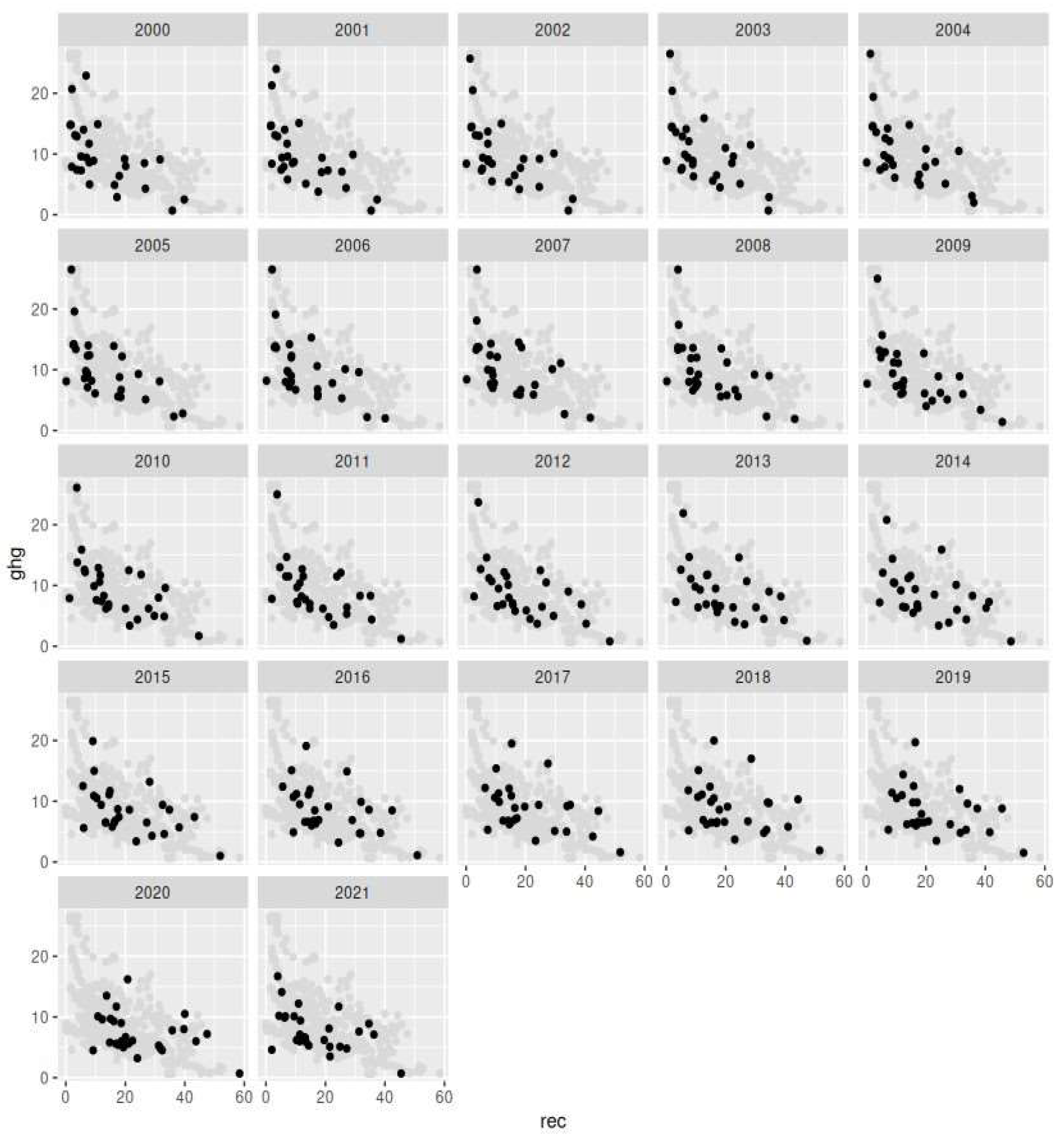
The study also supports research on interdependencies (Kanayo et al. 2025) that considers that cohesive policy frameworks, not just traditional fiscal measures, must be implemented to address structural interdependencies. Based on this research, we also consider our study to align with the findings of Bashir et al. (2020), Cadoret et al. (2020), Abbas et al. (2025), and Khan et al. (2025), who suggest that financial systems and environmental taxation also enable sustainable energy adoption. The results are further supported by the visualization of our data (see Figure 2), where it is evident across all panels (countries) that rec growth on the X axis determines the GHG reduction on the Y axis.

We conclude that renewables, taxes, and environmental expenditure have positive effects on GHG reduction (as indicated by the negative coefficients). Therefore, decisions regarding environmental policy—such as increasing the proportion of renewable energy combined with the use of environmental taxation and expenditure as part of fiscal and budgetary policies—should be reconsidered.

5. Conclusions

The findings of this study demonstrate that renewable energy consumption, environmental taxation, and public environmental expenditure all exert statistically significant long-term negative effects on GHG emissions in the European Union, mitigating the risk of the exacerbation of negative influences on environment. Among these, renewable energy is a consistent driver of emission risk reduction, supporting the previous literature that links clean energy expansion with environmental sustainability. The empirical evidence indicates that, on average, a one-unit increase in renewable energy usage is associated with a 0.17-unit decrease in GHG emissions, with other factors remaining constant, in terms of risk becoming an instrument of risk control.

Environmental taxation also has a substantial impact, with pollution-specific taxes producing the strongest effects. The elasticity results show that a one-unit increase in pollution tax can reduce GHG emissions by up to 1.32 units in the long run. These results confirm that fiscal instruments, when appropriately targeted, can influence environmental behavior and outcomes, reducing the amplification of risk.

Furthermore, the analysis reveals that public expenditure, particularly in waste management, is an effective tool for GHG risk mitigation. Although not all types of expenditure demonstrate the same level of efficacy, those linked to pollution control and environmental programs contribute meaningfully to reducing the risk of emissions.

These findings have important implications for policymakers and risk analysts and risk mitigation. A multipronged strategy that combines investments in renewable energy infrastructure with targeted environmental taxation and well-designed public expenditure programs can deliver measurable reductions in emissions. Policymakers should ensure that such instruments are tailored to national contexts and aligned with broader climate objectives. Additionally, the research highlights the value of an empirical policy evaluation to guide evidence-based decision-making in environmental governance. Risk environmental analysts should also consider such valuable instruments in future risk management plans.

Despite the robustness of the findings, certain limitations persist. While FMOLS and DOLS estimators address endogeneity to some extent, potential reverse causality and omitted variables, such as technological innovation, green technology trade, or other interactions (i.e., European Union Emissions Trading System—EUETS) remain unaccounted for. Moreover, the use of aggregate public environmental expenditure data may mask variations in effectiveness across categories and member states. Future research could overcome these constraints by employing an instrumental variable or system GMM estimations, utilizing disaggregated expenditure data for longer time periods, incorporating spatial econometric models, and exploring the mediating roles of green innovation and carbon pricing mechanisms.

In conclusion, this study demonstrates that economic policies shape environmental risks through both direct channels (e.g., carbon pricing, energy subsidies, and pollution taxes that immediately alter emission intensities) and indirect pathways (mediated by income growth, technological diffusion, trade openness, and structural transformation), highlighting the need for an integrated policy design that simultaneously targets emission sources and the broader macroeconomic transmission mechanisms to achieve effective and sustainable environmental outcomes. Variables not included in the present analysis will be examined in future research.