Optimal Investment Considerations for a Single Cohort Life Insurance Portfolio

Abstract

This study examines the portfolio optimization problem of an insurance company that issues an annuity, receives the associated premiums as a lump sum, and invests in a financial market. The insurer’s objective is to determine an investment strategy that minimizes the likelihood of defaulting on annuity payments before ceasing operations, where default occurs if the portfolio value, net of the annuity liability, becomes negative. Unlike the previous work, here the mortality intensity is stochastic and follows a Cox–Ingersoll–Ross (CIR) process. Dynamic programming is employed, and the value function is characterized by a Hamilton–Jacobi–Bellman (HJB) equation, and the former is linearized through the Legendre transform. Numerical results show that default probability declines with higher initial wealth and mortality intensity, while stochastic mortality volatility has little impact—though slightly higher volatility marginally reduces default risk. Optimal stock investment falls with increasing wealth and mortality intensity, and is nearly constant for low wealth levels. Mortality volatility has minimal influence, but a higher Sharpe ratio raises optimal investment, underscoring the role of risk-adjusted returns.

1. Introduction

The foundations of dynamic portfolio management in continuous stochastic settings were laid by Merton (1969) and Merton (1971), with Karatzas (1989) providing a comprehensive treatment of continuous-time portfolio choice. The problem of minimizing the probability of ruin was first addressed in discrete time by Ferguson (1965) and later extended to continuous-time diffusion models by Browne (1995), who showed that the strategy minimizing ruin probability also maximizes exponential utility. In the non-life insurance context, the portfolio selection problem, aimed at minimizing ruin probability and encompassing consumption, investment, and reinsurance decisions, has been studied extensively, including in Bayraktar et al. (2008); Liang and Young (2018); Luo and Taksar (2011); Promislow and Young (2005); Schmidli (2002).

Our work builds on the framework of Browne (1995) but introduces two key innovations. First, we incorporate required benefit payments to annuitants directly into the portfolio dynamics. Second, we model mortality intensity as a stochastic process, specifically in continuous time, within the portfolio selection problem of a life insurer.

For life insurers, sustaining the ability to meet long-term obligations, particularly the timely payment of claims and benefits, is of paramount importance. Regulatory frameworks such as Solvency II and risk-based capital (RBC) regimes require insurers to hold reserves that ensure solvency with high probability, accounting for both market and longevity risks. This motivates our portfolio-wide perspective, in contrast to works such as Christiansen and Fahrenwaldt (2016) and Hinkkanen (2022), which focus on individual contracts and solvency considerations related to contract design.

The study most closely related to ours is Cahyaningtias et al. (2023), which examines the portfolio problem of an insurer issuing an annuity, receiving the premium as a lump sum, and investing in a financial market. In their model, mortality intensity is assumed to be either constant or a Brownian motion with drift. In contrast, we adopt a more realistic specification in which mortality intensity follows a Cox–Ingersoll–Ross (CIR) process. The aim of this paper is to analyze how introducing a realistic stochastic mortality intensity model, articulated by a Cox–Ingersoll–Ross process, affects the insurer’s optimal investment strategy and solvency outcomes compared to the framework of Cahyaningtias et al. (2023).

In continuous-time mortality modeling, the CIR process serves as a model for the instantaneous mortality intensity. It captures both time dependence and stochastic variability in mortality trends while, unlike the Ornstein–Uhlenbeck process, guaranteeing non-negativity. The use of the CIR process in mortality modeling was first explored by Dahl (2004), Luciano and Vigna (2005, 2008), and has since been applied in various contexts, including Blackburn and Sherris (2013); Jevtić and Regis (2019, 2021); Luciano et al. (2012), and De Rosa et al. (2021). To the best of our knowledge, this is the first study to apply the CIR process in the portfolio optimization problem of a life insurer.

Incorporating stochastic mortality introduces additional realism and complexity into the insurer’s portfolio optimization problem. Unlike an additional stochastic interest rate factor, stochastic mortality directly determines the timing and magnitude of insurance liabilities, altering both asset and liability dynamics, a dimension that, to our knowledge, has not been previously analyzed in this optimization context. From a technical perspective, it increases the dimensionality of the stochastic control system, making the corresponding Hamilton–Jacobi–Bellman (HJB) equation analytically intractable. To address this, we apply a duality approach in which the problem is reformulated through a dual value function that satisfies a linear partial differential equation. Other approaches such as Markov chain approximations (see Bayraktar et al. 2011) may be employed to tackle this problem as well.

Our main contributions are threefold. First, we derive appropriate boundary conditions for this dual formulation and prove that the dual value function is concave, allowing recovery of the original value function through the Legendre transform. Second, we introduce a numerically stable and convergent scheme for solving the resulting PDE. Third, we demonstrate that the CIR-based framework yields quantitatively different and more realistic predictions than deterministic or Brownian mortality models, with direct implications for capital adequacy and optimal investment under longevity uncertainty. The framework provides a theoretical foundation for understanding prudential investment behavior and state-dependent reserve requirements in life insurance portfolios.

The remainder of the paper is organized as follows. Section 2 presents the model setup, while Section 3 introduces the research objective and formulates the optimization problem. Section 4 describes the numerical analysis approach, and Section 5 reports the results of various numerical experiments. Section 6 concludes the paper.

2. Model Setup

Let ${\{(W(t),B(t))\}}_{t\in [0,\infty )}$ be a two-dimension Brownian motion on a probability space $(\Omega ,{\{{\mathcal{F}}_t\}}_{t\in [0,\infty )},\mathcal{F},\mathbb{P}).$ The filtration $\{{\mathcal{F}}_t\}$ is the completed filtration generated by $\{(W(t),$${B(t))\}}_{t\in [0,\infty )}.$ Without loss of generality, we consider a simple financial market consisting of a savings account with interest rate $r=0.$ This can be achieved by taking the zero-coupon bond as numéraire. Another financial instrument available for trading is a stock whose dynamics are driven by a geometric Brownian motion $W(t)$ to model the underlying uncertainty of this risky asset with drift $\mu$ and volatility $\sigma >0$ as follows

$$dS(t)=S(t)(\mu dt+\sigma dW(t)).$$

Suppose that an insurance company issues an annuity with payment rate $K,$ i.e., at time t, the insurance company has to pay out $KI(t)dt$, where $I(t)$ denotes the proportion of clients who are alive at time t. The premiums are collected as a lump-sum at a time prior to $t=0$ and from this time onward, we only consider payout phase with no restriction of time horizon for the sake of simplicity. Without loss of generality, we assume that initially there is a unit mass of insureds with identical characteristics (one cohort) that buy one unit of annuity. Following Luciano and Vigna (2005), and other works in continuous time mortality modeling, we assume that the stochastic mortality intensity ${\{\lambda (t)\}}_{t\in [0,\infty )}$ follows a CIR process

$$d\lambda (t)=A\lambda (t)dt+\delta \sqrt{\lambda (t)}dB(t),$$

for some positive parameters A and $\delta .$ The Brownian motion $B(t)$ is used to model the underlying uncertainty of mortality intensity. A strictly positive and exponentially increasing mortality intensity means that as a life ages, the instantaneous hazard rate, i.e., the probability of dying in the next infinitesimal time interval, increases over time. This is not only biologically plausible but necessary: without an increasing hazard rate, individuals would have a positive probability of surviving indefinitely, which is clearly unrealistic.

Let $I(t)$ be the proportion of insureds who are alive at time t, hence

$$I(t)=e^{-{\int }_0^t\lambda (u)du}.$$

Let x be the initial wealth that the company holds to service future payment. Then, the payment fund is maintained by a portfolio consisting of risky and risk-free assets. Its dynamics are given by

$$dX(t)=\pi (t)X(t)(\mu dt+\sigma dW(t))-K{e}^{-{\int }_0^t\lambda (u)du}dt,X(0)=x,$$

where $\pi (t)$ denotes the proportion of wealth invested in the stock at time $t.$ The wealth dynamics when parameterized through $\Delta (t),$ i.e., the number of stocks held at time t in the portfolio is

$$dX(t)=\Delta (t)S(t)(\mu dt+\sigma dW(t))-K{e}^{-{\int }_0^t\lambda (u)du}dt,X(0)=x.$$

(1)

Let $Y(t)=X(t)e^{{\int }_0^t\lambda (u)du},$ then by the stochastic product rule we have that

$$dY(t)=[(\lambda (t)+\mu \pi (t))Y(t)-K]dt+\sigma \pi (t)Y(t)dW(t),Y(0)=X(0)=x.$$

(2)

Suppose that ${\tau }_d$ is the random time when the company stops operating. This time can also represent the switching of managers, random default time, new regulations, etc. Also, assume that ${\tau }_d$ is exponentially distributed with intensity $\gamma$. Finally, let us denote ${\tau }_0$ as the first time when the insurance company cannot meet its obligation, i.e.,

$${\tau }_0:=inf\{s\ge 0:X(s)=0\}=inf\{s\ge 0:Y(s)=0\}.$$

3. Objective and Optimization Problem

We are ready at this point to formulate our objective. The company tries to select a portfolio to minimize the probability of being unable to make payments before it stops operating, i.e.,

$$\underset{\pi }{inf}P[{\tau }_0\le {\tau }_d|Y(0)=y,\lambda (0)=\lambda ].$$

Remark 1.

Let us point out that this portfolio problem is scaling invariant. Indeed, let $X(t)$ be the wealth process of (1) and $\widehat{X}(t)$ be the wealth with $\widehat{X}(0)=MX(0)$ for some positive constant M and $\widehat{\Delta }(t)=M\Delta (t),$ i.e., the number of stocks held in the portfolio scaled by a factor M. Then if the annuity $\widehat{K}$ is also scaled, i.e., $\widehat{K}=MK$, then it is clear that $d\widehat{X}(t)=MdX(t)$; thus, $\widehat{X}(t)=MX(t).$ Moreover $inf\{s\ge 0:X(s)=0\}=inf\{s\ge 0:\widehat{X}(s)=0\}.$

Also, let us note that given the dynamics of ${\{S(t)\}}_{t\in [0,\infty )}$ and ${\{\lambda (t)\}}_{t\in [0,\infty )},$ this problem is time homogeneous, i.e.,

$$V(x,\lambda )=\underset{\pi }{inf}P[{\tau }_0\le {\tau }_d|Y(s)=x,\lambda (s)=\lambda ],$$

regardless of time s.

3.1. HJB Equation

By using the Dynamic Programming Principle (DPP) we obtain the following Hamilton–Jacobi–Bellman (HJB) equation for the value function $V(x,\lambda )$

$$\gamma V=(\lambda x-K)V_x+A\lambda V_{\lambda }+{\displaystyle \frac{1}{2}}{\delta }^2\lambda V_{\lambda \lambda }+\underset{\pi }{min}\{\mu x{V}_x\pi +{\displaystyle \frac{1}{2}}{\sigma }^2{V}_{xx}{x}^2{\pi }^2\},$$

(3)

with boundary condition $V(0,\lambda )=1.$ Indeed, since ${\tau }_d$ is exponentially distributed with intensity $\gamma ,$ it follows that

$$P[{\tau }_0\le {\tau }_d]=E[exp(-\gamma {\tau }_0)].$$

We employ the martingale optimality principle (see Pham 2009, p. 102) to characterize the value function. The HJB Equation (3) states that $exp(-\gamma t)V\left(Y(t),\lambda (t)\right)$ is a submartingale, and a martingale for the optimal $({\pi }^{*},Y^{*}).$ Indeed, Itô’s Lemma applied to $(exp(-\gamma t))V(Y(t),\lambda (t))$ yields

$$\begin{array}{c}\mathrm{d}\left(exp(-\gamma t)V\left(Y(t),\lambda (t)\right)\right)=exp(-\gamma t){\mathcal{A}}^{\pi }V\left(Y(t),\lambda (t)\right)+exp(-\gamma t)V_{\lambda }\left(Y(t),\lambda (t)\right)\delta \sqrt{\lambda (t)}\mathrm{d}B(t)+\\ exp(-\gamma t)V_y\left(Y(t),\lambda (t)\right)\sigma \pi (t)Y(t)\mathrm{d}W(t),\end{array}$$

where the operator ${\mathcal{A}}^{\pi }$ is defined by having

$${\mathcal{A}}^{\pi }V(x,\lambda )=(\lambda x-K)V_x+A\lambda V_{\lambda }+{\displaystyle \frac{1}{2}}{\delta }^2\lambda V_{\lambda \lambda }+\{\mu x{V}_x\pi +{\displaystyle \frac{1}{2}}{\sigma }^2{V}_{xx}{x}^2{\pi }^2\}-\gamma V.$$

The claim follows since ${\mathcal{A}}^{\pi }V\ge 0$ and ${\mathcal{A}}^{{\pi }^{*}}V=0$.

Thus,

$$\begin{array}{c}V\left(Y(0),\lambda (0)\right)\le E\left[exp(-\gamma {\tau }_0)V\left(Y({\tau }_0),\lambda ({\tau }_0)\right)\right]=\\ E\left[exp(-\gamma {\tau }_0)V\left(0,\lambda ({\tau }_0)\right)\right]=E\left[exp(-\gamma {\tau }_0)\right]=P\left[{\tau }_0\le {\tau }_d\right]\end{array}$$

whence the optimality,

$$\begin{array}{c}V\left(Y(0),\lambda (0)\right)=E\left[exp(-\gamma {\tau }_0)V\left(Y({\tau }_0^{*}),\lambda ({\tau }_0^{*})\right)\right]=\\ E\left[exp(-\gamma {\tau }_0^{*})V\left(0,\lambda ({\tau }_0^{*})\right)\right]=E\left[exp(-\gamma {\tau }_0^{*})\right]=P\left[{\tau }_0^{*}\le {\tau }_d\right]\end{array}$$

The optimizer in (3), given the convexity of V in x, is

$${\pi }^{*}=-{\displaystyle \frac{\mu V_x}{{\sigma }^{2}x{V}_{xx}}}.$$

(4)

The HJB equation is then rewritten as

$$\gamma V=(\lambda x-K)V_x+A\lambda V_{\lambda }+{\displaystyle \frac{1}{2}}{\delta }^2\lambda V_{\lambda \lambda }-{\displaystyle \frac{{\mu }^2{V}_x^2}{2{\sigma }^2{V}_{xx}}},$$

(5)

with boundary condition $V(0,\lambda )=1.$ Thus, the optimal proportion to be invested in the stock is

$${\pi }^{*}=-{\displaystyle \frac{\mu V_x}{{\sigma }^{2}x{V}_{xx}}},$$

and the optimal amount invested in the stock is

$${\Pi }^{*}=-{\displaystyle \frac{\mu V_x}{{\sigma }^2{V}_{xx}}}.$$

3.2. Fenchel–Legendre Transform

Let us introduce the Fenchel–Legendre transform of $V,$ denoted $w,$ by

$$w(y,\lambda )=\underset{x>0}{inf}[V(x,\lambda )+xy].$$

(6)

The function w is sometimes referred to as the dual function, and the following duality relationship holds

$$V(x,\lambda )=\underset{y>0}{sup}[w(y,\lambda )-xy].$$

(7)

In our analysis we work with the dual function w which is proved to be concave, and as such, the value function is obtained through (7) and it is convex.

The following first-order and second-order conditions hold

$$w_y(y,\lambda )=x,\mathrm{iff}{V}_x(x,\lambda )=-y,$$

(8)

$$w_{yy}(y,\lambda )=-{\displaystyle \frac{1}{V_{xx}(x,\lambda )}}.$$

Moreover, by differentiating with respect to $\lambda$ in (6) and (7), and using differentiation of the value function of an optimization problem, one gets

$$V_{\lambda }=w_{\lambda },V_{\lambda \lambda }=w_{\lambda \lambda }.$$

Thus, we arrive at the following PDE for w

$${\displaystyle \frac{{\mu }^2{y}^2}{2{\sigma }^2}}{w}_{yy}+{\displaystyle \frac{{\delta }^2}{2}}\lambda w_{\lambda \lambda }+(\gamma -\lambda )y{w}_y+A\lambda w_{\lambda }-\gamma w+Ky=0,$$

(9)

with the boundary conditions $w(0,\lambda )=0,w(\infty ,\lambda )=1.$ Let us justify these boundary conditions. It is clear that $w(0,\lambda )=0.$ Let us argue that $w(\infty ,\lambda )=1.$ It is obvious that $w(y,\lambda )\le 1$ by sending x to 0 in (6). For every $ϵ>0$ there is a sufficiently large $N>0$ such that ${inf}_{\frac{1}{N}>x>0}V(x,\lambda )\ge 1-ϵ,$ so $w(N,\lambda )>1-ϵ.$ Thus $w(\infty ,\lambda )=1.$ The boundary condition when $y=0$ is

$$w(y,0)=\underset{x>0}{inf}[exp(-\widehat{\beta }x)+xy]=\left\{\begin{array}{c}{\displaystyle \frac{y}{\widehat{\beta }}}-{\displaystyle \frac{y}{\widehat{\beta }}}ln\left({\displaystyle \frac{y}{\widehat{\widehat{\beta }}}}\right),y<\widehat{\beta }\hfill \\ 1,y\ge \widehat{\beta },\hfill \end{array}\right.$$

where $\widehat{\beta }=\left(\gamma +{\displaystyle \frac{{\mu }^2}{2{\sigma }^2}}\right){\displaystyle \frac{1}{K}},$ and it follows from Theorem 4.2 of Cahyaningtias et al. (2023). The existence of a solution for this elliptic PDE can be argued as in Chapter 4 of Krylov (1997).

The following theorem establishes the concavity in y for the dual value function w, which in turn yields the convexity of V in $x,$ (through (7)), and as such the candidate of (4) is indeed the optimizer.

Theorem 1.

The map $y\to w(y,\lambda )$ is concave.

Proof. 

Let us introduce the stochastic process $y(t)$ given by the SDE

$$dy(t)=y(t)\left((\gamma -\lambda (t))dt+{\displaystyle \frac{\mu }{\sigma }}dW(t)\right).$$

In fact

$$y(t)=y(0)exp\left({\int }_0^t\left(\gamma -\lambda (u)-{\displaystyle \frac{{\mu }^2}{2{\sigma }^2}}\right)du+{\displaystyle \frac{\mu }{\sigma }}W(t)\right).$$

(10)

 □

Then, the process

$$M(t)=exp(-(\gamma t))w(y(t),\lambda (t))+K{\int }_0^{t}y(u)du,$$

is a martingale. Let $\widehat{\tau }$ be the first time the process $\lambda (t)$ hits 0. Let us denote the function $w(y,0)$ as $F(y)$, i.e.,

$$F(y)=\left\{\begin{array}{c}{\displaystyle \frac{y}{\widehat{\beta }}}-{\displaystyle \frac{y}{\widehat{\beta }}}ln\left({\displaystyle \frac{y}{\widehat{\beta }}}\right),y<\widehat{\beta }\hfill \\ 1,y\ge \widehat{\beta },\hfill \end{array}\right.$$

which is a concave function in $y.$ Let us denote $y(0)=y,\lambda (0)=\lambda$; then, the martingale property of $M(t)$ yields

$$w(y,\lambda )=E\left[exp-(\gamma {\tau }_0)F(y(\widehat{\tau }))+K{\int }_0^{\widehat{\tau }}y(u)du\right].$$

The concavity of w in y yields from the concavity of F and the multiplicative dependence on the initial condition of the process $y(t)$ of (10). This completes the proof.

In light of the dual relationships, we can express ${\pi }^{*},{\Pi }^{*}$ in terms of the dual function.

$${\pi }^{*}=-{\displaystyle \frac{\mu }{{\sigma }^2{w}_y}}y{w}_{yy},$$

(11)

$${\Pi }^{*}=-{\displaystyle \frac{\mu }{{\sigma }^2}}y{w}_{yy}.$$

(12)

4. Numerical Analysis

We discretize the linear PDE in (9), with $y\in [0,\infty )$ and $\lambda \in [0,\infty )$:

$$\alpha y^2{w}_{yy}+\beta \lambda w_{\lambda \lambda }+(\gamma -\lambda )y{w}_y+A\lambda w_{\lambda }-\gamma w+Ky=0$$

(13)

using second-order accurate central differences (see LeVeque 2007), where $\alpha ={\mu }^2/(2{\sigma }^2)$ and $\beta ={\delta }^2/2$. Also, the original boundary conditions are

$$w(y=0,\lambda )=0,w(y=\infty ,\lambda )=1,w(y,\lambda =\infty )=0,$$

$$w(y,\lambda =0)=\left\{\begin{array}{cc}{\displaystyle \frac{y}{\eta }}\left(1-ln\left({\displaystyle \frac{y}{\eta }}\right)\right)\hfill & \mathrm{if}y<\eta \hfill \\ 1\hfill & \mathrm{if}y\ge \eta \hfill \end{array}\right.$$

where $\eta =(\alpha +\gamma )/K$. Note that the important range of $\lambda$ is $[0.05,0.2]$.

Computationally we will take $y\in [0,Y]$ and $\lambda \in [0,\Lambda ]$ where $Y\gg 1$ and $\Lambda \ge 1$, with $N\Delta y=Y$ and $N\Delta \lambda =\Lambda$. The boundary conditions become

$$w(y=0,\lambda )=0,w(y=Y,\lambda )=1,w(y,\lambda =\Lambda )=0,$$

$$w(y,\lambda =0)=\left\{\begin{array}{cc}{\displaystyle \frac{y}{\eta }}\left(1-ln\left({\displaystyle \frac{y}{\eta }}\right)\right)\hfill & \mathrm{if}y<\eta \hfill \\ 1\hfill & \mathrm{if}y\ge \eta \hfill \end{array}\right..$$

We label $w(y_i,{\lambda }_j)=w_{ij}$, with $i,j=1,\dots ,N+1$. Then the discrete equations for the linear PDE are

$$\alpha y_i^2{\displaystyle \frac{w_{i+1,j}-2w_{ij}+w_{i-1,j}}{\Delta y^2}}+\beta {\lambda }_j{\displaystyle \frac{w_{i,j+1}-2w_{ij}+w_{i,j-1}}{\Delta {\lambda }^2}}+$$

$$(\gamma -{\lambda }_j)y_i{\displaystyle \frac{w_{i+1,j}-w_{i-1,j}}{2\Delta y}}+A{\lambda }_j{\displaystyle \frac{w_{i,j+1}-w_{i,j-1}}{2\Delta \lambda }}-\gamma w_{ij}+K{y}_i=0.$$

(14)

Stacking the unknowns $w_{ij}$ for $i,j=2,\dots ,N$ into a vector $w_n$ for $n=1,\dots ,{(N-1)}^2$, we write the discrete equations as $Mw=b$, where b incorporates the boundary conditions. Due to the five-point stencil for second-order accurate central differences, M will be a banded matrix with five diagonals (main, sub- and super-diagonals, and sub- and super-fringes). This linear equation is then solved using a banded-matrix direct solve; LeVeque (2007).1

5. Numerical Experiments

In this section, we computed and plotted the probability of default and the corresponding optimal investment by using the following parameters: $x=y=[0,10]$, $\lambda =[0,0.5]$, $N_x=1000$, $N_y=100$, $N_{\lambda }=100$, $K=0.1$, $\gamma =0.001$, $\mu =0.15$, $\sigma =0.05$, $A=0.01$, and $\delta =0.005$.

Our choice of drift $\mu =0.15$ and volatility $\sigma =0.05$ parameters for the risky asset are stylized but intentionally chosen to represent an insurance company’s diversified investment portfolio rather than a single stock. Insurance portfolios typically consist of a dominant proportion of fixed income securities and equities, resulting in substantially lower aggregate volatility than individual assets. Our volatility parameter of 5% aligns well with diversified insurer portfolios, while the drift parameter reflects a portfolio with higher equity allocation during favorable market conditions and is consistent with an insurer pursuing enhanced returns through strategic allocation to growth assets and alternative investments.

For the CIR mortality intensity parameters, we set $A=0.01$ and $\delta =0.005$. While these values are stylized middle-aged life (or healthier retiriment age cohort), they are in line with the empirical findings of Luciano and Vigna (2005), who estimate non-mean-reverting CIR processes for mortality intensity using UK population data from the Human Mortality Database.

Our parameter $\gamma =0.001$ represents a stylized aggregate intensity that captures the low but non-zero probability of regime change. Given that the expected time to regime change is $\mathbb{E}[{\tau }_d]=1/\gamma =1000$ years, our assumption is that the company will be a going concern with no short- or medium-term breaks due to regulatory changes, management turnover, strategic restructuring, etc. Finally, the finite difference discretization employs $N_x=1000$ grid points in the wealth direction $x\in [0,10]$, yielding a spatial resolution of $\Delta x=0.01$, and $N_y=N_{\lambda }=100$ grid points in the dual variable $y\in [0,10]$ and mortality intensity $\lambda \in [0,0.5]$ directions, giving $\Delta y=0.1$ and $\Delta \lambda =0.005$, respectively. The ten-fold refinement in the x-direction relative to y is motivated by the need to accurately capture the steep value function gradients near the bankruptcy boundary, where $V_x$ and $V_{xx}$ must be computed with sufficient precision to determine the optimal investment fraction.

5.1. The Value Function

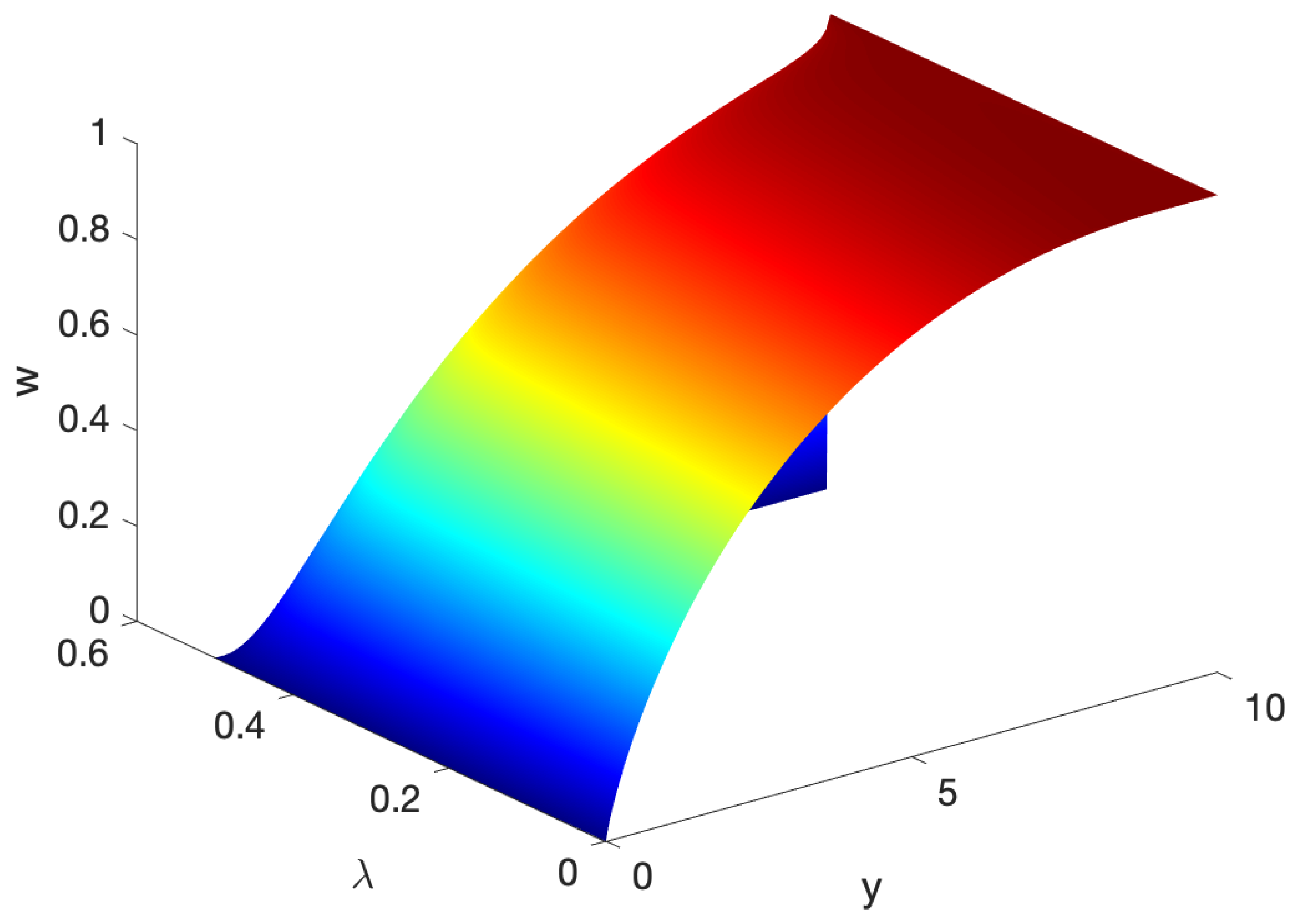
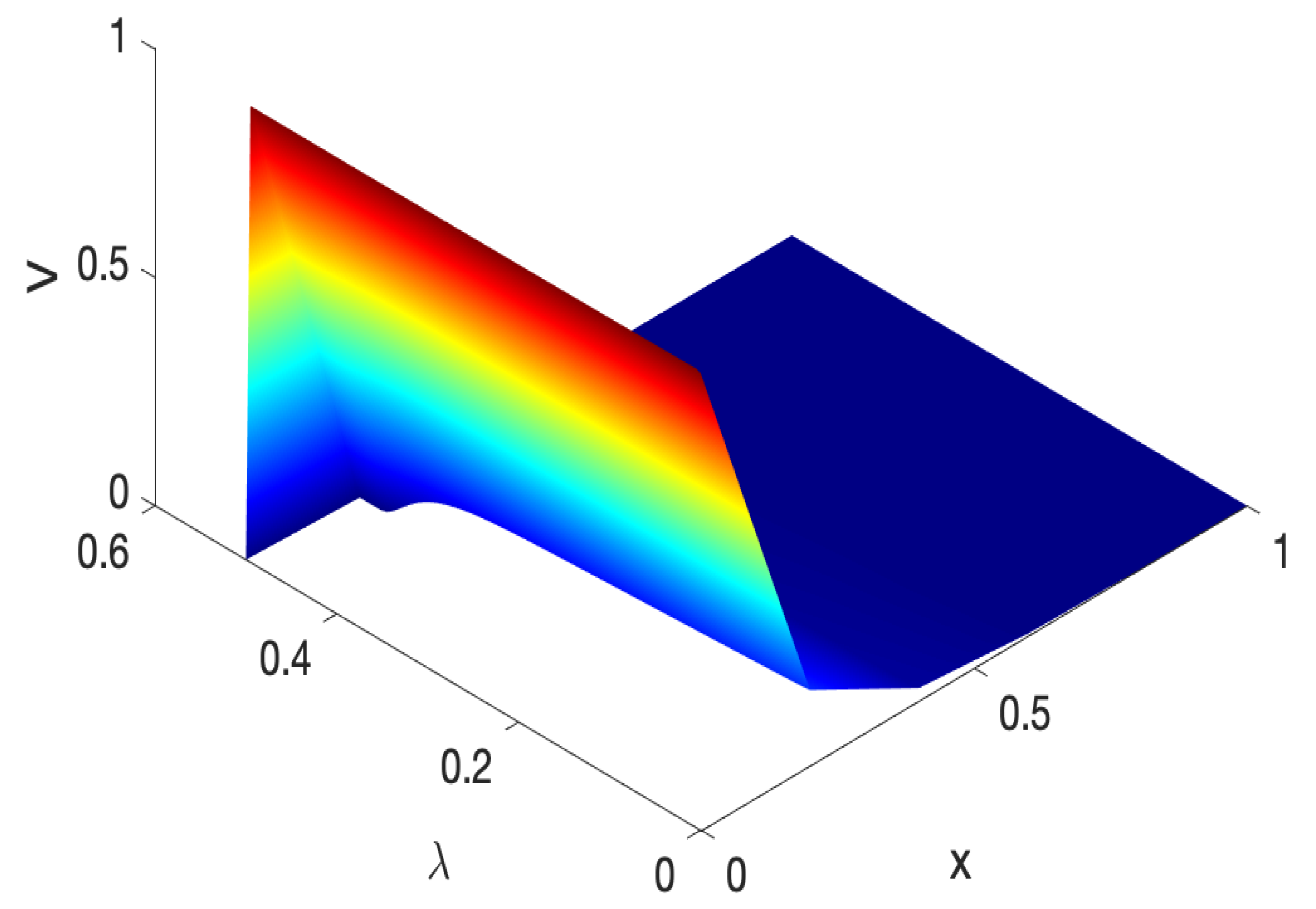
By using the parameters above, we plotted the dual value function. As we see in Figure 1, the dual value function is increasing and concave in the dual variable. We also see from Figure 2 that the value function is decreasing and convex in the initial wealth.

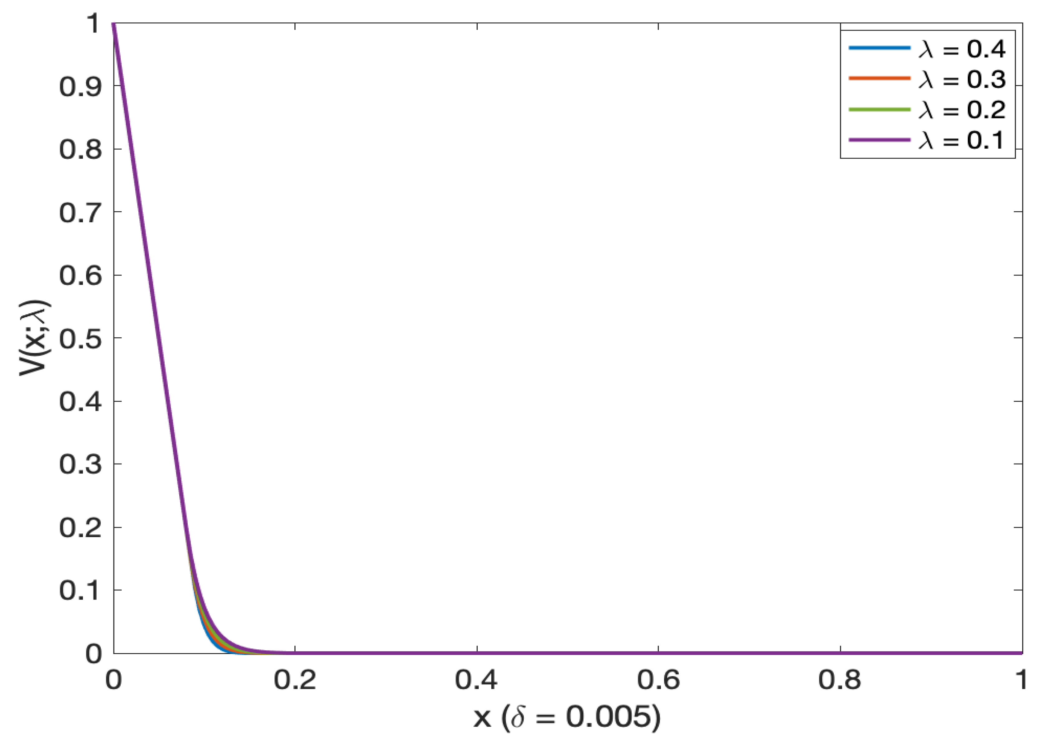
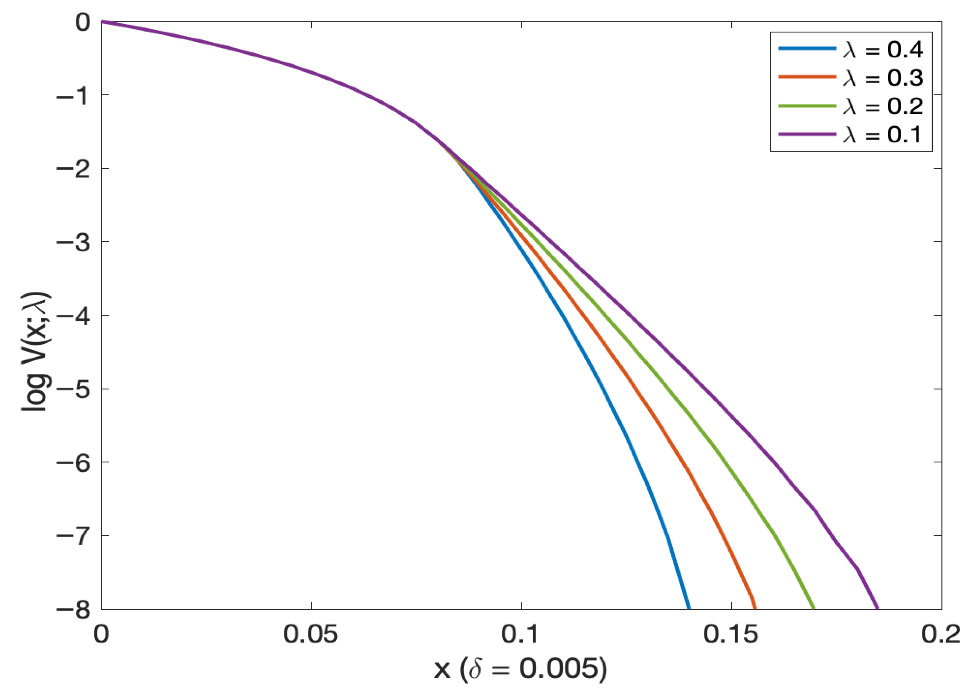
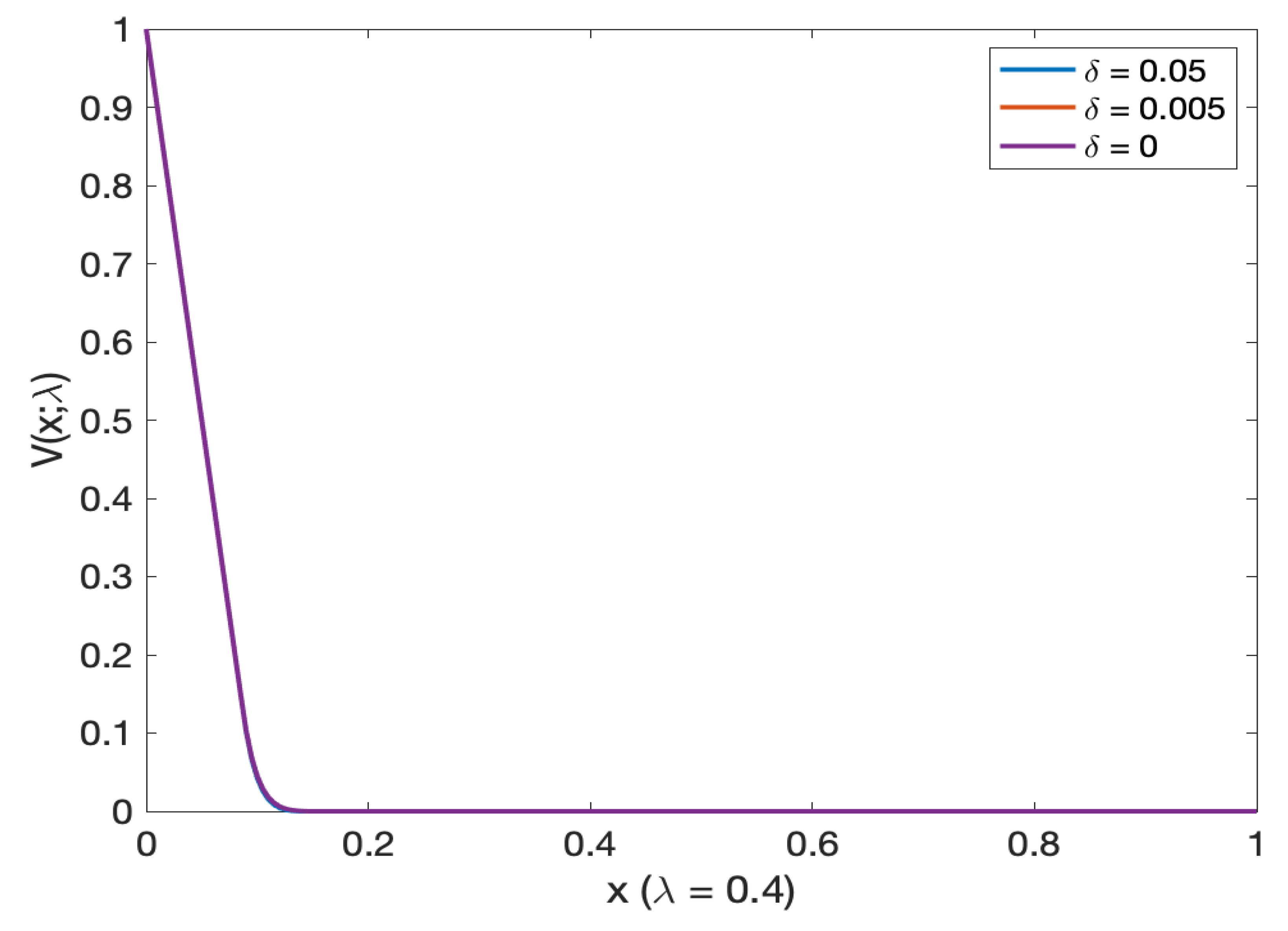
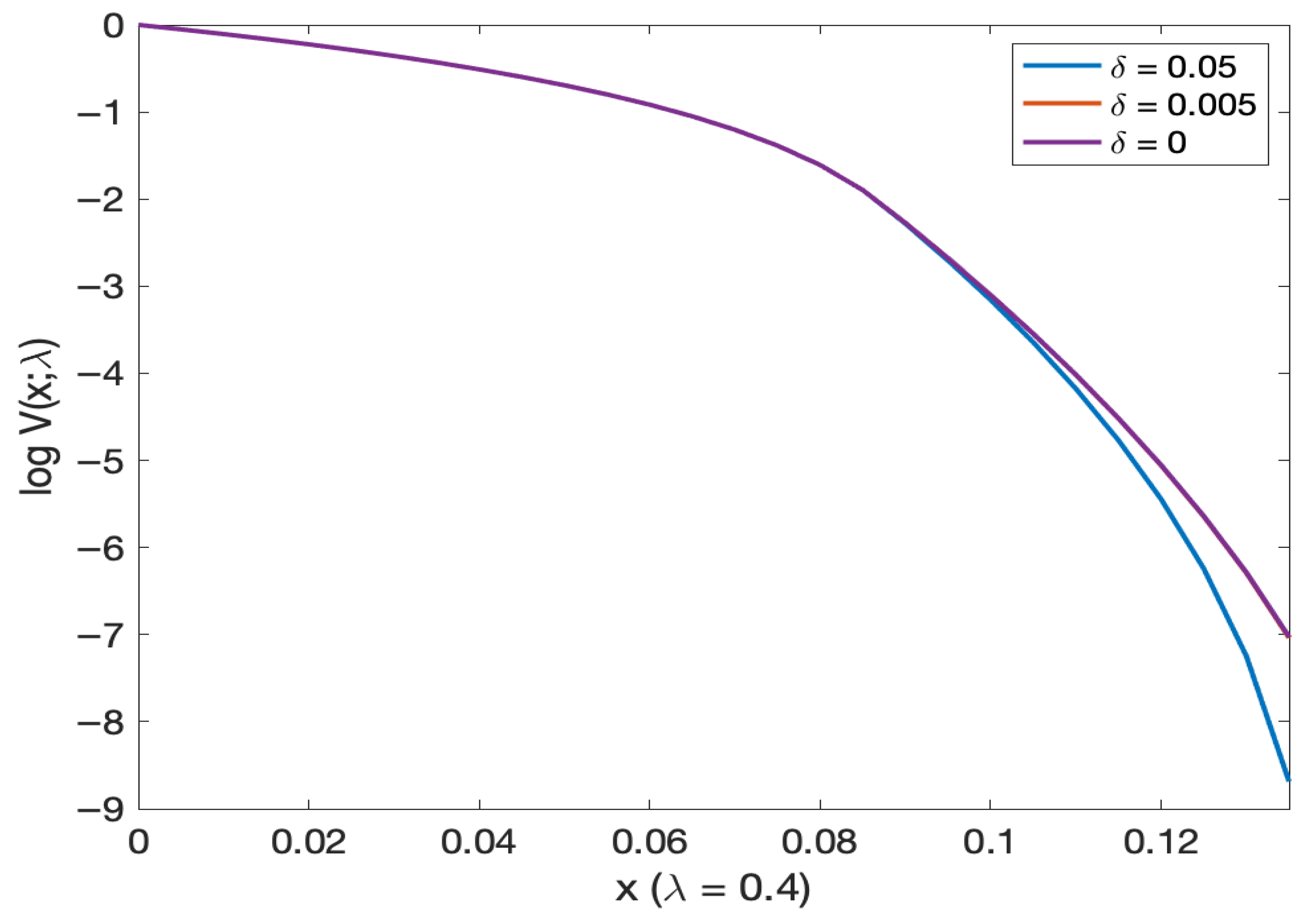
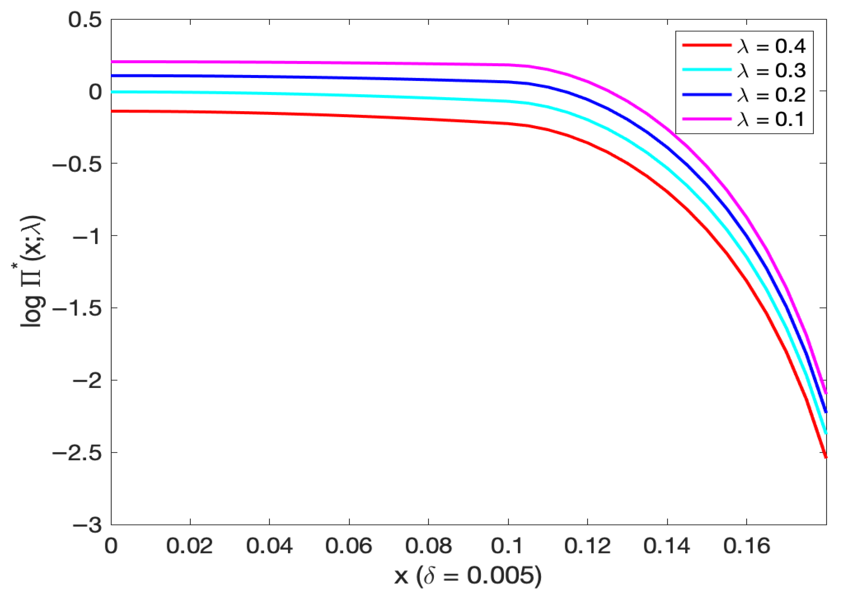
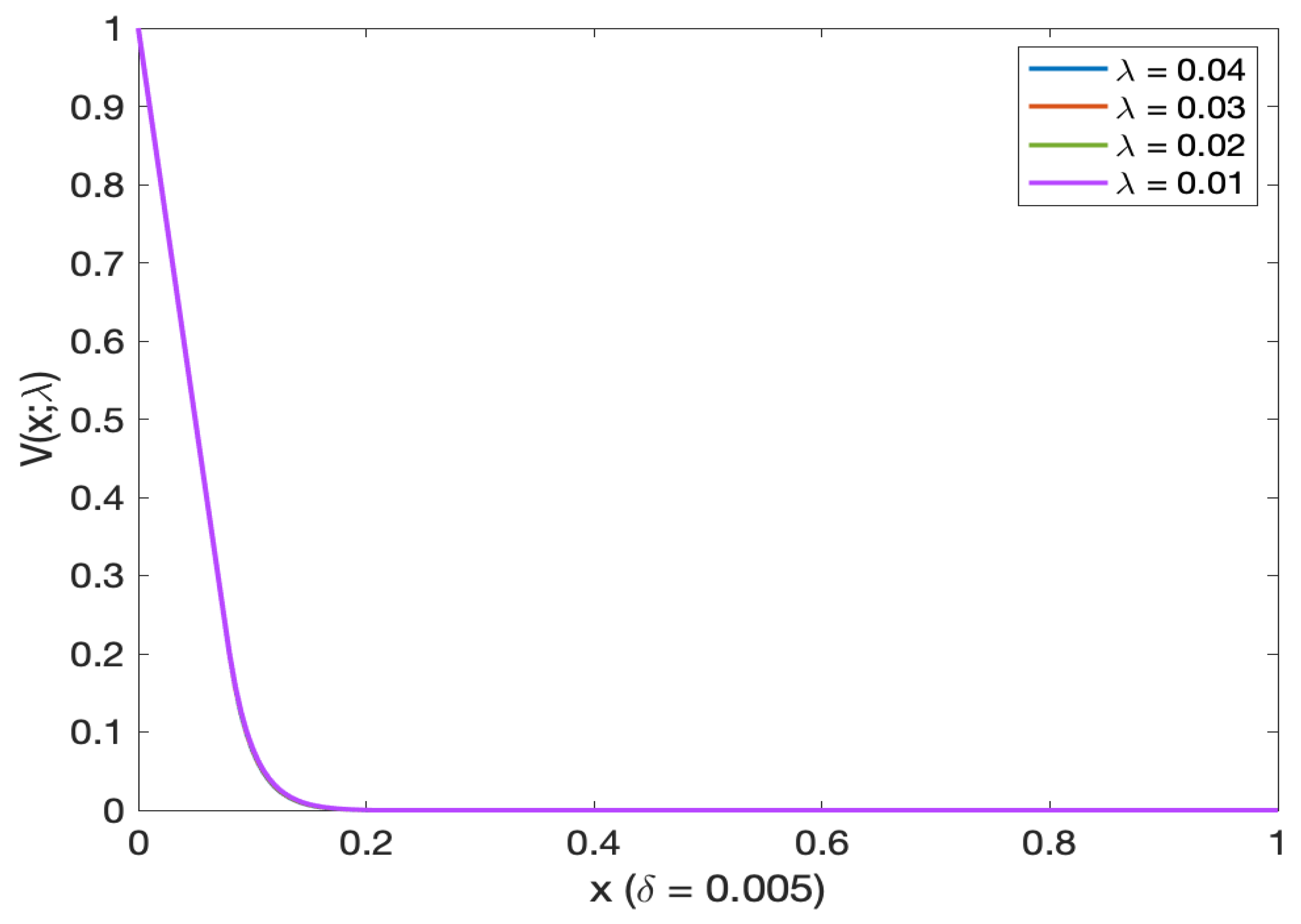
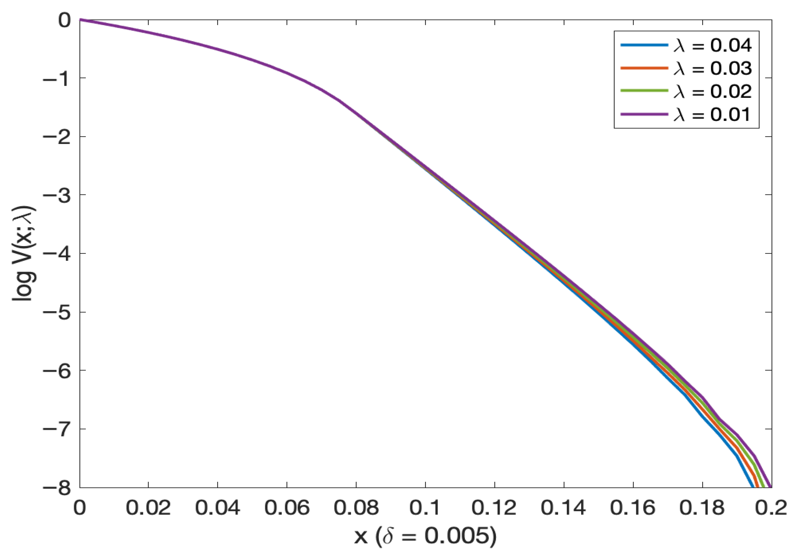
Figure 3 (log probability of default in Figure 4) and Figure 5 (log probability of default in Figure 6) illustrated the probability of default (and, respectively, log probability of default in Figures as a function of initial wealth for different mortality intensity levels). We see that the probability of default decreases as we increase the initial wealth (this is true for all different initial mortality intensities). This probability approaches 0 as the initial wealth exceeds 0.15. From Figure 5 (and Figure 6) we see that the probability of default is almost the same for very small levels of initial mortality intensity. 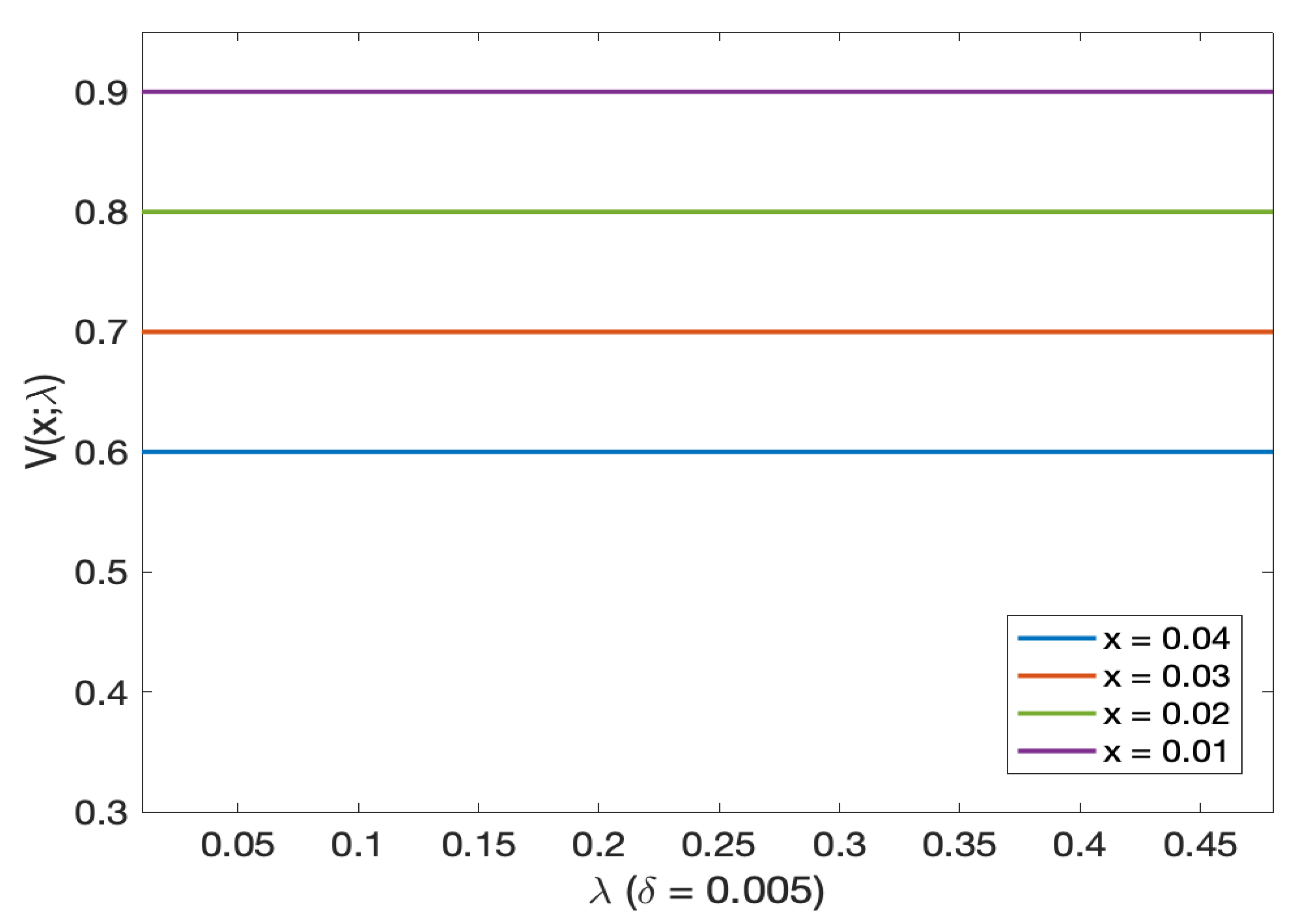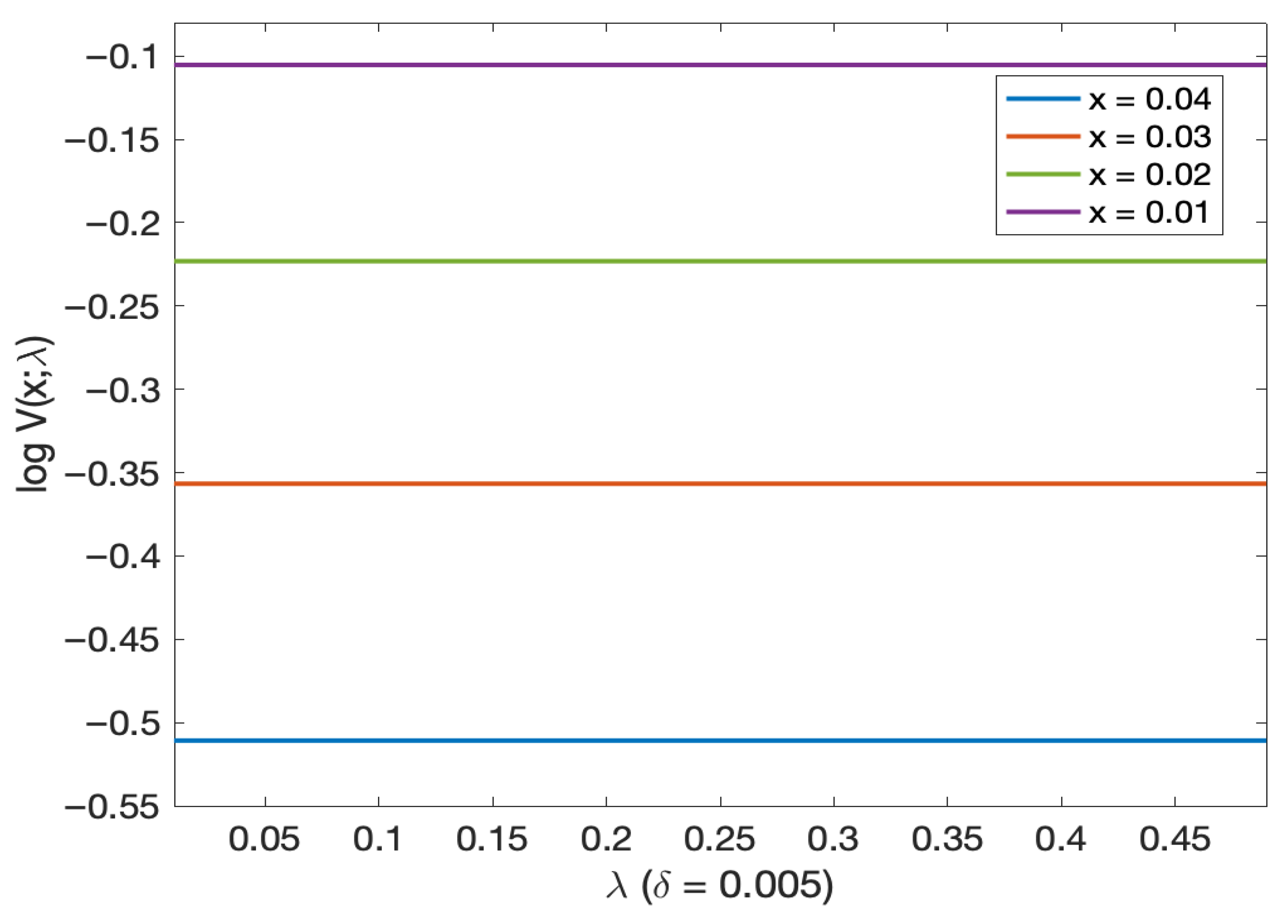From Figure 7 (and Figure 8 on log scale) for very small initial wealth levels, the probability of default does not change with mortality intensity.

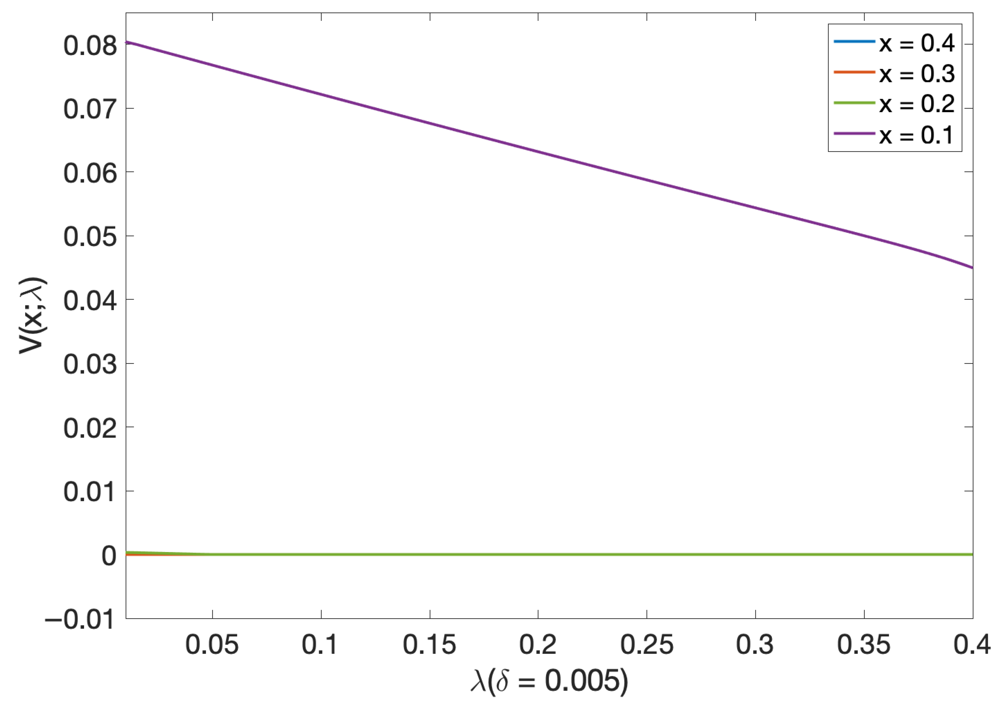
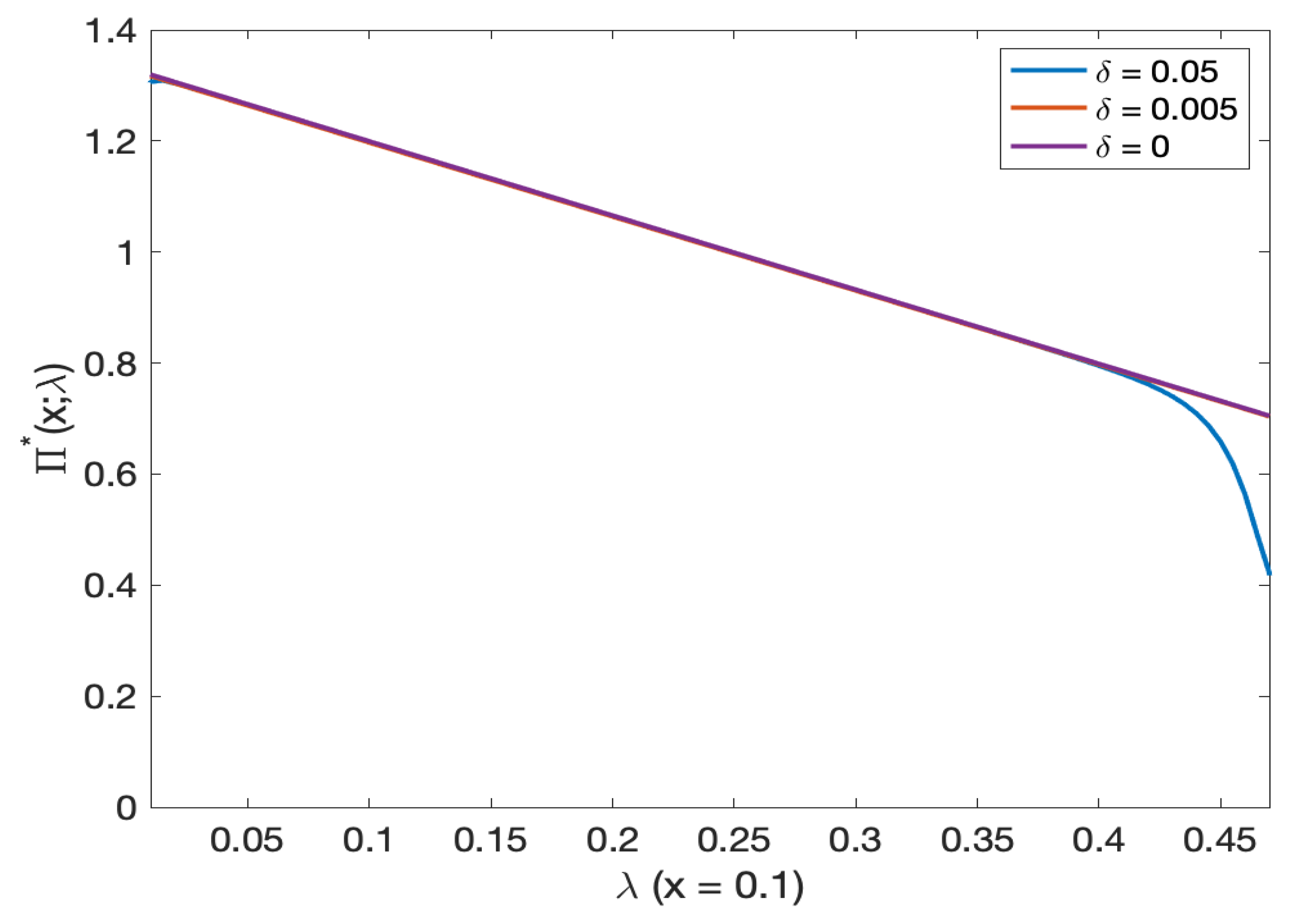
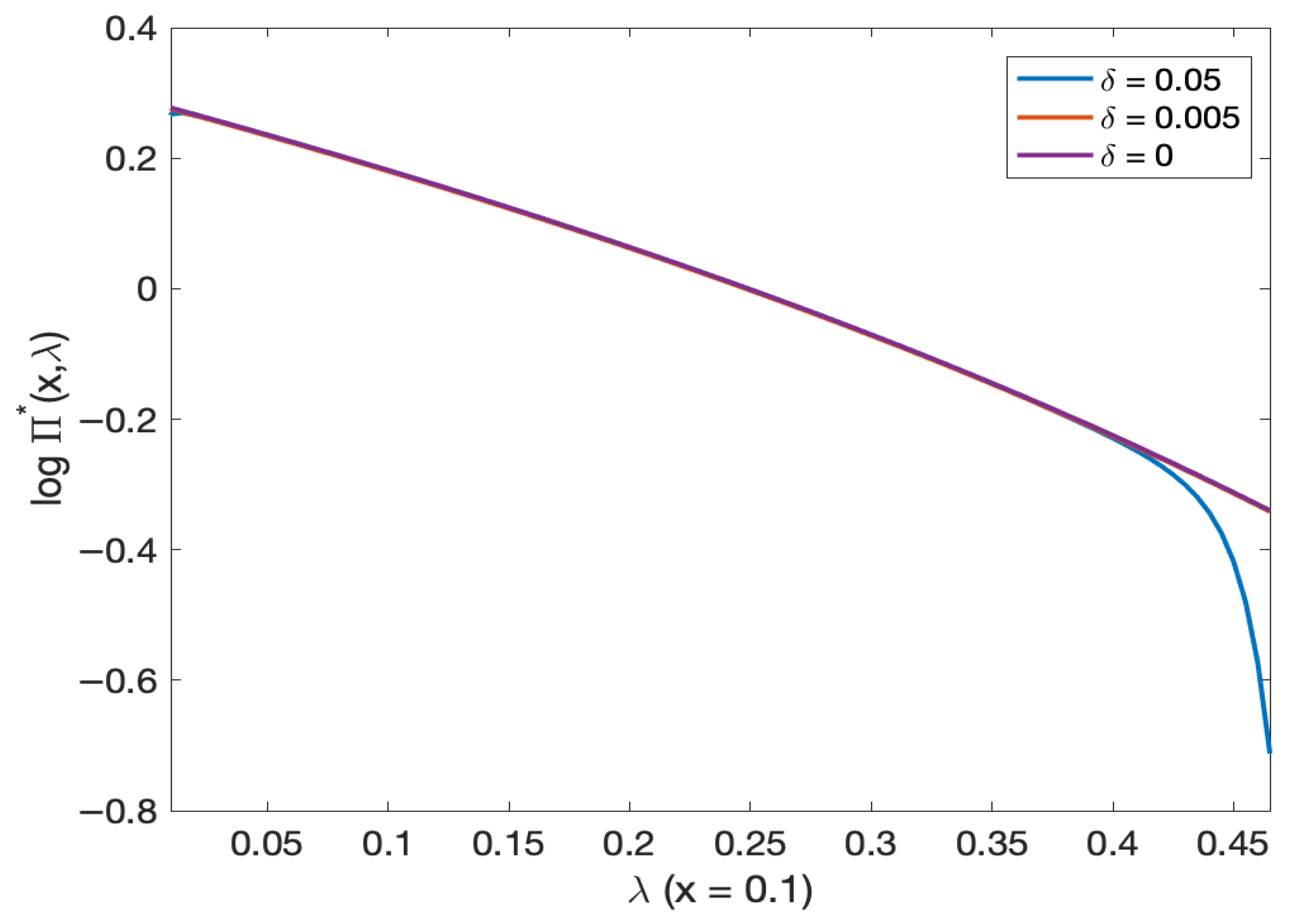
Additionally, we see from Figure 9 that the probability of default decreases as the mortality intensity increases, as expected. Suppose the initial mortality intensity is higher than 0.1. The probability of default is very close to zero. In addition, the curves corresponding to $x=0.2$, $x=0.3$, and $x=0.4$ are identical to zero.

We notice that the probability of default is lower in stochastic intensity models and this effect is more pronounced if the volatility of mortality intensity is increased. Let us provide a theoretical justification for this result; for this, consider two models for the stochastic intensity

$$d{\lambda }_i(t)=A{\lambda }_i(t)dt+{\delta }_i\sqrt{{\lambda }_i(t)}dB(t),i=1,2,$$

with ${\delta }_2>{\delta }_1.$ Then, by Theorem 4.1 in Hajek (1985), ${\lambda }_2(t)$ dominates ${\lambda }_1(t)$ in the following sense

$$E[\Phi ({\lambda }_2(t))]\ge E[\Phi ({\lambda }_1(t))],$$

for every convex nondecreasing function $\Phi .$ The lower probability of default is then explained by a higher expected drift ${\lambda }_2(t)Y(t)$ in Equation (2).

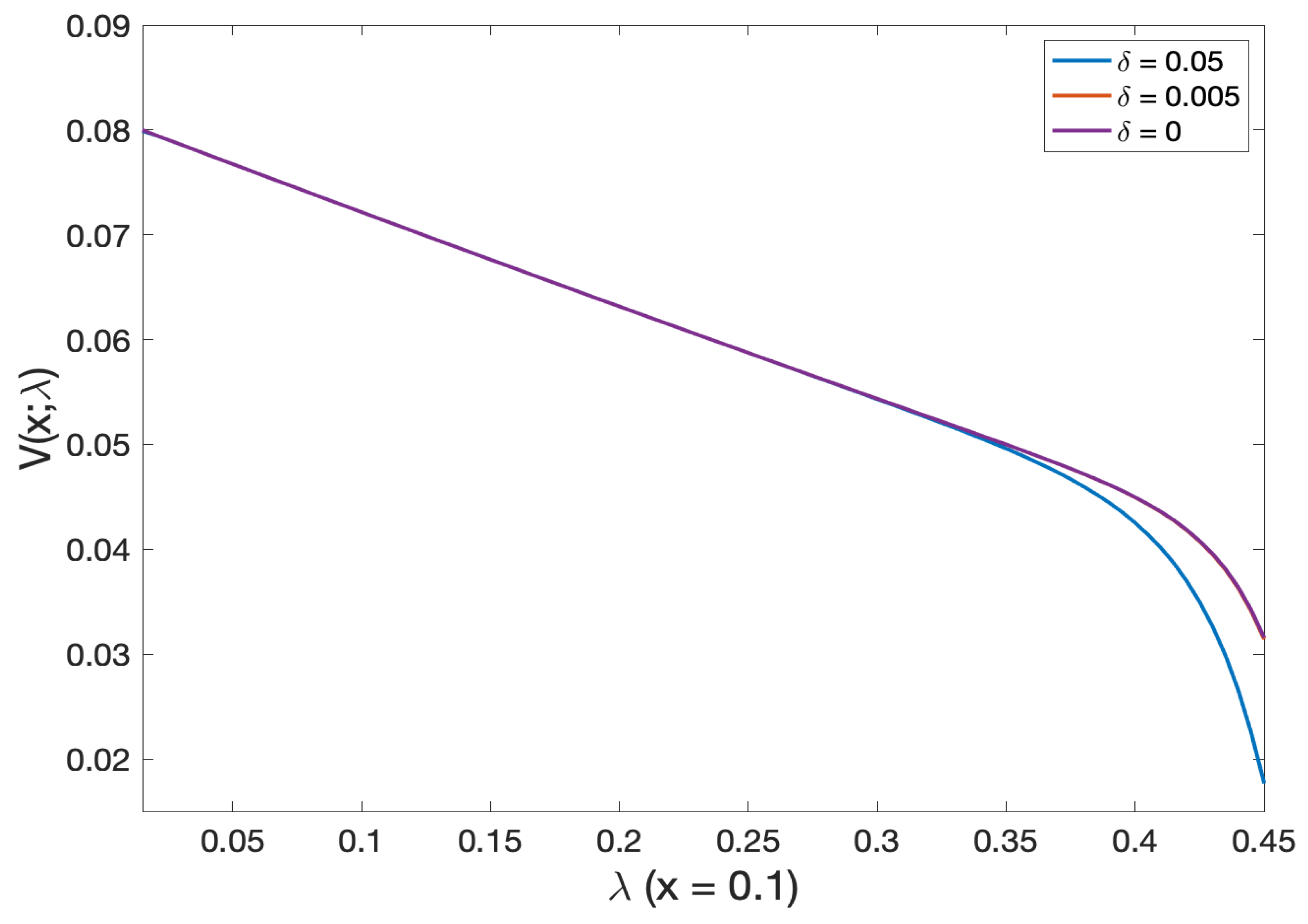
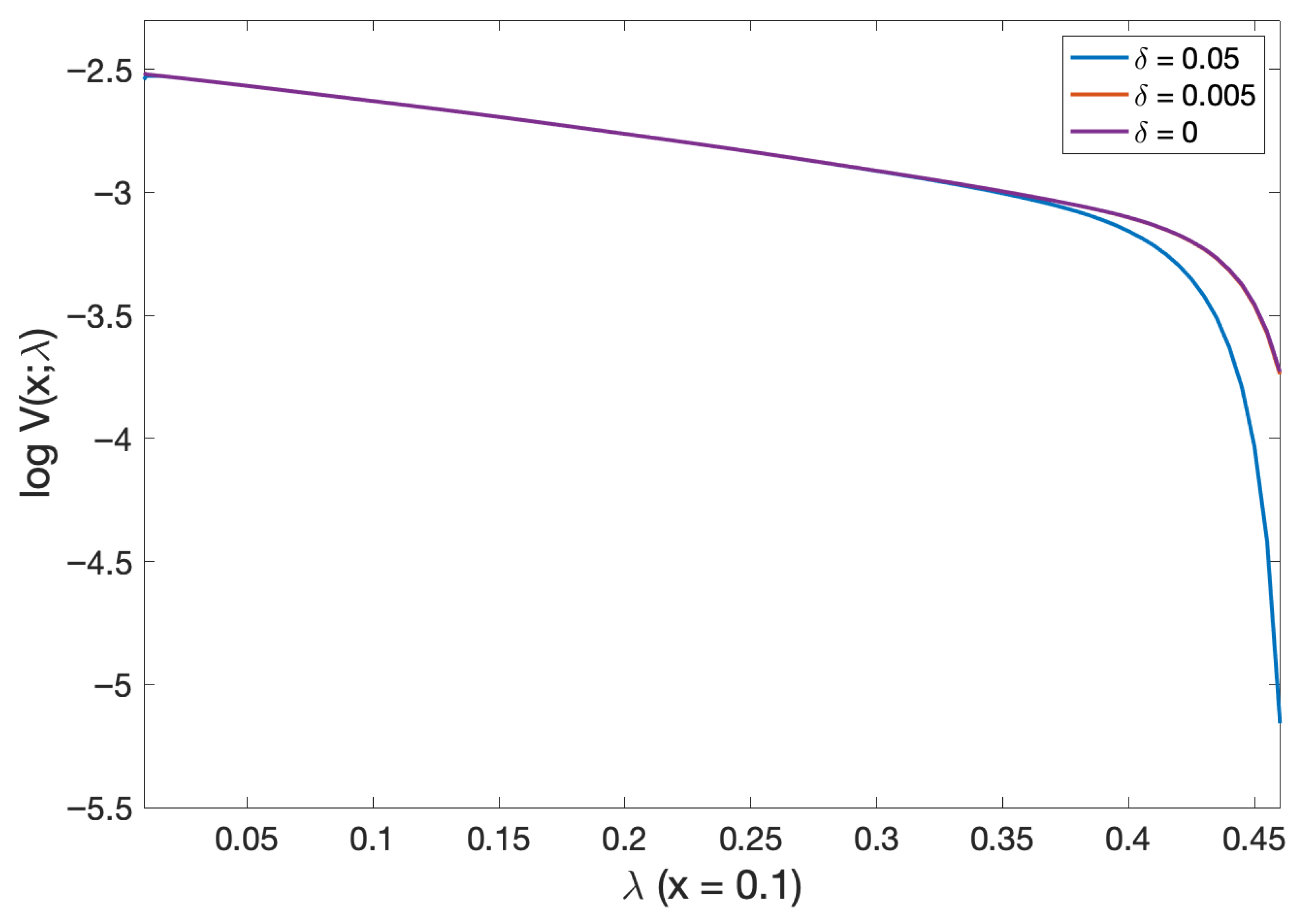
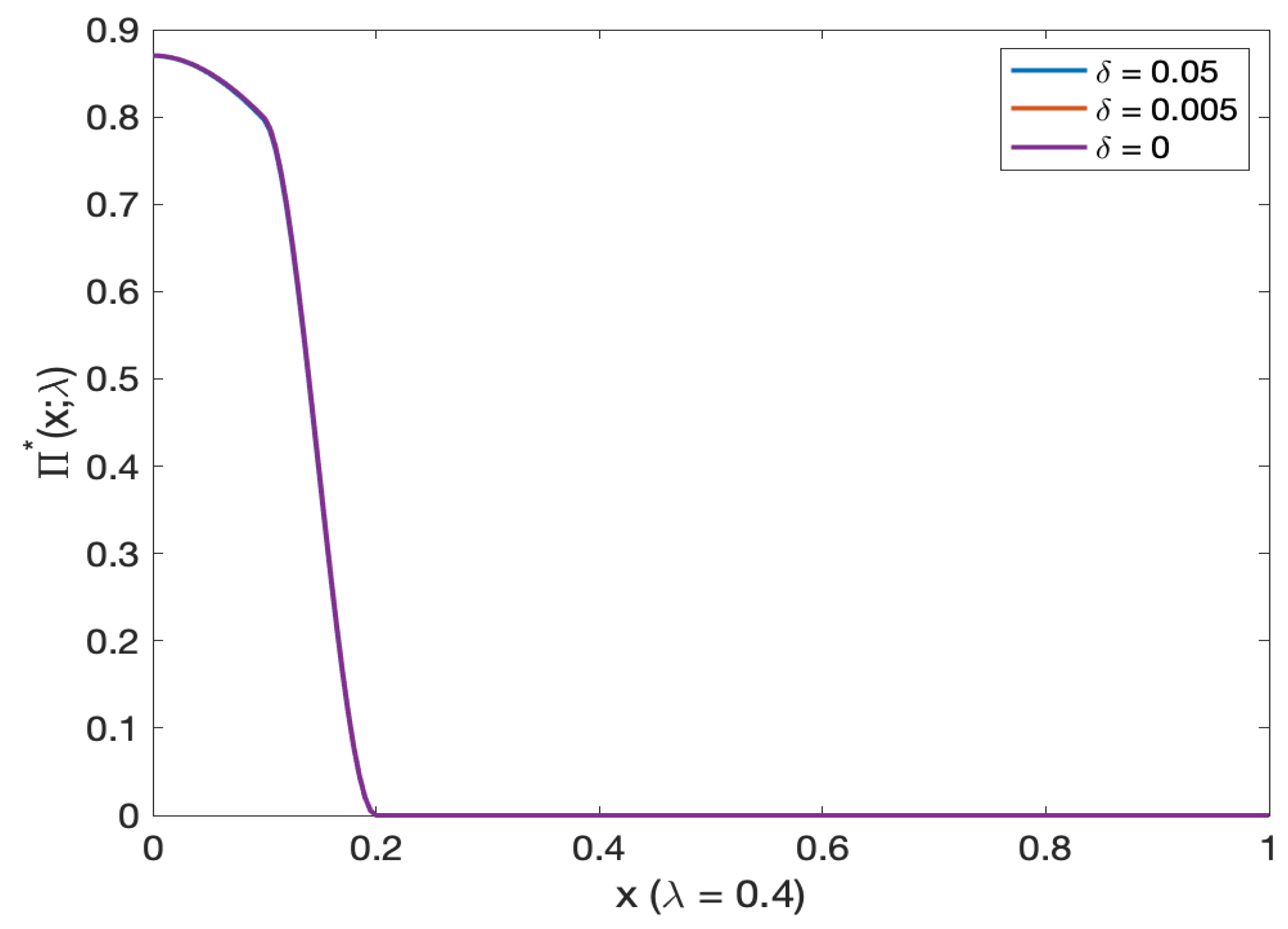
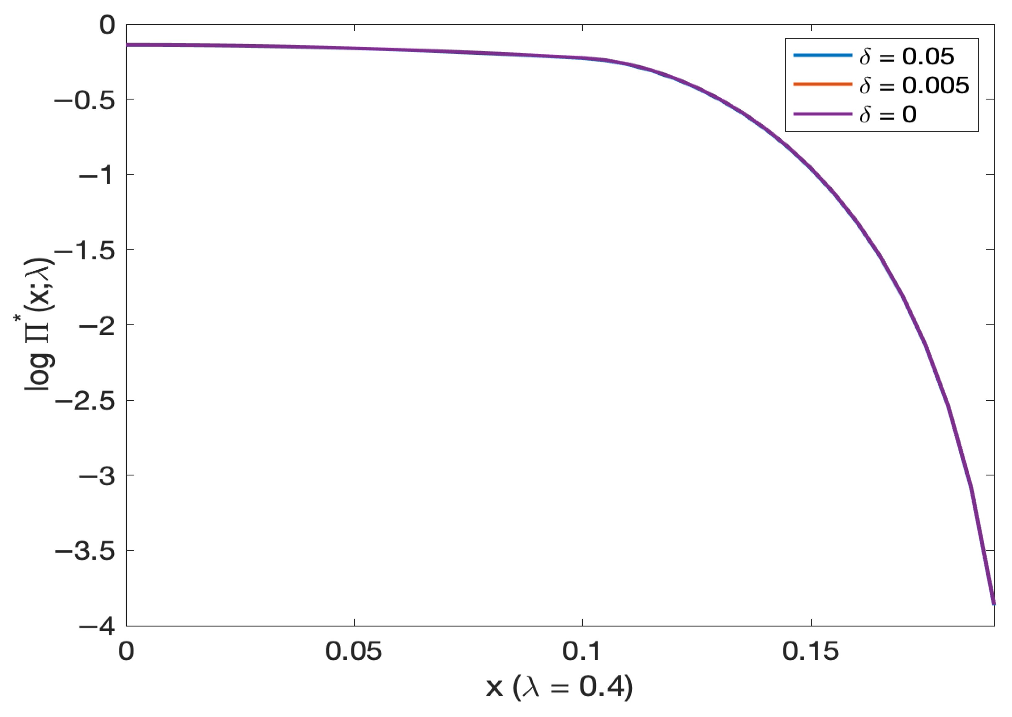
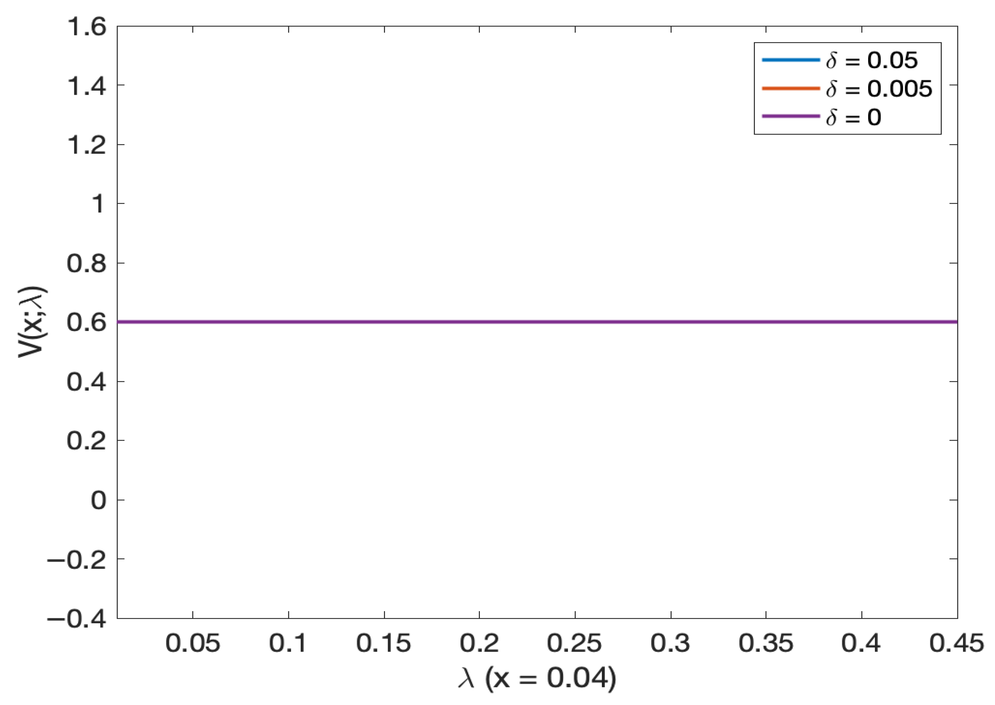
We see from Figure 10 that the probability of default (or log probability of default in Figure 11) is more negligible for the higher volatility of the stochastic mortality intensity (see Lemma 2 for an intuition of this result). Meanwhile, from Figure 12, we found that for very small initial wealth, the probability of default is the same for all different values of volatility intensity. Then from Figure 13 the probability of default (and, log probability of default in Figure 14) shares is approximately the same for varying volatility of stochastic models. Moreover, we see that the probability of default decreases as we increase the initial wealth and gets very close to zero.

5.2. The Investment Strategy

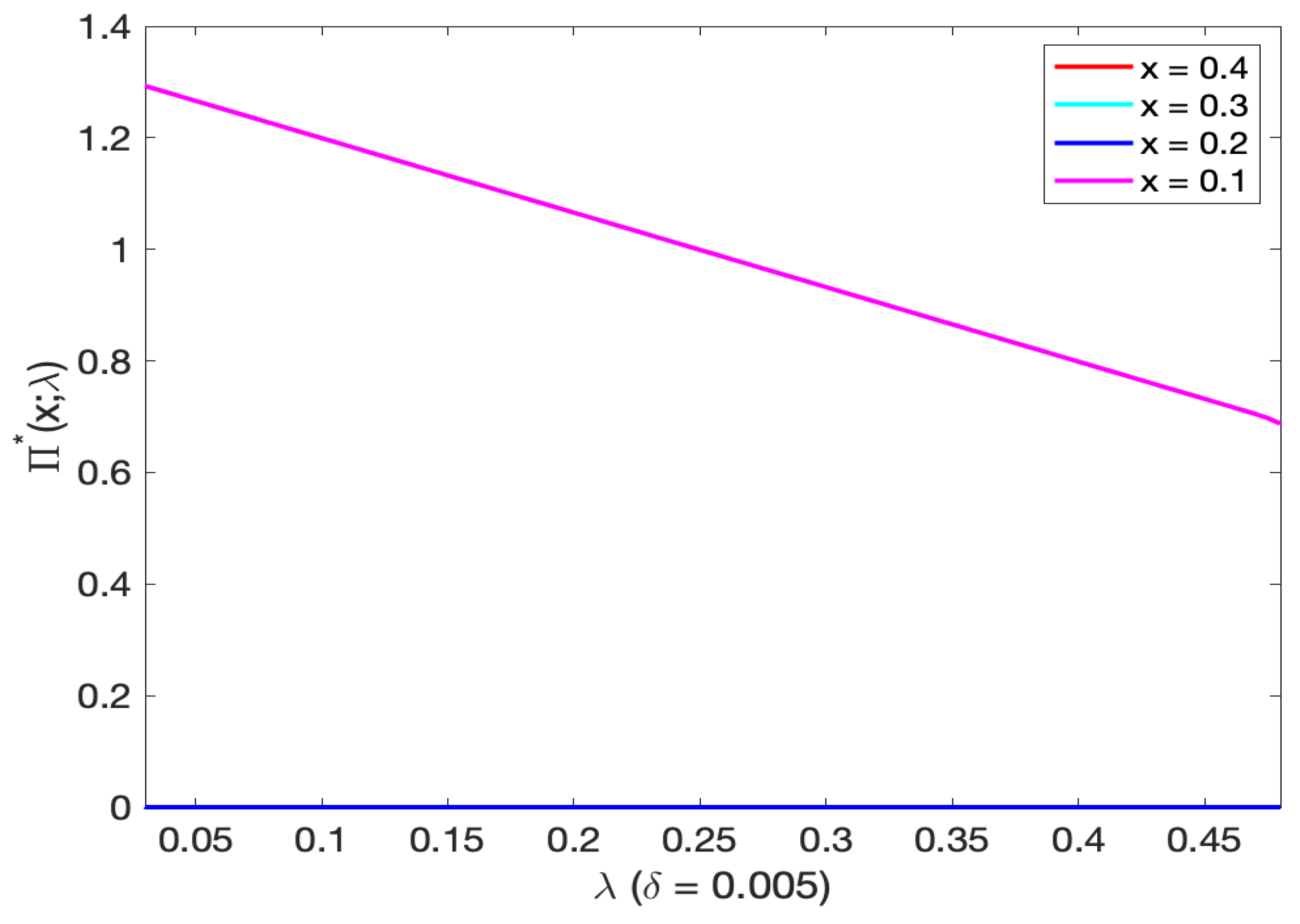
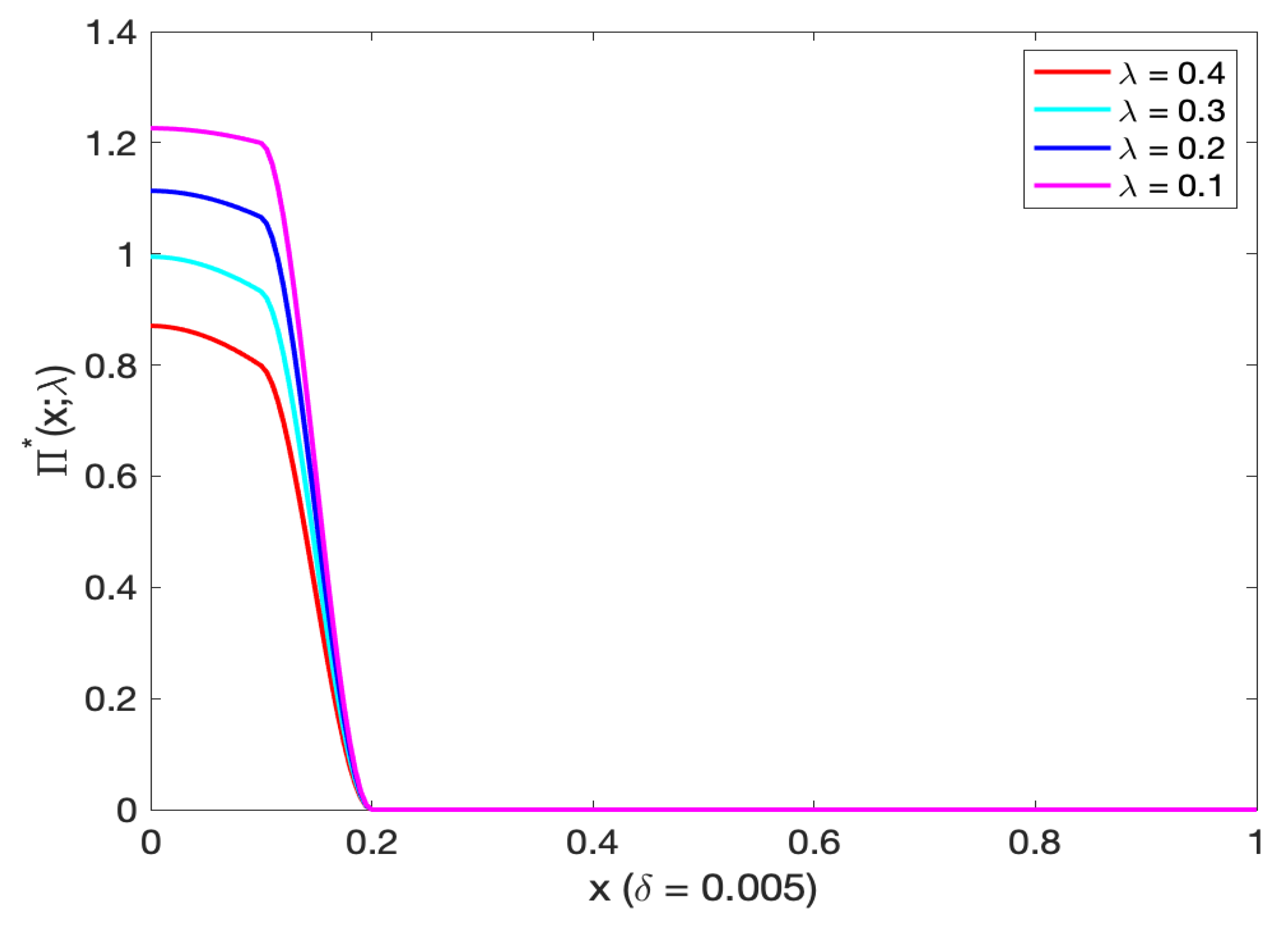
From Figure 15, we see that the optimal investment decreases as the mortality intensity increases. The optimal investment is nearly zero if the initial wealth is higher than 0.1. When $x=0.3$ and $x=0.4$, the curves of the optimal investment are zero. From Figure 16 (and Figure 17 on log scale) we found that the optimal investment decreases as both the initial wealth and mortality intensity increase. The optimal investment approaches zero after exceeding 0.19.

5.2.1. Comparison with Deterministic Intensity Model

For varying volatility of stochastic models, the optimal investment decreases by increasing the initial mortality intensity (see Figure 18 and on a log scale Figure 19). In addition, the optimal investment for $\delta =0.05$ is slightly lower than other stochastic model volatility. The amount invested in the stock decreases with the initial wealth (see Figure 20 and Figure 21).

5.2.2. Dependence on Sharpe Ratio

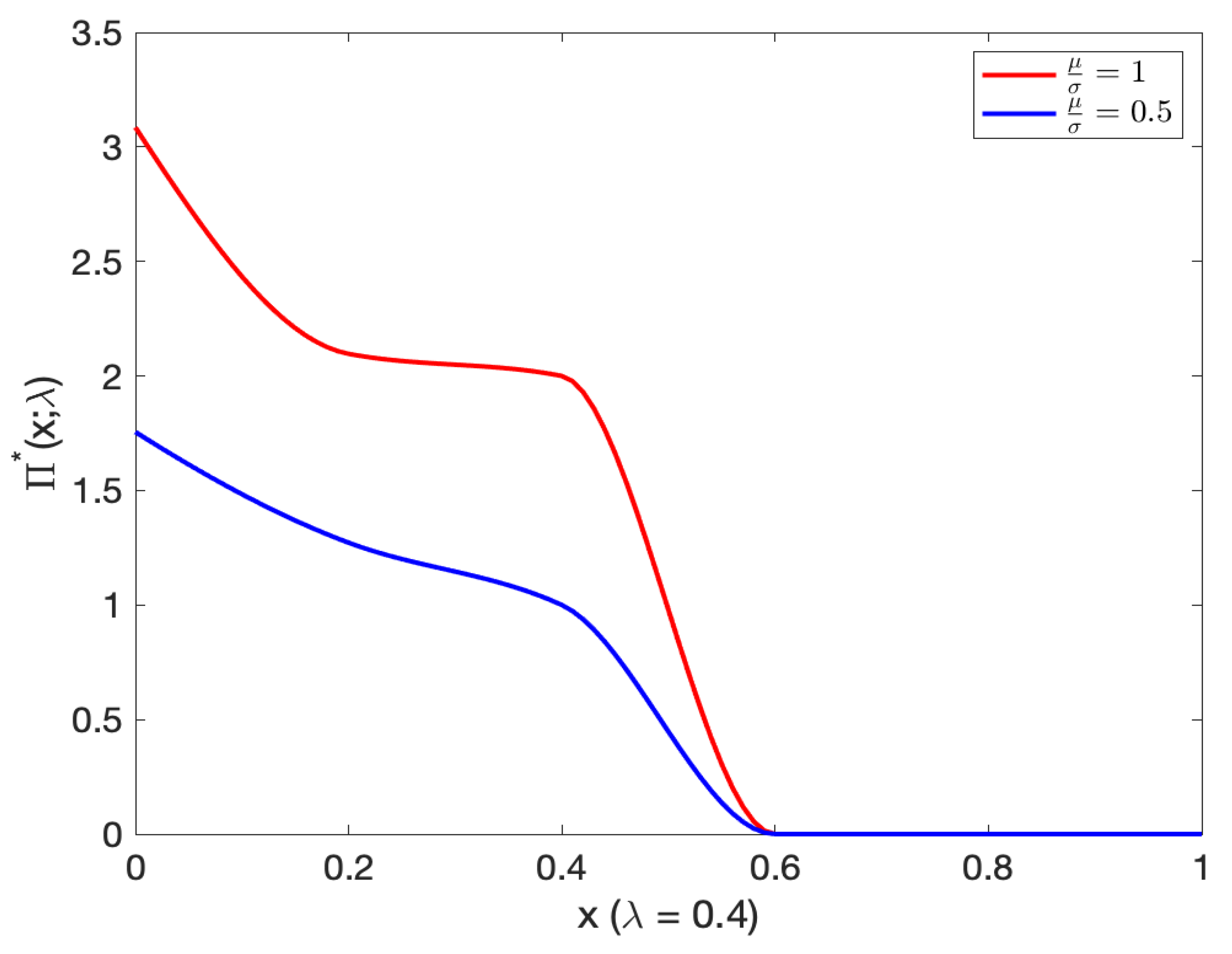
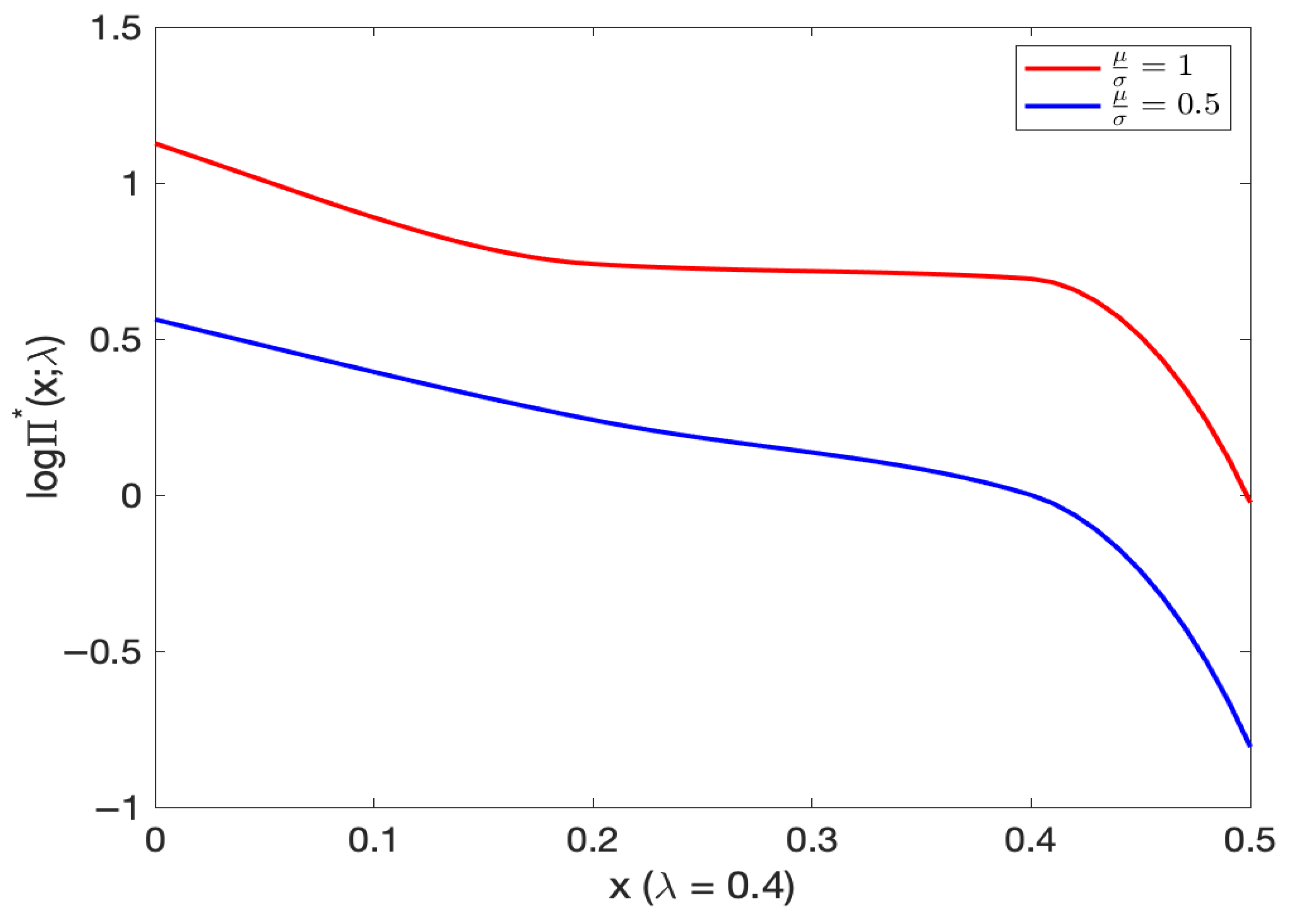
The optimal investment decreases as initial wealth increases for varying Sharpe ratios, ${\displaystyle \frac{\mu }{\sigma }}$ (See Figure 22 and Figure 23). Moreover, the optimal investment with ${\displaystyle \frac{\mu }{\sigma }}=1$ ($\mu =0.05$, $\sigma =0.05$) was slightly higher compared with ${\displaystyle \frac{\mu }{\sigma }}=0.5$ ($\mu =0.025$, $\sigma =0.05$).

5.3. Interpretation in Terms of Reserves and Capital Requirements

In our work, the value function $V(x,\lambda )$ represents the probability that a life insurance company with initial wealth x and current mortality intensity $\lambda$ defaults (ruins) before the random termination time ${\tau }_d$. In actuarial terms, $V(x,\lambda )$ thus links an insurer’s capital position to its probability of default. It therefore provides the key ingredient needed to determine risk-based reserves, i.e., the level of assets required to guarantee that the company remains solvent with a prescribed probability.

Regulatory and internal solvency frameworks (e.g., Solvency II or RBC in the U.S.) specify a target level of tolerable default probability $p^{\star }$, typically between $0.5\%$ and $1\%$ over the planning horizon. Given this safety level, the minimal initial wealth that achieves it under our model conditions is defined as the required reserve

$$R(\lambda )=inf\{x\ge 0:V(x,\lambda )\le p^{\star }\}.$$

(15)

Because $V(x,\lambda )$ is continuous and strictly decreasing in x (as shown in our numerical results), there exists a unique solution to (15) for each $\lambda >0$. Thus, the value function $V(x,\lambda )$ computed from the dual PDE, in a purely numerical procedure, can be directly inverted along the x-axis to obtain the reserve function $R(\lambda )$ for any desired tolerance $p^{\star }$.

Equation (15) thus establishes a one-to-one mapping between the level of available capital and the associated solvency probability. Higher initial wealth reduces the likelihood of default, while higher mortality intensity $\lambda$ (which corresponds to shorter expected lifetime of the insured population) also decreases the probability of default because future annuity obligations become smaller in expectation. Hence, a mortality improvement (lower $\lambda$) requires higher reserves, whereas greater mortality volatility increases capital needs due to higher uncertainty about future liabilities. Our numerical results confirm these qualitative patterns.

The comparative analysis between deterministic and stochastic mortality models reveals that introducing CIR stochastic mortality reduces $V(x,\lambda )$ across the entire domain of x, indicating lower default probabilities for the same initial wealth. Consequently, the reserve required to achieve a fixed solvency target $p^{\star }$ is lower under stochastic mortality than under deterministic assumptions. This implies reduction in required reserves purely due to the more realistic stochastic representation of longevity dynamics. Ignoring mortality stochasticity can therefore lead to overly conservative reserve estimates and inefficient capital allocation.

6. Conclusions and Future Work

We conclude by summarizing the main findings, outlining the main contributions of this work, and elucidating directions for future research.

First, the probability of default decreases with both initial wealth and initial mortality intensity. This relationship also holds for different volatilities of stochastic intensity. The volatility of stochastic intensity has little effect on the probability of default; however, higher volatility yields slightly lower default probabilities. Higher values of stochastic mortality intensity also result in marginally lower default risk, while for very small initial mortality intensities, the probability of default remains essentially unchanged.

Thus, in the more realistic stochastic intensity model developed in this paper, we obtain the opposite result relative to the constant or Brownian mortality assumptions in Cahyaningtias et al. (2023): the probability of default is lower in stochastic intensity models, and this effect becomes more pronounced as the volatility of mortality intensity increases. Hence, compared to Cahyaningtias et al. (2023), the results show that incorporating a CIR-based stochastic mortality process provides new quantitative insights.

Second, the optimal amount invested in the stock is decreasing in the initial wealth and the initial mortality intensity; it is nearly constant for small values of initial wealth. The volatility of stochastic intensity has little effect on the optimal investment; for higher values of stochastic mortality intensity, we see slightly lower values for the optimal amounts invested in stock. We see higher values for the optimal amount invested in stock as Sharpe ratio gets larger.

Thus, in the context of a realistic mortality intensity model, the insight of decreasing pattern of the optimal allocation to the risky asset with respect to wealth and mortality intensity represents the paper’s main economic insight. It formalizes a prudential, solvency-preserving behavior that arises endogenously from the optimization framework. When the insurer’s wealth (capital) increases, the marginal benefit of taking additional market risk declines relative to the potential cost of default, leading to a reduction in risky investment. Likewise, when mortality intensity (liability risk) rises, the model prescribes a more conservative portfolio to preserve liquidity and solvency.

This behavior is consistent with the risk-sensitive principles underlying Solvency II and risk-based capital (RBC) regimes. Specifically, our model derives from first principles why prudent insurers would endogenously reduce risky asset allocation as capital increases or liability risk rises. The model thus provides a theoretical foundation for understanding the economic rationale behind capital-sensitive investment behavior.

From a technical perspective, the computed value function $V(x,\lambda )$ not only determines the optimal investment policy but also yields an operational measure of capital adequacy. The reserve function $R(\lambda )$ derived from $V(x,\lambda )=p^{\star }$ can be viewed as the insurer’s state-dependent solvency threshold. Our findings imply that (i) reserves decrease with mortality deterioration (higher $\lambda$), (ii) reserves increase with volatility of mortality intensity, and (iii) stochastic mortality models lead to smaller, yet more accurate, reserve estimates than deterministic approaches. This interpretation establishes a clear practical link between the theoretical optimization framework and real-world solvency management under longevity uncertainty.

In addition, the model serves as a quantitative tool for evaluating the appropriate level of risky investment given an insurer’s solvency position or liability structure. It enables stress testing of default probabilities and optimal allocations under regulatory-like scenarios such as mortality shocks, capital erosion, or market downturns. Finally, it establishes a basis for future extensions, such as multi-cohort portfolios, to assess diversification and longevity-hedging effects within solvency capital modeling.

Specifically, starting from De Rosa et al. (2021), one may extend the framework first to two cohorts, with mortality modeled through their respective stochastic intensities as

$$d{\lambda }_i(t)=A_i{\lambda }_i(t)dt+{\delta }_i\sqrt{{\lambda }_i(t)}d{B}_i(t),i=1,2,$$

for some positive parameters $A_i$ and ${\delta }_i$, $i=1,2$. Here $B_1$ and $B_2$ denote independent Brownian motions, though the model can easily be generalized to allow for correlated Brownian motions.

Our setting naturally admits a straightforward extension to multiple cohorts. Let $I_i(t)$ denote the proportion of individuals in cohort i who are alive at time t,

$$I_i(t)=exp\left(-{\int }_0^t{\lambda }_i(u)du\right),i=1,2.$$

Under this two-cohort structure, the wealth dynamics of the insurer are given by

$$dX(t)=\pi (t)X(t)(\mu dt+\sigma dW(t))-K_1{e}^{-{\int }_0^t{\lambda }_1(u)du}dt-K_2{e}^{-{\int }_0^t{\lambda }_2(u)du}dt,X(0)=x,$$

where, as before, $\pi (t)$ denotes the proportion of wealth invested in the stock at time t.

Let ${\tau }_d$ represent the random time at which the company ceases operations, assumed to be exponentially distributed with intensity $\gamma$, and define the bankruptcy time

$${\tau }_0:=inf\{t\ge 0:X(t)=0\}.$$

The insurer’s optimization problem is then to minimize the probability of default before cessation:

$$V(x,{\lambda }_1,{\lambda }_2)=\underset{\pi }{inf}\mathbb{P}\left[{\tau }_0\le {\tau }_d|X(0)=x,{\lambda }_1(0)={\lambda }_1,{\lambda }_2(0)={\lambda }_2\right].$$

The associated value function satisfies a Hamilton–Jacobi–Bellman (HJB) equation. The analytical challenge arises because the value function depends on the cumulative mortality intensity processes ${\Lambda }_i(t)={\int }_0^t{\lambda }_i(u)du$, $i=1,2$, which increases the effective dimensionality by three relative to the single-cohort case. Consequently, the dual value function also satisfies a higher-dimensional partial differential equation. Thus, developing a numerically stable and convergent scheme for solving this PDE represents an important direction for future research.