Abstract
Phytoremediation is an eco-friendly and in situ solution for remediating heavy metal-contaminated soils, yet practical application requires timely and accurate effectiveness evaluation. However, conventional chemical analysis of plant parts and soils is labor-intensive, time-consuming and limited for large-scale monitoring. This study proposed a rapid sensing framework integrating laser-induced breakdown spectroscopy (LIBS) with deep transfer learning and spectral indices to assess phytoremediation effectiveness of Sedum alfredii (a Cd/Zn co-hyperaccumulator). LIBS spectra were collected from plant tissues and diverse soil matrices. To overcome strong matrix effects, fine-tuned convolutional neural networks were developed for simultaneous multi-matrix quantification, achieving high-accuracy prediction for Cd and Zn (R2test > 0.99). These predicted concentrations enabled calculating conventional phytoremediation indicators like bioconcentration factor (BCF), translocation factor (TF), plant effective number (PEN), and removal efficiency (RE), yielding recovery rates near 100% for TF and PEN. Additionally, novel spectral indices (SIs)—directly derived from characteristic wavelength combinations—were constructed to bypass intermediate quantification. SIs significantly improved the direct evaluation of Zn removal and translocation. Finally, a decision-level fusion strategy combining concentration predictions and SIs enhanced Cd removal assessment accuracy. This study validates LIBS combined with intelligent algorithms as a rapid sensor tool for monitoring phytoremediation performance, facilitating sustainable environmental management.
1. Introduction
Soil contamination by heavy metals poses significant threats to ecological security and sustainable development, making its remediation a pressing global challenge [1]. Phytoremediation is an environmentally friendly and in situ remediation technology [2,3]. Hyperaccumulators, the plant species capable of accumulating large amounts of heavy metals, are the material basis of phytoremediation. Sedum alfredii, a well-known Cd/Zn co-hyperaccumulator [4,5], has gained widespread recognition for its high accumulation efficiency. It can be intercropped with crops, enabling simultaneous remediation and production, offering both economic and nutrient benefits [6,7,8,9]. These advantages highlight its value in promoting sustainable agricultural practices.
Accurate, timely, and systematic evaluation of phytoremediation is crucial for guiding scientific decision-making. Conventionally, the effectiveness of phytoremediation is assessed using indicators derived from the ratio between element concentrations in plant parts and soils [10,11]. Indicators like bioconcentration factor (BCF), translocation factor (TF), plant effective number (PEN), and removal efficiency (RE) are commonly used to assess heavy metal uptake, translocation, accumulation, and removal from the soil [10,11,12,13,14,15,16,17]. However, such evaluations entirely rely on chemical analysis of heavy metal concentrations, which requires complex, labor-intensive, and time-consuming pretreatment. Determining the heavy metal concentration of a single dried sample typically involves grinding, precise weighing, acid digestion, acid removal, volume adjustment, and instrumental quantification, taking over two hours to complete [18]. Given the spatial heterogeneity of heavy metal concentrations in soil [19], the need for numerous samples further increases the labor, time, and analytical costs, making these methods impractical for large-scale or low-budget remediation projects. Consequently, the entire process—from sampling to final evaluation—takes several days or weeks, delaying timely monitoring of phytoremediation and adjustment of remediation strategies [11].
Spectroscopic techniques offer an attractive advantage of rapid analysis and can efficiently acquire spectral data from a large number of samples. Spectral sensing-based monitoring of phytoremediation promises obvious benefits compared to traditional methods [20,21]. Existing studies on phytoremediation monitoring have focused on heavy metal determination by reflectance spectroscopy. For instance, visible and near-infrared (VNIR) spectroscopy was used to assess leaf spectral changes in heavy metal (Cd, Pb, and As) stressed plants [22,23]; VNIR hyperspectral imaging combined with deep learning was used to predict heavy metal concentrations in S. alfredii [24] and Miscanthus sacchariflorus [25]. However, reflectance spectroscopy relies on indirect correlations between spectral features and heavy metal concentrations, often resulting in limited quantitative accuracy.
Laser-induced breakdown spectroscopy (LIBS) is a powerful atomic emission-based technique that excels in elemental analysis [26]. It utilizes the pulsed laser to generate plasma on the sample surface, emitting characteristic spectral lines of constituent elements, enabling qualitative and quantitative detection [27]. LIBS stands out for rapid, remote, and multi-elemental analysis with minimal sample preparation, making it a promising tool for detecting heavy metals in plants and soils, particularly when integrated with intelligent learning algorithms [18,28]. For dried samples, the full detection process—including grinding, pellet pressing, spectral acquisition, and model prediction—can be completed within five minutes, offering a potential alternative for the rapid calculation of phytoremediation evaluation indicators [20].
To further enhance evaluation capability, spectral indices can be derived from LIBS data to capture metal-specific spectral characteristics through mathematically defined wavelength combinations. Similarly to the normalized difference vegetation index (NDVI) in remote sensing [29], such an index can simplify spectral data and improve correlation with phytoremediation indicators [20,30]. Incorporating spectral indices into LIBS-based evaluation can provide interpretable metrics and enable direct estimation of remediation performance, without requiring explicit metal concentration prediction. This approach simplifies model complexity and improves the efficiency of phytoremediation evaluation, providing timely support for monitoring and management decisions.
Despite the advantages of LIBS and artificial intelligence, their integration for systematic evaluation of phytoremediation effectiveness has rarely been explored. Previous studies have mainly focused on heavy metal quantification, while giving limited attention to the direct assessment of phytoremediation effectiveness. To bridge this gap, this study proposed an intelligent evaluation framework integrating LIBS with deep transfer learning and spectral indices for the rapid evaluation of phytoremediation effectiveness in the soil—S. alfredii system. The specific objectives are (1) to establish high-accuracy quantitative models for Cd and Zn detection in soil—S. alfredii system and derive phytoremediation indicators; (2) to construct spectral indices from sensitive spectral features of Cd and Zn for direct estimation of phytoremediation effectiveness; and (3) to integrate the evaluation results from concentration prediction and spectral index through decision-level fusion. Overall, this study extended the application of LIBS from elemental quantification to comprehensive phytoremediation assessment, providing a practical tool for evaluating and managing soil remediation effectiveness.
2. Materials and Methods
2.1. Plant Cultivation and Heavy Metal Treatment
The hyperaccumulating ecotype of S. alfredii was originally collected from an ancient mine in Quzhou, Zhejiang Province, China. Parent plants were cultivated in uncontaminated soil for at least three generations to minimize internal heavy metal concentrations. Phytoremediation experiments were performed by growing S. alfredii in soils spiked with varying levels of Cd and Zn contamination. This study involved two pot experiments (Batch 1 and Batch 2) with different soil types and a wide range of Cd and Zn concentrations, providing diversity to evaluate the LIBS-based approach for phytoremediation assessment. The Cd and Zn levels for each experiment are listed in Table 1, with concentrations set based on realistic soil contamination scenarios [31,32,33] and existing literature [34,35].

Table 1.
Heavy metal treatment in soils of Batch 1 and Batch 2.
For Batch 1, fertilizer soil (Baltic Tray Substrate, Hawita Gruppe GmbH, Vechta, Germany) was used. The soil was dried, ground, sieved, spiked with heavy metals, and aged for 3 months to allow the heavy metal fractions to stabilize. Seedlings were pre-cultured in nutrient solutions before being transferred to the soil and grown for 90 days in a controlled environment chamber. Details of Batch 1 have been described in our previous study [28].
For Batch 2, the soil was collected from a rice paddy field and underwent similar treatment steps to those of Batch 1, but was aged for 18 months before plant cultivation. Seedlings were transferred to the soil and cultivated for 90 days in a greenhouse.
2.2. Sample Preparation and LIBS Data Collection
To ensure independent data evaluation, the dataset was split into training and testing sets at a 3:1 ratio based on biological replicates (pots). Each pot yielded both soil and plant samples, with the latter further separated into root and shoot tissues. Surface residues on plant samples were removed by thorough washing. Subsequently, all samples (roots, shoots, and soils) were dried and ground into fine, uniform powders. These powders were then hydraulically pressed into pellets under consistent pressure to ensure the stability and reproducibility of the LIBS signals. The number of pellet samples for Cd and Zn analysis is shown in Table 2.
Table 2.
Pellet sample numbers in the dataset of batch 1 and batch 2.
The LIBS system setup follows the schematic diagram in our previous study [28]. A Q-switched Nd:YAG pulse laser (532 nm, ≤8 ns pulse width, ~7 mm beam diameter) was used as the excitation source. Spectral emission was captured simultaneously by two distinct spectrometers equipped with intensified charge-coupled device detectors, synchronized via a digital delay generator. Broadband detection was provided by an Echelle spectrometer (ME5000, Andor, Belfast, UK) covering 200–1032 nm (26,863 variables), while a high-resolution Czerny-Turner monochromator (SR-500i-A-R, Andor, Belfast, UK) focused on the 210–231 nm region (1024 variables) to specifically resolve Cd and Zn emission lines. Pellet samples were placed on a motorized stage. The laser beam was focused vertically onto the sample using a plano-convex lens (f = 100 mm) with the focus point 2 mm below the surface. This configuration was optimized to avoid air breakdown and balance ablation fluence with spot size, ensuring high signal stability and ablation efficiency [36]. The laser pulse energy, delay time, and gate width were set to 60 mJ, 2.5 μs, and 17.5 μs, respectively. For each pellet sample, LIBS spectra were collected at 4 × 4 positions, with five accumulations per position.
2.3. Determination of Cd and Zn Concentrations in S. alfredii and Soil
Samples were digested using microwave digestion. First, approximately 0.1 g of dried and ground samples was weighed into Teflon digestion tubes. For shoot and root samples, a mixture of 5 mL HNO3 (65%) and 1 mL H2O2 (v/v = 5:1) was added, while for soil samples, 5 mL HNO3 (65%) and HF (40%) was used. The digestion was conducted in a microwave system (MARS 6, CEM, Matthews, NC, USA). Following digestion, the samples were heated on a hot plate at 160 °C to expel excess acid until about 1 mL of solution remained. The residues were then diluted to volume with ultrapure water. Cd and Zn concentrations in shoots, roots, and soils were analyzed using ICP-OES (Optima 8000, Perkin Elmer, Waltham, MA, USA) [24].
2.4. Calculation of Indicators to Evaluate Phytoremediation Effectiveness
The phytoremediation effectiveness of S. alfredii was evaluated using four indicators: bioconcentration factor (BCF) [14], translocation factor (TF) [15], plant effective number (PEN) [12], and removal efficiency (RE) [11]. These indicators were calculated based on Cd and Zn concentrations in shoots, roots, and soils measured by ICP-OES. BCF measures the plant’s efficiency in accumulating heavy metals in shoots from soil, with higher values indicating greater accumulation potential. TF evaluates the translocation potential of heavy metals from roots to shoots. Plants with both BCF and TF values greater than 1 are suitable for phytoextraction. PEN represents the number of plants required to extract 1 g of heavy metal, accounting for plant biomass, and is used to compare the remediation capacity of different hyperaccumulators. RE quantifies the percentage of heavy metals removed from the soil after phytoremediation. The formulas of these phytoremediation indicators are as follows:
where and are the heavy metal concentrations (mg/kg) in shoots and roots, respectively; and are the heavy metal concentrations (mg/kg) in the soil before and after remediation, respectively; and is the dry weight of the shoots (g). These indicators will serve as reference values for subsequent spectral-based evaluation of phytoremediation effectiveness.
2.5. Spectral Methods for Evaluating Phytoremediation Effectiveness
In this study, two complementary LIBS-based approaches were proposed to evaluate phytoremediation effectiveness. The first approach was based on Cd and Zn concentration prediction through quantitative models (Figure 1a), while the second was based on spectral index (Figure 1b). The results from both approaches were integrated through decision fusion for comprehensive evaluation (Figure 1d). The details are as follows.
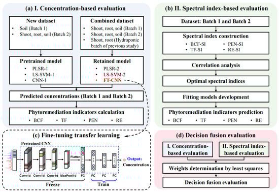
Figure 1.
Flowchart of data analysis process: (a) phytoremediation evaluation based on concentration prediction; (b) phytoremediation evaluation based on spectral index; (c) schematic of fine-tuning transfer learning; (d) integration of concentration-based and spectral index-based evaluation. Conv1d: convolutional layer; MaxPool1d: max pooling layer; FC: fully connected layer.
2.5.1. Concentration-Based Evaluation of Phytoremediation Effectiveness
The typical raw spectra collected by ME5000 and SR-500i are shown in Figure S1. According to the National Institute of Standards and Technology (NIST) database [37], characteristic spectral lines, such as Cd II 214.44 nm, Cd II 226.50 nm, Cd I 228.80 nm, Zn I 213.86 nm and some nutrient elements were observed. To enhance spectral stability and reduce fluctuations, outlier spectra from each pellet were removed using the median absolute deviation (MAD) method [38,39]. Specifically, spectra with intensity deviations exceeding 2.5 times the MAD were identified as outliers and removed to ensure data quality. The remaining spectra were averaged and area-normalized. Given that LIBS spectra contain numerous sources of noise and redundant information, feature extraction using competitive adaptive reweighted sampling (CARS) and CatBoost significantly reduced over 99% of features while preserving predictive power. Specifically, 365 and 450 features were selected for Cd and Zn analysis, respectively, from SR-500i and ME5000 spectrographs (Tables S1 and S2). The extracted CARS-CatBoost features, previously shown to yield strong performance for Cd and Zn quantification in both shoots and roots [28], were directly adopted for model development in this study.
Phytoremediation effectiveness was then evaluated by predicting Cd and Zn concentrations in shoots, roots, and soils, from which conventional indicators were derived (Figure 1a). Three models—partial least squares regression (PLSR), least squares-support vector machine (LS-SVM), and convolutional neural network (CNN)—had been pretrained on S. alfredii samples from hydroponic and soil cultivation experiments [28] (the soil cultivation experiment corresponds to Batch 1 in this study), and were referred to as PLSR-1, LS-SVM-1, and CNN-1. In this study, new data were introduced, including additional soil samples from Batch 1 and all plant and soil samples from Batch 2. To test model generalizability, the CARS-CatBoost features of these new samples were directly input into the pretrained models.
The detailed architecture of the CNN-1 models is provided in Table S3. The network consisted of three 1D-convolutional layers (64, 32, and 16 filters) followed by a 1D-max pooling layer (kernel size: 1 × 2, stride: 2) and three fully connected (FC) layers (128, 32, and 32 neurons). To prevent overfitting, Exponential linear unit (ELU) activation and batch normalization (BN) were applied. It is important to note that the input to the network was the reduced feature set (365 features for Cd and 450 for Zn) selected by CARS-CatBoost. Furthermore, for the FT-CNN (fine-tuning convolutional neural network) model, a transfer learning strategy was employed where the convolutional layers and the first FC layer were frozen, and only the last three layers (two FC layers and the output layer) were retrained. This strategy minimized the number of trainable parameters, ensuring that the available spectral dataset was sufficient to fine-tune the model effectively.
To further enhance the models’ performance on the new samples, datasets from both the new and old samples were combined for retraining. For PLSR and LS-SVM, this yielded totally new models (PLSR-2 and LS-SVM-2) that were retrained from scratch. In contrast, CNN supports transfer learning, which enables knowledge acquired from the source domain to be adapted to new data [40,41,42]. In this study, fine-tuning (FT) transfer learning was applied: all convolutional layers and the first fully connected layer of CNN-1 were frozen, and the last three fully connected layers were retrained to produce the FT-CNN models (Figure 1c). This strategy retained the general spectral representations while adapting to new data, improving generalization without training from scratch. It also improves generalization by incorporating incremental data updates, allowing the model to adapt to future sample variations effectively and make continuous improvements.
Model performance was evaluated using the coefficient of determination (R2), root mean square error (RMSE), and mean absolute percentage error (MAPE). Outlier inspection was also performed, where samples with residuals exceeding six standard deviations were excluded [43], resulting in the removal of two Zn-D soil samples (Batch 1) and one Zn-E soil sample (Batch 2).
2.5.2. Spectral Index-Based Evaluation of Phytoremediation Effectiveness
The second approach used spectral indices to directly and efficiently evaluate phytoremediation effectiveness (Figure 1b). Four spectral indices corresponding to traditional phytoremediation indicators were defined: bioconcentration factor-spectral index (BCF-SI), translocation factor-spectral index (TF-SI), plant effective number-spectral index (PEN-SI), and removal efficiency-spectral index (RE-SI). The equations are as follows:
where is the spectral intensity (peak) of the -th feature of shoot spectra, is the spectral intensity of the -th feature of root spectra, is the spectral intensity of the -th feature of soil spectra after remediation, is the spectral intensity of the -th feature of soil spectra before remediation, and is the dry weight of the shoot.
To identify optimal spectral indices, correlation analysis was conducted between constructed indices and traditional phytoremediation indicators (BCF, TF, PEN, and RE). The indices with the strongest correlations were selected, and their relationships with reference indicators were modeled using linear, polynomial, exponential, and power functions. The best-fitting models were then applied to predict phytoremediation indicators, enabling rapid evaluation of remediation effectiveness.
2.5.3. Accuracy Assessment of Spectra-Based Phytoremediation Evaluation
The recovery rate was adopted to assess the accuracy of spectral methods for evaluating phytoremediation effectiveness. It is calculated as:
where is the number of samples, is the predicted value of the phytoremediation indicator, and is the reference value of the phytoremediation indicator. The recovery rate reflects the agreement between predicted and reference values, with a range of 80–120% considered acceptable.
3. Results
3.1. Cd and Zn Concentrations and Phytoremediation Indicators
Cd and Zn accumulation in S. alfredii, and their removal from soils, as measured by ICP-OES, are shown in Figure 2. The accumulation generally increased with higher treatment levels. However, accumulation appeared to reach saturation in groups of high treatment levels (e.g., Zn-C and Zn-D groups in Batch 1, and Zn-E and Zn-F groups in Batch 2). As a hyperaccumulator, S. alfredii efficiently took up Cd and Zn through roots and translocated them to shoots, resulting in significantly higher accumulation in shoots than in roots in most groups. In this study, as shown in Figure 3, the plants in Batch 1 exhibited better growth than those in Batch 2, leading to higher Cd and Zn accumulation in plants and greater soil metal removal in Batch 1.
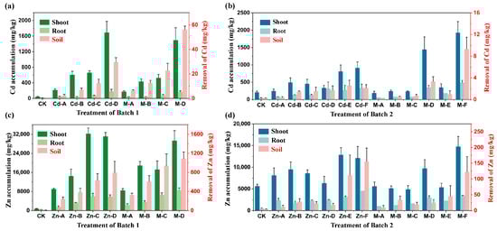
Figure 2.
Cd concentration in S. alfredii and removal from the soil of (a) Batch 1 and (b) Batch 2; Zn concentration in S. alfredii and removal from the soil of (c) Batch 1 and (d) Batch 2. The black y-axis titles correspond to the metal accumulation in shoots and roots, while the red y-axis titles correspond to the metal removal from the soil.
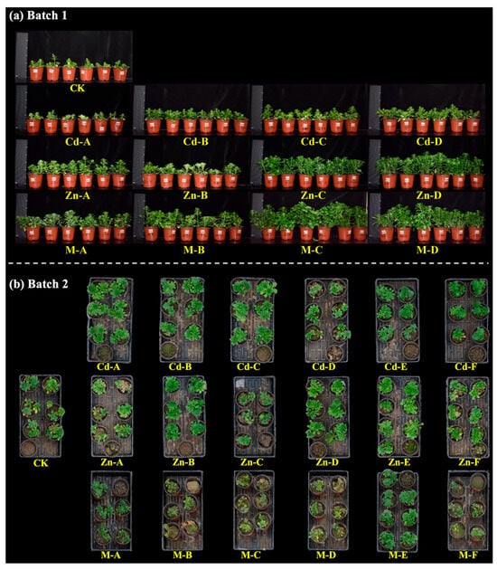
Figure 3.
Photos of S. alfredii of (a) Batch 1 and (b) Batch 2 at the harvest stage.
To evaluate the phytoremediation effectiveness of S. alfredii, BCF, TF, PEN, and RE were calculated and presented in Tables S4 and S5. In the Cd-only treatment groups, the BCF of Batch 2 was higher than that of Batch 1. However, because the overall growth status of the plants in Batch 2 was poorer, the biomass and TF were lower, limiting Cd translocation and resulting in a lower Cd removal from soil. Furthermore, the higher PEN of Batch 2 indicated that more plants were required to remove the same amount of Cd. For Zn-only treatment groups, Batch 1 outperformed Batch 2 across all indicators, indicating that S. alfredii in Batch 1 had a stronger ability to absorb, translocate, and accumulate Zn. Additionally, the plants in Batch 1 grew better and had higher biomass, leading to better remediation of soil Zn contamination. In the multi-metal treatment groups, BCF and TF for Batch 1 decreased compared to the individual treatments, likely due to competitive inhibition of metal uptake and accumulation in the presence of both metals. However, RE increased, possibly because the co-existence of both metals promoted plant growth, resulting in higher biomass and greater accumulation of metals. In Batch 2, the difference in phytoremediation effectiveness between the multi-metal and individual treatments was relatively small.
3.2. Evaluation of Phytoremediation Effectiveness Based on Concentration Prediction
3.2.1. Quantification of Cd and Zn in Shoots, Roots, and Soils
This study first developed quantitative models for Cd and Zn concentrations in shoots, roots, and soils. Model performance is summarized in Table 3 and Table 4. As described in Section 2.5.1, pretrained models (PLSR-1, LS-SVM-1, and CNN-1) were initially used to predict concentrations in new samples. However, they yielded extremely poor performance for direct prediction. As indicated by the dashes (“-”) in Table 3 and Table 4, these models resulted in negative R2test values when applied to the target domain (especially soils). These negative values indicate that the prediction error exceeded the inherent variance of the data, implying the models performed worse than a simple mean baseline. This failure is primarily attributed to severe matrix effects and domain shift, as the pretrained models were built using only S. alfredii samples and lacked soil information, making them unsuitable for direct prediction of complex soil matrices.
Table 3.
Prediction results for Cd quantification in S. alfredii and soil.
Table 4.
Prediction results for Zn quantification in S. alfredii and soil.
After retraining with the combined dataset of old and new samples, the prediction performance for the new samples improved significantly. LS-SVM-2 outperformed PLSR-2, with R2test values of 0.9729 and 0.7209 for Cd in plants and soils, respectively, and over 0.96 for Zn in both matrices. For all samples, LS-SVM-2 achieved R2test values of 0.9869 for Cd and 0.9994 for Zn, but with relatively high MAPE values (85.84% for Cd and 29.92% for Zn). The primary issue was the large prediction errors for soil samples, which significantly impacted the overall results. This may be attributed to the models’ poor prediction accuracy for low-concentration samples due to the sensitivity of MAPE to small values.
In contrast, the FT-CNN models achieved superior performance, as illustrated in regression scatter plots in Figure 4. In the range of 0–2467.70 mg/kg for Cd prediction (Figure 4a), the model yielded consistent R2test values for all samples, plant samples of Batch 2, and soil samples (0.9917, 0.9788, and 0.9824, respectively), with an overall MAPE of 13.62% for all samples. For Zn prediction (16.19–35,927.79 mg/kg) (Figure 4b), the FT-CNN model performed even better, with R2test values of 0.9956, 0.9733, and 0.9912 for all samples, plant samples of Batch 2, and soil samples, respectively, with MAPE below 10%. It should be noted that the high accuracies are largely attributed to the fact that the test samples, while physically independent, shared the same soil matrix characteristics as the training samples (derived from the same experimental batches). This demonstrates the model’s strong capability to adapt to specific soil environments through fine-tuning, but also implies that such high precision relies on the model having learned the specific matrix features. Therefore, expanding the diversity of soil samples remains necessary for broader applications.
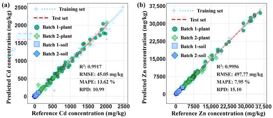
Figure 4.
Regression plots of FT-CNN models for (a) Cd and (b) Zn quantification in two batches of plants and soils. The light blue crosses represent the training set samples, and the dotted line represents the fitting line. The red dashed line represents the fitting line of the test set. The test set samples are distinguished by symbols: green circles for Batch 1 plants, light green crosses for Batch 2 plants, light blue squares for Batch 1 soil, and deep blue diamonds for Batch 2 soil. Note that the data points for soil samples are clustered near the origin due to their relatively low heavy metal concentrations compared to plant samples.
3.2.2. Phytoremediation Indicators Based on Concentration Prediction
Based on FT-CNN models, Cd and Zn concentrations in shoots, roots, and soils from both batches were predicted, and phytoremediation indicators were calculated and compared with reference indicators. The results for the Cd and Zn test sets are shown in Figure 5.
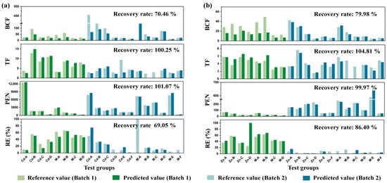
Figure 5.
Indicators to evaluate phytoremediation effectiveness (BCF, TF, PEN, and RE) based on concentrations in shoots, roots, and soils predicted by FT-CNN for (a) Cd and (b) Zn test set. Note: TF values for M-B and M-C groups in Batch 2 are missing due to insufficient biomass of their roots for pellet preparation.
The prediction accuracies for TF and PEN for both Cd and Zn datasets were high, with recovery rates close to 100%. This is likely because TF and PEN, being plant-based indicators, were less influenced by the matrix effects of LIBS spectra, resulting in more stable and accurate concentration predictions. Conversely, recovery rates for BCF and RE predictions were below 80%, indicating relatively poor accuracy, with predicted values generally underestimating reference indicators. In comparison, the prediction accuracies for Zn pollution remediation were better than for Cd. The recovery rate for RE prediction of the Zn dataset was greater than 80%, and the recovery rate for BCF was close to 80%, whereas, for the Cd dataset, both indicators had recovery rates below 80%. Recovery rates for BCF and RE were calculated separately for Batch 1 and Batch 2, revealing that the recovery rate of RE in Batch 2 was below 40%, indicating that concentration prediction errors of soil samples significantly affected the overall prediction performance of phytoremediation indicators.
3.3. Evaluation of Phytoremediation Effectiveness Based on Spectral Index
3.3.1. Spectral Index Construction
Different from the concentration-based approach, spectral indices were developed to establish a direct relationship with phytoremediation indicators, bypassing the intermediate concentration analysis step. This study proposed BCF-SI, TF-SI, PEN-SI, and RE-SI, calculated from the spectral intensities of the important features related to Cd and Zn.
Figure 6 shows the correlation heatmaps between spectral indices and reference indicators, where the vertical and horizontal axes represent the numerator and denominator of the spectral indices, and the color represents the strength of the Pearson correlation coefficient (r). For PEN-, ratio combinations corresponded to single spectral features, yielding 365 and 450 combinations for Cd and Zn, respectively, which was exactly the number of CARS-CatBoost features. For BCF-, TF-, and RE-, ratio combinations corresponded to two spectral features, yielding 133,225 (365 × 365) and 202,500 (450 × 450) combinations for Cd and Zn, respectively. From the correlation heatmaps, spectral indices with high correlations tended to appear together, as some spectral features closely related to target elements overlapped in wavelength, potentially introducing multicollinearity. Multicollinearity in the spectral indices might cause instability in the regression coefficients of multivariable models, reducing the model’s stability and generalizability. Therefore, selecting a few effective spectral indices was crucial for building stable models and practical applications.
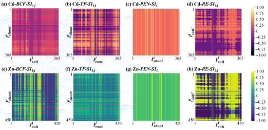
Figure 6.
Correlation heatmap between spectral indices (BCF-SI, TF-SI, PEN-SI, and RE-SI) and phytoremediation indicators (BCF, TF, PEN, and RE) for (a–d) Cd dataset and (e–h) Zn dataset.
Spectral indices with the highest correlation to reference indicators were selected, which were BCF-, TF-, PEN-, and RE- for Cd, and BCF-, TF-, PEN-, and RE- for Zn. The subscripts S and M following wavelengths represent SR-500i and ME5000, respectively. The relationships between these optimal spectral indices and reference indicators are shown in Figure 7. Among the selected spectral indices, the spectral feature wavelengths were close to or overlapped with the characteristic peaks of Cd and Zn according to the National Institute of Standards and Technology (NIST) database. For the Cd dataset, the spectral indices TF-, PEN- and RE- showed good correlations with TF, PEN, and RE, respectively (r > 0.7), while BCF- had a relatively weak correlation with BCF (r = 0.66). For the Zn dataset, the correlations of the spectral indices with reference indicators were higher than those for Cd, with all correlations exceeding 0.76. Among these, PEN- and RE- had very strong correlations with PEN and RE, respectively, with r over 0.9. For samples of both Batch 1 and Batch 2, the overall trends were consistent, with some overlap in the data distribution for TF and PEN indicators. The data distribution for RE showed a clear separation between samples of two batches, due to significant differences in the soil heavy metal removal effectiveness between the two batches of plants.
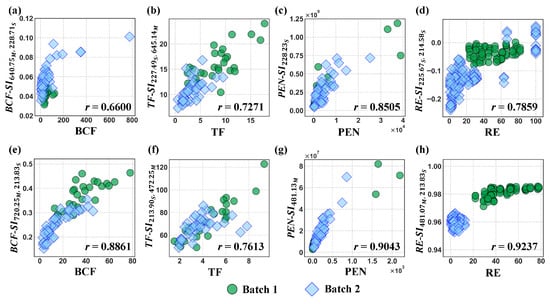
Figure 7.
Relationship between spectral indices with the highest correlation and phytoremediation indicators for (a–d) Cd dataset and (e–h) Zn dataset.
3.3.2. Phytoremediation Indicators Based on Spectral Index
The relationships between optimal spectral indices and reference indicators were modeled using linear, quadratic polynomial, exponential, and power functions. The best fit for each index was selected based on the highest R2 value. The effectiveness of the spectral index fitting was validated on the test set (Table 5).
Table 5.
Phytoremediation evaluation based on spectral index.
The results indicated that nonlinear functions (exponential, power, quadratic) generally provided the best fit between the spectral indices and the phytoremediation indicators. The R2 values of the fitting function models ranged from 0.5805 to 0.9084, suggesting that the model’s explanatory power varied significantly for different indicators. The prediction accuracy also varied. For Cd remediation, the recovery rates for the four indicators ranged from 107.45% to 145.16%, while for Zn, they ranged from 101.06% to 130.49%, suggesting a general tendency to overestimate values. In comparison, the evaluation of Zn remediation was more accurate than that of Cd, as the fitting function R2 values for BCF-SI, PEN-SI, and RE-SI were higher for Zn than for Cd, and except for PEN, the recovery rates for the indicators were closer to 100%, indicating better prediction accuracy.
For the evaluation of Cd remediation effectiveness, Cd-TF- provided a relatively good prediction for TF. Although it was not as accurate as the evaluation method based on concentration prediction, even when using only one index, the recovery rate was 107.45%, showing some potential for rapid evaluation of the translocation capacity of S. alfredii for Cd. The evaluation of Zn remediation was generally better than that of Cd. The fitting of Zn-RE- was the best (R2 = 0.9084), and the recovery rate for soil Zn removal prediction was higher than the evaluation method based on concentration prediction, with the recovery rate increasing from 86.40% to 101.06%. In addition, Zn-TF- showed good accuracy for TF prediction, with a recovery rate of 102.24%, outperforming the evaluation method based on concentration prediction. This suggests that spectral indices have great potential for predicting soil Zn removal efficiency and evaluating the Zn translocation capacity of S. alfredii, with the advantage of simpler calculations and easy operation, without the need to indirectly evaluate the phytoremediation effectiveness through heavy metal concentration predictions.
3.4. Evaluation of Phytoremediation Effectiveness by Integrating Concentration Prediction and Spectral Index
Decision fusion is a method that improves prediction performance by integrating the results of multiple methods or models. It leverages the strengths of each model to reduce the prediction error or uncertainty of a single model, thereby enhancing prediction accuracy and generalizability. To evaluate the phytoremediation effectiveness of S. alfredii, this study proposed two approaches: one is based on the Cd and Zn concentrations predicted by quantification models, and the other is based on direct evaluation using spectral indices. In this section, decision fusion was applied by combining the results of the two approaches. Specifically, for each of the BCF, TF, PEN, and RE indicators, the predicted values from both methods were used as common input features. The weights of these input features were determined using the training set through the least squares method, minimizing the error between the weighted combination results and the reference indicators to determine the optimal weights. In the test set, the optimal weights were applied to the predicted values from the two methods to generate the final prediction results.
The comparison of the phytoremediation evaluation results from the decision fusion with those from the individual methods is shown in Figure 8. Generally, the concentration-based evaluation method yielded lower recovery rates for the four indicators compared to the spectral index-based evaluation method. After decision fusion, the recovery rates for TF, PEN, and RE were between those of the two evaluation methods. Notably, the recovery rate of Cd RE prediction reached 100.01%, indicating that decision fusion significantly improved the evaluation accuracy and demonstrated its potential for rapid and accurate RE evaluation for Cd. The individual methods provided relatively good evaluation results for TF of Cd, and TF and PEN of Zn, and the evaluation results for these indicators remained stable after decision fusion. However, the prediction accuracy for BCF and Cd PEN showed a significant decline after decision fusion.
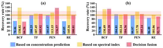
Figure 8.
Comparison of phytoremediation evaluation methods based on concentration prediction, spectral index, and decision fusion for (a) Cd dataset and (b) Zn dataset. The horizontal dotted line represents a recovery rate of 100%, and the pink shaded area represents the acceptable recovery range (80–100%).
In summary, this study introduced rapid evaluation methods for evaluating the phytoremediation effectiveness of S. alfredii based on transfer learning models, spectral index, and decision fusion, which provided good accuracy for evaluating TF, PEN, and RE. Additionally, the spectral-based phytoremediation evaluation method was also easy to operate, reducing the evaluation time per sample from over two hours using traditional methods to less than five minutes. This significant reduction in the evaluation time and period addressed the timeliness issues caused by traditional chemical analysis and held great potential for rapid phytoremediation evaluation.
4. Discussion
The study developed spectral methods for the evaluation of phytoremediation effectiveness based on concentration prediction and spectral index. This section highlights the advantages and limitations and discusses the potential efforts to enhance the field application of the methods.
4.1. Performance of Heavy Metals Quantification
Determining heavy metal concentrations in plants and soils and then calculating evaluation indicators are the most common approaches for assessing phytoremediation effectiveness. To enable rapid predictions of heavy metal concentrations using LIBS, accurate and stable models need to be developed. As discussed in previous studies, the matrix effect is a serious factor that impacts the quantitative accuracy of LIBS analysis. To mitigate these effects, CNN models based on CARS-CatBoost features were trained, which were applicable to shoots and roots of hydroponically and soil-cultivated S. alfredii for Cd and Zn quantification [28]. However, when evaluating phytoremediation effectiveness, soil plays a crucial role and is a matrix that differs significantly from plant tissue. Due to the influence of matrix effects, there have been few cases of joint modeling of soil and plants with large matrix differences. In this study, a new batch of S. alfredii (Batch 2) and two types of soil samples (fertilizer soil and rice paddy soil) were incorporated with previous samples. A fine-tuning transfer learning strategy was applied to avoid high computational costs while achieving excellent performance. The R2test values for Cd and Zn predictions exceeded 0.99, with MAPE values of 13.65% for Cd and 7.95% for Zn. With accurate heavy metal content predictions, the calculation of phytoremediation evaluation indices, such as BCF, TF, PEN, and RE, naturally became more reliable.
However, since the evaluation indicators are mostly ratios, errors in both components could be amplified. Additionally, as shown in Table 3 and Table 4, model performance for plant predictions was greater than for soil, which led to less accurate calculations for soil-related indicators like BCF and RE. It is worth noting that the soil types used in this study are representative of typical cultivation environments for S. alfredii phytoremediation, ensuring the method’s validity within this specific application scenario. However, given the significant matrix effects and spatial heterogeneity inherent in soils, relying on a limited number of soil types may restrict the direct generalizability of the model to completely unknown or vastly different geological fields. Therefore, future efforts should focus on two key aspects to extend the method to broader domains: first, increasing the diversity of soil types to build a more robust base model; and second, leveraging the proposed transfer learning framework to adapt the model to the specific environment of a new target site. This means that when applying the method to a new remediation project, a small set of local samples can be used to fine-tune the model, thereby ensuring accurate predictions despite the complex matrix variations encountered in real-world scenarios. Additionally, further spectral preprocessing methods for different matrices could be explored to reduce spectral differences. Advanced deep learning algorithms could also be investigated to enhance the accuracy of heavy metal quantification, which would improve the precision of phytoremediation effectiveness evaluation.
4.2. Strengths and Limitations of LIBS-Based Spectral Indices to Evaluate Phytoremediation Effectiveness
Constructing spectral indices to evaluate phytoremediation effectiveness offers a more direct approach. It only requires extracting one or two spectral features to calculate the corresponding indicators, using pre-established fitting functions. This method does not rely on detecting heavy metal concentrations and does not require the high computational cost or long inference time associated with machine learning or deep learning. Therefore, it is fast and efficient. It is also worth noting that while absolute spectral intensities are highly susceptible to matrix-induced fluctuations, the spectral indices constructed here utilize ratios of spectral features. This ratio-based structure functions as a form of self-normalization, which can effectively offset or balance out the matrix interferences to a certain extent, thereby enhancing the stability of the analysis in complex soil matrices. In the future, with the development of small, portable devices, this approach would be ideal for on-site applications, enabling high-throughput evaluation of phytoremediation effectiveness within minutes.
However, the spectral index-based evaluation method entails a trade-off between simplicity and robustness. The restriction to only two spectral features was intentionally designed to minimize computational load and facilitate future hardware miniaturization, thereby enabling the use of low-cost photodiodes with filters instead of full spectrometers. Nevertheless, unlike multivariate machine learning models that can utilize a large number of features to compensate for interference, this simplified input makes the spectral indices more dependent on the quality of the spectra and the effectiveness of the selected features. This is particularly challenging when dealing with matrices as different as soil and plants, where using only two spectral features can be easily influenced by matrix effects. External environmental factors and instrument noise can also increase errors in the results. Therefore, more advanced spectral preprocessing and feature extraction methods need to be explored to reduce spectral differences between different matrices and improve the representativeness of the selected features. Additionally, expanding the sample size and experimenting with various fitting function types could further enhance the model’s accuracy.
4.3. Future Perspectives
While the present study demonstrates the potential of LIBS combined with transfer learning and spectral indices for evaluating phytoremediation effectiveness, several avenues remain for future research to enhance applicability and generalization. First, expanding the diversity and number of samples—including multiple plant species, soil types, and heavy metal pollutants—will strengthen model robustness and enable broader environmental relevance. Field-based validation is also essential, including real-time and in situ measurements, to assess performance under natural variability and operational conditions. This could be facilitated by adapting the approach to handheld or portable LIBS devices, bridging laboratory findings with practical deployment scenarios. In addition, future methodological developments may focus on integrating phytoremediation evaluation with soil remediation management, providing actionable insights for sustainable remediation practices. From a data processing perspective, exploring end-to-end multimodal attention models that jointly learn from spectral, imaging, and soil metadata offers promise to improve predictive accuracy and generalization.
In the context of current evaluation methods that rely on heavy metal content detection, these approaches represent a significant step toward rapid on-site assessment of phytoremediation. With the potential efforts mentioned above, the speed and accuracy of spectral evaluation for phytoremediation effectiveness can be further improved, facilitating the application of these methods in the field.
5. Conclusions
This study established a LIBS-based system to rapidly and accurately evaluate the phytoremediation effectiveness of Cd/Zn co-hyperaccumulator S. alfredii. The main conclusions are as follows: (1) The previously developed CNN models for Cd and Zn quantification in shoots and roots of S. alfredii were fine-tuned to enable simultaneous detection in various matrices (shoots, roots, fertilizer soil, and rice paddy soil). The detection ranges for Cd and Zn were 0–2467.70 mg/kg and 16.19–35,927.79 mg/kg, respectively, with R2test values for Cd and Zn exceeding 0.99, and MAPE values below 14%. Based on the predicted concentrations, phytoremediation indicators were calculated, with TF and PEN achieving excellent recovery rates close to 100%. (2) Spectral indices for evaluating phytoremediation effectiveness, including BCF-SI, TF-SI, PEN-SI, and RE-SI, were proposed and selected with the highest correlation with reference indicators. Zn-RE- achieved a recovery rate of 101.06% for RE prediction, and Zn-TF- achieved a recovery rate of 102.24% for TF prediction, thus enabling accurate predictions of Zn removal and translocation of S. alfredii. (3) The evaluation method based on the integration of concentration prediction and spectral index achieved a recovery rate of 100.01% for predicting Cd removal efficiency. The LIBS-based spectral methods significantly reduce the time for evaluating phytoremediation effectiveness, providing support for rapid and efficient monitoring and evaluation of phytoremediation.
Supplementary Materials
The following supporting information can be downloaded at https://www.mdpi.com/article/10.3390/chemosensors14020029/s1. Figure S1: Average LIBS spectra collected by SR-500i and ME5000 spectrographs; Table S1: Spectral features for Cd analysis extracted by CARS and CatBoost; Table S2: Spectral features for Zn analysis extracted by CARS and CatBoost; Table S3: Detailed architecture of the CNN-1 models for Cd and Zn quantification; Table S4: Heavy metal concentrations and phytoremediation indicators of Batch 1; Table S5: Heavy metal concentrations and phytoremediation indicators of Batch 2.
Author Contributions
Conceptualization, Y.L. and F.L.; data curation, Y.L.; formal analysis, Y.L.; funding acquisition, F.L. and Y.L.; investigation, Y.L. and Z.T.; methodology, Y.L., Z.T., X.G., T.L. and W.K.; project administration, F.L.; resources, X.G., T.L. and W.K.; software, Y.L. and Z.T.; supervision, F.L.; validation, Y.L., Z.T. and F.L.; visualization, Y.L.; writing—original draft, Y.L.; writing—review & editing, F.L. All authors have read and agreed to the published version of the manuscript.
Funding
This research was funded by the National Natural Science Foundation of China (32371986, 61975174) and Zhejiang Guangsha Vocational and Technical University of Construction (2025ZX105).
Institutional Review Board Statement
Not applicable.
Informed Consent Statement
Not applicable.
Data Availability Statement
The data presented in this study are available on request from the corresponding author. The data are not publicly available due to the ongoing nature of the research project and proprietary restrictions.
Conflicts of Interest
The authors declare no conflicts of interest.
Abbreviations
The following abbreviations are used in this manuscript:
| BCF | Bioconcentration factor |
| CARS | Competitive adaptive reweighted sampling |
| CNN | Convolutional neural network |
| FT | Fine-tuning |
| ICP-OES | Inductively coupled plasma optical emission spectrometry |
| LIBS | Laser-induced breakdown spectroscopy |
| LS-SVM | Least squares-support vector machine |
| MAPE | Mean absolute percentage error |
| NIST | National Institute of Standards and Technology |
| PEN | Plant effective number |
| PLSR | Partial least squares regression |
| R2 | Coefficient of determination |
| RE | Removal efficiency |
| RMSE | Root mean square error |
| SI | Spectral index |
| TF | Translocation factor |
References
- Wu, Y.; Li, X.; Yu, L.; Wang, T.; Wang, J.; Liu, T. Review of Soil Heavy Metal Pollution in China: Spatial Distribution, Primary Sources, and Remediation Alternatives. Resour. Conserv. Recycl. 2022, 181, 106261. [Google Scholar] [CrossRef]
- Cunningham, S.D.; Berti, W.R.; Huang, J.W. Phytoremediation of Contaminated Soils. Trends Biotechnol. 1995, 13, 393–397. [Google Scholar] [CrossRef]
- Ranđelović, D.; Jakovljević, K.; Zeremski, T.; Pošćić, F.; Baltrėnaitė-Gedienė, E.; Noulas, C.; Mašková, P.; Jurković, J.; Baragaño Coto, D.; Milićević, T.; et al. Phytoremediation Potential of Metallophytes in Europe: Progress, Enhancement Strategies, and Biomass Utilisation. J. Environ. Manag. 2025, 391, 126516. [Google Scholar] [CrossRef]
- Yang, X.; Long, X.; Ni, W.; Fu, C. Sedum alfredii H: A New Zn Hyperaccumulating Plant First Found in China. Chin. Sci. Bull. 2002, 47, 1634–1637. [Google Scholar] [CrossRef]
- Yang, X.; Long, X.; Ye, H.; He, Z.; Calvert, D.V.; Stoffella, P.J. Cadmium Tolerance and Hyperaccumulation in a New Zn-Hyperaccumulating Plant Species (Sedum alfredii Hance). Plant Soil 2004, 259, 181–189. [Google Scholar] [CrossRef]
- Zhang, C.; Zhong, H.; Mathieu, J.; Zhou, B.; Dai, J.; Motelica-Heino, M.; Lavelle, P. Growing Maize While Biological Remediating a Multiple Metal-Contaminated Soil: A Promising Solution with the Hyperaccumulator Plant Sedum alfredii and the Earthworm Amynthas morrisi. Plant Soil 2024, 503, 201–215. [Google Scholar] [CrossRef]
- Yang, W.; Dai, J.; Liu, Z.; Deng, X.; Yang, Y.; Zeng, Q. Film Mulching Alters Soil Properties and Increases Cd Uptake in Sedum alfredii Hance-Oil Crop Rotation Systems. Environ. Pollut. 2023, 318, 120948. [Google Scholar] [CrossRef] [PubMed]
- Zhang, Q.; Wang, L.; Xiao, Y.; Liu, Q.; Zhao, F.; Li, X.; Tang, L.; Liao, X. Migration and Transformation of Cd in Four Crop Rotation Systems and Their Potential for Remediation of Cd-Contaminated Farmland in Southern China. Sci. Total Environ. 2023, 885, 163893. [Google Scholar] [CrossRef] [PubMed]
- Zhang, J.; Cao, X.; Yao, Z.; Lin, Q.; Yan, B.; Cui, X.; He, Z.; Yang, X.; Wang, C.-H.; Chen, G. Phytoremediation of Cd-Contaminated Farmland Soil via Various Sedum alfredii-Oilseed Rape Cropping Systems: Efficiency Comparison and Cost-Benefit Analysis. J. Hazard. Mater. 2021, 419, 126489. [Google Scholar] [CrossRef]
- Buscaroli, A. An Overview of Indexes to Evaluate Terrestrial Plants for Phytoremediation Purposes (Review). Ecol. Indic. 2017, 82, 367–380. [Google Scholar] [CrossRef]
- Song, B.; Zeng, G.; Gong, J.; Liang, J.; Xu, P.; Liu, Z.; Zhang, Y.; Zhang, C.; Cheng, M.; Liu, Y.; et al. Evaluation Methods for Assessing Effectiveness of in Situ Remediation of Soil and Sediment Contaminated with Organic Pollutants and Heavy Metals. Environ. Int. 2017, 105, 43–55. [Google Scholar] [CrossRef]
- Sun, Y.; Zhou, Q.; Diao, C. Effects of Cadmium and Arsenic on Growth and Metal Accumulation of Cd-Hyperaccumulator Solanum nigrum L. Bioresour. Technol. 2008, 99, 1103–1110. [Google Scholar] [CrossRef]
- Neugschwandtner, R.W.; Tlustoš, P.; Komárek, M.; Száková, J. Phytoextraction of Pb and Cd from a Contaminated Agricultural Soil Using Different EDTA Application Regimes: Laboratory versus Field Scale Measures of Efficiency. Geoderma 2008, 144, 446–454. [Google Scholar] [CrossRef]
- Bedabati Chanu, L.; Gupta, A. Phytoremediation of Lead Using Ipomoea aquatica Forsk. in Hydroponic Solution. Chemosphere 2016, 156, 407–411. [Google Scholar] [CrossRef]
- Antoniadis, V.; Levizou, E.; Shaheen, S.M.; Ok, Y.S.; Sebastian, A.; Baum, C.; Prasad, M.N.V.; Wenzel, W.W.; Rinklebe, J. Trace Elements in the Soil-Plant Interface: Phytoavailability, Translocation, and Phytoremediation—A Review. Earth-Sci. Rev. 2017, 171, 621–645. [Google Scholar] [CrossRef]
- Eid, E.M.; Galal, T.M.; Sewelam, N.A.; Talha, N.I.; Abdallah, S.M. Phytoremediation of Heavy Metals by Four Aquatic Macrophytes and Their Potential Use as Contamination Indicators: A Comparative Assessment. Environ. Sci. Pollut. Res. 2020, 27, 12138–12151. [Google Scholar] [CrossRef]
- Kumar, A.; Tripti; Raj, D.; Maiti, S.K.; Maleva, M.; Borisova, G. Soil Pollution and Plant Efficiency Indices for Phytoremediation of Heavy Metal(Loid)s: Two-Decade Study (2002–2021). Metals 2022, 12, 1330. [Google Scholar] [CrossRef]
- Zhang, Y.; Zhang, T.; Li, H. Application of Laser-Induced Breakdown Spectroscopy (LIBS) in Environmental Monitoring. Spectrochim. Acta Part B At. Spectrosc. 2021, 181, 106218. [Google Scholar] [CrossRef]
- Jia, X.; O’Connor, D.; Shi, Z.; Hou, D. VIRS Based Detection in Combination with Machine Learning for Mapping Soil Pollution. Environ. Pollut. 2021, 268, 115845. [Google Scholar] [CrossRef]
- Singh, P.; Pani, A.; Mujumdar, A.S.; Shirkole, S.S. New Strategies on the Application of Artificial Intelligence in the Field of Phytoremediation. Int. J. Phytoremediat. 2023, 25, 505–523. [Google Scholar] [CrossRef]
- Rathod, P.H.; Rossiter, D.G.; Noomen, M.F.; van der Meer, F.D. Proximal Spectral Sensing to Monitor Phytoremediation of Metal-Contaminated Soils. Int. J. Phytoremediat. 2013, 15, 405–426. [Google Scholar] [CrossRef] [PubMed]
- Rathod, P.H.; Brackhage, C.; Van der Meer, F.D.; Müller, I.; Noomen, M.F.; Rossiter, D.G.; Dudel, G.E. Spectral Changes in the Leaves of Barley Plant Due to Phytoremediation of Metals—Results from a Pot Study. Eur. J. Remote Sens. 2015, 48, 283–302. [Google Scholar] [CrossRef]
- Rathod, P.H.; Brackhage, C.; Müller, I.; Van der Meer, F.D.; Noomen, M.F. Assessing Metal-Induced Changes in the Visible and near-Infrared Spectral Reflectance of Leaves: A Pot Study with Sunflower (Helianthus annuus L.). J. Indian Soc. Remote Sens. 2018, 46, 1925–1937. [Google Scholar] [CrossRef]
- Lu, Y.; Nie, L.; Guo, X.; Pan, T.; Chen, R.; Liu, X.; Li, X.; Li, T.; Liu, F. Rapid Assessment of Heavy Metal Accumulation Capability of Sedum alfredii Using Hyperspectral Imaging and Deep Learning. Ecotoxicol. Environ. Saf. 2024, 282, 116704. [Google Scholar] [CrossRef]
- Feng, X.; Chen, H.; Chen, Y.; Zhang, C.; Liu, X.; Weng, H.; Xiao, S.; Nie, P.; He, Y. Rapid Detection of Cadmium and Its Distribution in Miscanthus sacchariflorus Based on Visible and near-Infrared Hyperspectral Imaging. Sci. Total Environ. 2019, 659, 1021–1031. [Google Scholar] [CrossRef] [PubMed]
- Winefordner, J.D.; Gornushkin, I.B.; Correll, T.; Gibb, E.; Smith, B.W.; Omenetto, N. Comparing Several Atomic Spectrometric Methods to the Super Stars: Special Emphasis on Laser Induced Breakdown Spectrometry, LIBS, a Future Super Star. J. Anal. At. Spectrom. 2004, 19, 1061–1083. [Google Scholar] [CrossRef]
- Guo, L.; Zhang, D.; Sun, L.; Yao, S.; Zhang, L.; Wang, Z.; Wang, Q.; Ding, H.; Lu, Y.; Hou, Z.; et al. Development in the Application of Laser-Induced Breakdown Spectroscopy in Recent Years: A Review. Front. Phys. 2021, 16, 22500. [Google Scholar] [CrossRef]
- Lu, Y.; Tao, Z.; Nie, L.; Guo, X.; Pan, T.; Chen, R.; Li, T.; Kong, W.; Liu, F. Quantitative Elemental Mapping of Heavy Metals Translocation and Accumulation in Hyperaccumulator Plant Using Laser-Induced Breakdown Spectroscopy with Interpretable Deep Learning. Comput. Electron. Agric. 2025, 230, 109907. [Google Scholar] [CrossRef]
- Li, S.; Xu, L.; Jing, Y.; Yin, H.; Li, X.; Guan, X. High-Quality Vegetation Index Product Generation: A Review of NDVI Time Series Reconstruction Techniques. Int. J. Appl. Earth Obs. Geoinf. 2021, 105, 102640. [Google Scholar] [CrossRef]
- Tayade, R.; Yoon, J.; Lay, L.; Khan, A.L.; Yoon, Y.; Kim, Y. Utilization of Spectral Indices for High-Throughput Phenotyping. Plants 2022, 11, 1712. [Google Scholar] [CrossRef]
- Kubier, A.; Wilkin, R.T.; Pichler, T. Cadmium in Soils and Groundwater: A Review. Appl. Geochem. 2019, 108, 104388. [Google Scholar] [CrossRef]
- Kaur, H.; Garg, N. Zinc Toxicity in Plants: A Review. Planta 2021, 253, 1–28. [Google Scholar] [CrossRef]
- Natasha, N.; Shahid, M.; Bibi, I.; Iqbal, J.; Khalid, S.; Murtaza, B.; Bakhat, H.F.; Farooq, A.B.U.; Amjad, M.; Hammad, H.M.; et al. Zinc in Soil-Plant-Human System: A Data-Analysis Review. Sci. Total Environ. 2022, 808, 152024. [Google Scholar] [CrossRef]
- Li, T.; Di, Z.; Yang, X.; Sparks, D.L. Effects of Dissolved Organic Matter from the Rhizosphere of the Hyperaccumulator Sedum alfredii on Sorption of Zinc and Cadmium by Different Soils. J. Hazard. Mater. 2011, 192, 1616–1622. [Google Scholar] [CrossRef]
- Chen, Z.; Liu, Q.; Chen, S.; Zhang, S.; Wang, M.; Mujtaba Munir, M.A.; Feng, Y.; He, Z.; Yang, X. Roles of Exogenous Plant Growth Regulators on Phytoextraction of Cd/Pb/Zn by Sedum alfredii Hance in Contaminated Soils. Environ. Pollut. 2022, 293, 118510. [Google Scholar] [CrossRef]
- Peng, J.; Liu, F.; Shen, T.; Ye, L.; Kong, W.; Wang, W.; Liu, X.; He, Y. Comparative Study of the Detection of Chromium Content in Rice Leaves by 532 nm and 1064 nm Laser-Induced Breakdown Spectroscopy. Sensors 2018, 18, 621. [Google Scholar] [CrossRef]
- NIST Atomic Spectra Database. Available online: https://www.nist.gov/pml/atomic-spectra-database (accessed on 10 December 2025).
- Leys, C.; Ley, C.; Klein, O.; Bernard, P.; Licata, L. Detecting Outliers: Do Not Use Standard Deviation around the Mean, Use Absolute Deviation around the Median. J. Exp. Soc. Psychol. 2013, 49, 764–766. [Google Scholar] [CrossRef]
- Miller, J. Reaction Time Analysis with Outlier Exclusion: Bias Varies with Sample Size. Q. J. Exp. Psychol. A 1991, 43, 907–912. [Google Scholar] [CrossRef]
- Shin, H.C.; Gao, M.; Lu, L.; Xu, Z.; Yao, J.; Summers, R.M. Deep Convolutional Neural Networks for Computer-Aided Detection: CNN Architectures, Dataset Characteristics and Transfer Learning. IEEE Trans. Med. Imaging 2016, 35, 1285–1298. [Google Scholar] [CrossRef]
- Vrbančič, G.; Podgorelec, V. Transfer Learning with Adaptive Fine-Tuning. IEEE Access 2020, 8, 196197–196211. [Google Scholar] [CrossRef]
- Peng, L.; Wu, H.; Gao, M.; Yi, H.; Xiong, Q.; Yang, L.; Cheng, S. TLT: Recurrent Fine-Tuning Transfer Learning for Water Quality Long-Term Prediction. Water Res. 2022, 225, 119171. [Google Scholar] [CrossRef] [PubMed]
- Montgomery, D.C. Introduction to Statistical Quality Control, 8th ed.; John Wiley & Sons: Hoboken, NJ, USA, 2019. [Google Scholar]


Disclaimer/Publisher’s Note: The statements, opinions and data contained in all publications are solely those of the individual author(s) and contributor(s) and not of MDPI and/or the editor(s). MDPI and/or the editor(s) disclaim responsibility for any injury to people or property resulting from any ideas, methods, instructions or products referred to in the content. |
© 2026 by the authors. Licensee MDPI, Basel, Switzerland. This article is an open access article distributed under the terms and conditions of the Creative Commons Attribution (CC BY) license.